Sharif University of Technology
Scientia IranicaTransactions A: Civil Engineering http://scientiairanica.sharif.edu
Predicting shear wave velocity of soil using multiple
linear regression analysis and articial neural networks
O. Ataee
a, N. Hafezi Moghaddas
a;, Gh.R. Lashkaripour
a, and
M. Jabbari Nooghabi
ba. Department of Geology, Faculty of Science, Ferdowsi University of Mashhad, Mashhad, Iran. b. Department of Statistics, Faculty of Science, Ferdowsi University of Mashhad, Mashhad, Iran. Received 16 May 2016; received in revised form 11 October 2016; accepted 28 January 2017
KEYWORDS Shear wave velocity; SPT;
Depth; Fine-content; Articial neural network; Multiple linear regression; Mashhad.
Abstract.This paper investigates the correlation between shear wave velocity and some of the index parameters of soils, including Standard Penetration Test blow counts (SPT), Fine-Content (FC), soil moisture (W ), Liquid Limit (LL), and Depth (D). The study attempts to show the application of articial neural networks and multiple regression analysis to the prediction of the shear wave velocity (VS) value of soils. New prediction equations are
suggested to correlate VSwith the mentioned parameters based on a dataset collected from
Mashhad city in the north east of Iran. The results suggest that, in the case of ANN method use, highly accurate correlations in the estimation of VSare acquired. The predicted values
using ANN method are checked against the real values of VS to evaluate the performance
of this method. The minimum correlation coecient obtained in ANN method is higher than the maximum correlation coecient obtained from the MLR. In addition, the value of estimation error in the ANN method is much less than that in the MLR method, indicating the role of higher condence coecient of the ANN in estimating VS of soil.
© 2018 Sharif University of Technology. All rights reserved.
1. Introduction
Shear wave velocity (VS) is a fundamental parameter
in dening the dynamic properties of soils, evaluating dynamic site response, and characterizing dynamic site [1,2]. The prole of VS in the ground is
consid-ered as the most reliable predictor of site-dependent properties from a seismic action in stable sites [3]. VS
is measured often by in-situ methods in low strain levels; therefore, the measured VS can be employed to
determine the maximum shear modulus (Gmax) of soil
deposit in dierent depths [1]. Gmax is an essential
*. Corresponding author.
E-mail addresses: [email protected] (O. Ataee); [email protected] (N. Hafezi Moghaddas);
[email protected] (Gh.R. Lashkaripour); [email protected] (M. Jabbari Nooghabi). doi: 10.24200/sci.2017.4263
input parameter for analyzing the dynamic stability of slopes, dams, embankments, etc. [4].
Although it is preferable to determining VS
di-rectly through eld tests, conducting these tests is mostly not feasible due to economic considerations, lack of space in urban areas, lack of specialized per-sonnel, and high noise levels in all situations [4-8]. In the absence of in-situ dynamic tests data, it is common worldwide to calculate VS through reported empirical
relationships between VS and other geotechnical soil
properties such as SPT, CPT, dry density, etc. [4]. SPT is one of the most economical and commonly employed in-situ tests involving very strong relationships with many of geotechnical soil properties. Many studies have proposed statistical relationships between VS and
SPT blow counts [1,3-6,8-20].
Generally, the relationships between VS and SPT
show considerable dispersion, which is probably due to the dierent methods employed in measuring VS and
SPT N value, as well as the geotechnical and geological conditions specic to any area. Another reason for low accuracy of these relationships is the type of regression analysis employed [21]. Traditionally, statistical meth-ods, such as simple and multiple regression analyses, are used in geotechnical engineering to create predic-tive models. All of conventional regression methods have limitations. Besides, empirical methods are not applicable to complicated and non-linear problems [22]. Articial Neural Network (ANN) is an over-simplied simulation of human brain made up of simple processing units, called neurons. This system is able to learn and generalize experimental data, even when the data are noisy, incomplete with a non-linear na-ture [23,24]. Unlike the conventional statistical models, the main advantage of ANN is that it does not require any prior knowledge related to the kind of relationship between input and output data. ANNs are also able to function very well in situations with limited data accessibility [25].
In recent years, Articial Intelligent (AI) methods have been widely used for predicting purposes [26,27]. So far, neural networks have been used for estimating and predicting some of the geotechnical properties of soil such as estimation of soil compaction pa-rameters [28,29], compressive and shear strength of soils [22,30,31], prediction of soil permeability [29,32], prediction of CBR in ne-grained soils [33], prediction of compressibility indices of saturated clays [34-36], pile bearing capacity [37,38], prediction of soil settle-ment [39], soil liquefaction [40-43], and analysis of slope stability [44-46]. Researchers have also used neural network models to predict VS value in oil wells
[26,47-50]. In addition, ANNs have been used to estimate and predict VS values of soils using geotechnical soil
properties such as CPT [51-53].
The present study aims to develop an optimal model to predict VS of soils in Mashhad city based
on the parameters of SPT, depth, ne content, liquid limit, and percentage of soil moisture. In this study, a multilayer perceptron with feed-forward backpropaga-tion is used for modeling VS in soil. The best neural
network model is found and selected through analysis of dierent models' performances (with dierent hidden layers and neurons in each layer). The purpose of this study is to identify properties of soil that have a more ecient role in predicting VS of soil; it also attempts
to compare the capabilities of neural networks and multiple regression technique in predicting VS value
using the variables mentioned above. 2. Study area
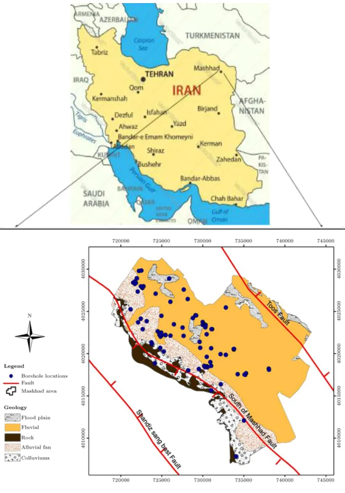
This study was carried out in Mashhad, Iran, which is the second most populated city in the center of Kho-rasan Razavi province in Iran. Mashhad is located at
36:10-36:24N latitude and 59:25-59:43E longitude
in the northeast of Iran. It is situated on Mashhad plain, which is covered with thick Quaternary alluvial sediments. Kashafrood River is the main drainage sys-tem of Mashhad plain as well as the streams originating from the southern parts of Mashhad (Figure 1).
From the seismotectonical perspective, Mashhad is situated between two folded-thrusted mountains (Koppe-Dagh in northeast and Binalood in south-west). According to Berberian et al. [54], there were intense earthquake activities in the area in the past centuries, especially in the 18th century. The existence of active faults within a short distance and on the two sides of Mashhad plain indicates that this area has a high potential for earthquake. Shandiz, Kashafrood, Toos, south of Mashhad, the north of Neishaboor, and Kheirabad faults are the main active faults in this area [55].
Mashhad city is an earthquake-prone area and is situated in the high-risk earthquake zone, with 0.30-0.35 g maximum acceleration in return period of 475 years, according to the Iranian Code of Practice for Seismic Resistance Design of Buildings (Standard No. 2800) [56]. These issues indicate the seismic vulnerability of Mashhad city; hence, an accurate estimation of VS for this city is required.
3. Materials and methods 3.1. Regression
Regression analysis is one of the analytical instruments widely applied to the investigation of relationships between a dependent variable and a set of independent (predictor) variables. Regression analysis is either linear or non-linear. In linear regression, data are mod-eled using linear-independent variables or predictive functions. In non-linear regression, data are modeled using a function that is a non-linear combination of model parameters. This type of regression is dependent on one or more independent variables. Regression analysis is one of the common methods for creating predictive models between VS and soil geotechnical
properties, including SPT and CPT. In addition to SPT, this paper aims to study the inuence of ne content, soil moisture, liquid limit, and soil depth on estimating VS value. Therefore, Multiple Linear
Regression analysis (MLR) will be employed. 3.2. Multiple Linear Regression analysis
(MLR)
Simple linear regression is a useful technique to predict a response based on a single predictor variable. How-ever, in practice, it often occurs that there is more than one predictor. MLR is used when there are more than one explanatory variable in a model, which can help explain or predict the response variable; therefore, all
of these explanatory variables are put into the model to carry out a multiple linear regression analysis. Then, the MLR equation is given as follows:
Y = 0+ 1X1+ 2X2+ + pXp+ "; (1)
where Xp represents the pth predictor, and p
quan-ties the relation between the variable and response. p is interpreted as the mean eect on Y of a
one-unit increase in Xp, holding all other predictors xed.
Regression coecients, 0; 1 p, in Eq. (1) are
unknown and must be estimated using the least squares approach as is the case in simple linear regression [57]. 3.3. Articial Neural Network (ANN)
ANN is a massively parallel-distributed information processing system with certain performance character-istics, simulating the biological neural networks of the human brain [58]. A neuron is the basic component of the neural networks that accepts and sums up inputs, applies a transfer function, which is normally nonlinear, and gives the result that is as either a model prediction or input into other neurons. An articial neural network is a combination of many such neurons connected in a systematic way. Neurons with the same properties in an ANN are ordered in groups, called layers [33]. One-layer neurons are connected to the neurons of the adjacent layers (not to the neurons of the same layer). The strength of connection between the two neurons in adjacent layers is recognized through the strength of connection or weight.
Usually, an ANN has three layers: one input layer, one hidden layer, and one output layer. Since ANNs have an error tolerance and the ability to work with incomplete data, they can easily produce models for complicated problems. In particular, for semi-structural or non-semi-structural problems, neural network models can provide very successful results. Further-more, they are faster and more reliable than the traditional methods are [23].
3.4. Multi-Layer Perceptron (MLP)
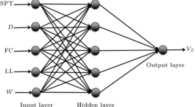
MLPs, also known as feed-forward neural networks, typically trained with back propagation algorithm, are usually used for prediction. Neurons in such networks are arranged in dierent layers (typically one input layer, one or more hidden layers, and one output layer) each of which is interconnected to its preceding and following layers. Figure 2 depicts a feed-forward three-layer ANN with the description of input and output layers employed in the current study. Connections between neurons have weights associated with them. These weights determine the strength of inuence that one neuron can have on another. From the input layer and through the processing layer(s), information ows to the output layer to generate predictions. During training, the network learns to generate predictions
Figure 2. Architecture of multilayer neural network for this study.
that are more accurate through adjusting the connec-tion weights so that predicconnec-tions can be matched with target values for specic records.
Determining the network architecture requires the optimum number of hidden layers between input and output layers and the optimum number of neurons in each hidden layer. That is one of the most important and most complicated parts of designing neural net-works, as there is no single theory or accepted rule for determining the optimal network architecture [59-61]. The number of hidden layers and their neurons is mostly determined by trial and error [62,63].
3.5. Data preparation and normalization The dataset used in this study was collected from geotechnical and geophysical reports from civil engi-neering projects done across Mashhad city by con-sulting engineering companies. Data related to 85 drilled boreholes were employed in data analysis. A complete dataset of six variables was required for this study; nally, 185 soil samples were used for regres-sion analysis, neural network design, and its accuracy evaluation. The model input variables selected for the present study are SPT, LL, W , FC, and D; the target or output variable is VS of the soil.
In most of the datasets, there is a lot of variability in the scale of range elds. Therefore, to nullify the eect of scale, range elds are transformed to have the same scale for all. In this situation, normalization can speed up the training process and improve the accuracy of the output model. Range elds are rescaled in Clementine to have values between 0 and 1. In this study, before inserting data into ANN, the input and output datasets were normalized through the following formula [64]:
xnormalized= xxactual xmin
max xmin ; (2)
where xnormalized is the normalized value of the
ob-served variable, xactualis the real value of the observed
variable, and xmax and xmin are the maximum and
respectively. When the function of the network is complete, network outputs are post-processed so that data can be converted into non-normalized units [28]. For ANN modeling, data are divided randomly into three categories of training, testing, and validation [60]. The network is trained by the rst category of data. The training set is also used for adjusting the weights of the connections. The validation set is used to test the performance of the network in dierent stages of training. When the training is successful, the testing set is used to evaluate the performance of the model.
The dataset collected from the Mashhad city region was rst analyzed for possible relationships between the parameters, and those variables which seemed likely to be inuential in predicting VS were
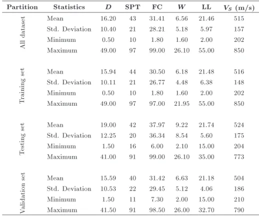
separated. Finally, ve main parameters, including SPT, LL, W , FC, and D, were considered as input parameters in MLR and ANN models. In designing a neural network, data were divided into training, testing, and validation sets. From 185 datasets used in this study, 80% (137 samples) were employed for training the model, 10% (19 samples) for testing the model, and 10% (29 samples) for validation of ANN analysis. All data were employed in regression analysis. Table 1 shows descriptive statistics related to the input and output parameters for all sets.
3.6. Performance evaluation criteria
For the assessment of methods, the obtained results
from each model (MLR and ANN) were evaluated based on dierent criteria. There are many criteria for assessing the performance of models. In this section, the eciency criteria used in this study are presented and evaluated. There are four criteria herein: the correlation coecient (R), coecient of determination (R2), Root Mean Square Error (RMSE), and Mean
Absolute Error (MAE). Each of the above criteria used in this study was computed through the following equations:
3.6.1. Pearson Correlation Coecient (R)
R can be used to estimate the correlation between model and observations:
R =
Pn
i=1(mi m) (p i p)
qPn
i=1(mi m) Pni=1(pi p)2
; (3)
where mi is the measured value, Pi is the predicted
value, m is the mean of measured values, and P is the mean of predicted values.
3.6.2. Coecient of determination or the square of the Pearson correlation coecient (R2)
R2describes how much of the variance between the two
variables is described by the linear t. 3.6.3. Root Mean Square Error (RMSE)
The RMSE of a model prediction is dened as the square root of the mean squared error:
Table 1. Descriptive statistics of input and output data.
Partition Statistics D SPT FC W LL VS (m/s)
All
dataset
Mean 16.20 43 31.41 6.56 21.46 515
Std. Deviation 10.40 21 28.21 5.18 5.97 157
Minimum 0.50 10 1.80 1.60 2.00 202
Maximum 49.00 97 99.00 26.10 55.00 850
T
raining
set Mean 15.94 44 30.50 6.18 21.48 516
Std. Deviation 10.11 21 26.77 4.48 6.38 148
Minimum 0.50 10 1.80 1.60 2.00 202
Maximum 49.00 97 97.00 21.95 55.00 850
T
esting
set Mean 19.00 42 37.97 9.22 21.74 524
Std. Deviation 12.25 20 36.34 8.54 5.60 175
Minimum 1.50 16 6.00 2.10 15.00 204
Maximum 41.00 91 99.00 26.10 35.00 773
V
alidation
set Mean 15.59 40 31.42 6.63 21.18 504
Std. Deviation 10.53 22 29.45 5.12 4.06 186
Minimum 1.50 11 7.30 2.00 15.00 210
RMSE = rPn
i=1(mi pi)2
n ; (4)
where n is the number of data presented in the database.
3.6.4. Mean Absolute Error (MAE)
The Mean Absolute Error (MAE) is a quantity used to measure how close predictions are to the eventual outcomes. The mean absolute error is given by:
MAE = Pn
i=1jmi pij
n : (5)
4. Results and discussion 4.1. Regression analysis
As previously mentioned, ve independent variables for multiple regression analysis were selected. At rst, the relationships between VS and each of the independent
variables were studied. The relationship between VS
and SPT as well as VS and depth has a power-law
form [1-20]. Therefore, the most preferred functional form of relation between SPT and VS proposed in
literature (VS = a Nb) has been used as the main
format for MLR analysis. This equation is given below: VS = a Nb Dc FCd We LLf: (6)
In this equation, N, D, FC, W , and LL represent SPT, depth, ne-content, moisture content, and liquid limit, respectively, and a to f are coecients that should be determined by regression. The power-law form of this model allows us to write it as follows:
log VS = log a + b log N + c log D + d log FC
+ e log W + f log LL: (7) In this case, the linear regression can be used to determine the constant values. MLR analysis was performed on 31 possible combinations of independent variables. After comparing the results, nine combina-tions whose coecient of determination exceeded 0.5 were selected to obtain the best model to govern VS.
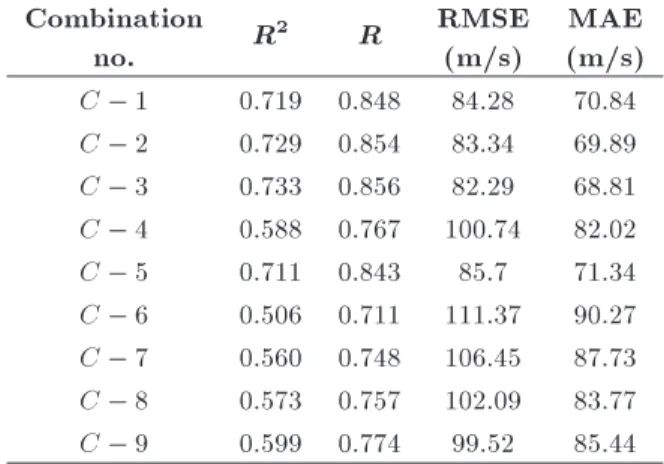
The combination of input variables in dierent models in this study is given in Table 2. The MLR regression analysis was performed using SPSS software, and the criteria for performance evaluation were calculated for each combination, as shown in Table 3.
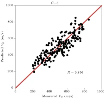
A comparison of the above results demonstrates that C 3 with a higher correlation coecient and coef-cient of determination (0.856 and 0.733, respectively) and smaller values of RMSE and MAE is the best model for predicting the value of VS of soil. It can be
observed that the combination of the three parameters, including D, SPT, and FC (silt and clay), shows the better correlation with VS. Figure 3 shows the scatter
plot of VS values predicted by MLR and its measured
values in the eld.
Table 2. Input and output for the dierent combinations. Combination
no. Input Output
C 1 D, SPT, LL
VS
C 2 D, SPT, W
C 3 D, SPT, FC
C 4 D, FC, W
C 5 D, SPT
C 6 D, LL
C 7 D, W
C 8 D, FC
C 9 SPT
Table 3. Performance evaluation criteria for the dierent combinations obtained by MLR analysis.
Combination
no. R2 R
RMSE (m/s)
MAE (m/s) C 1 0.719 0.848 84.28 70.84 C 2 0.729 0.854 83.34 69.89 C 3 0.733 0.856 82.29 68.81 C 4 0.588 0.767 100.74 82.02 C 5 0.711 0.843 85.7 71.34 C 6 0.506 0.711 111.37 90.27 C 7 0.560 0.748 106.45 87.73 C 8 0.573 0.757 102.09 83.77 C 9 0.599 0.774 99.52 85.44
4.2. Articial neural network development In this study, a FFBP-based ANN solver (Clementine data mining system) was used for designing and testing ANN models. Clementine is a preeminent data-mining toolkit widely used in academic researches and indus-trial applications. To apply Clementine ANN solver, like other FFBP-based software products, diverse net-work architectures should be examined to obtain the best result. The rst step in this process is to select input and output variables for this study, selected in prior sections.
In the next step, the number of hidden layers and neurons in each layer is dened for the model. There is no obvious solution for determining hidden layers and neurons for the ANN network. Although Zhang et al. [65] suggested that the optimum number of hidden layers in FFBP architecture is mostly one or two, some researchers have also suggested that, between n and 2n, hidden neuron is enough for FFBP models [66].
Generally, there are two fundamental approaches to constructing a FFBP network [67]. In a method called additive or constructive, the model starts with a minimal network consisting of a single hidden layer, and, gradually, hidden layers and neurons are added
Figure 3. Scatter plot of measured VS versus predicted
VS for the best model by MLR analysis.
and the eectiveness of the obtained model is evalu-ated using the evaluation instruments. In the second approach, the model starts with a very large network; moreover, pruning algorithm is used to reduce the size of the model [68].
Clementine provides both approaches: The dy-namic method uses the additive approach. In this state, the network topology changes during the training phase by the neurons that are added so that the network can obtain an optimum performance, while the system also monitors lack of improvement and overtraining. This process continues until no improvement can be achieved from the future model expansion. Conceptually, the prune method is dierent from the dynamic method. The prune method starts with a large network and, then, gradually prunes it by removing the unhelpful neurons from the input and hidden layers. There are two stages for pruning: pruning the hidden neurons and the input neurons. The two-stage process iterates continuously until the overall stopping criteria are met. These two stages are described below. The training process in this approach discards the weakest hidden neurons and selects the optimal size of the hidden layers. When one hidden layer is obviously enough, another option called Quick can be used where a simple mode creates a network with one hidden layer and at-tempts to determine the number of hidden neurons giv-ing the best results. The stoppgiv-ing rules in Clementine include a measure of desirable accuracy, the number of cycles on which the model is run, and the real amount of time in which the model is allowed to run.
In the present study, combinations of these ap-proaches were used to reach the best results. During the construction of these models, the prevent over-training parameter is always in the selection mode
to prevent the overtraining of the model. Input and output data were normalized before being inserted in the network. To design the neural network, the dataset was randomly divided into three discrete sets called training, testing, and validation (80%, 10%, and 10%, respectively). Only those data concerning the training set are used by neural network to learn the existing patterns in the data and optimize model parameters. During network training, the optimum numbers of neurons in the hidden layer and the learning rate are calculated. The training phase stops when the varia-tion of error becomes suciently small. After building a model using the training set, the performance of the trained model must be validated using new data. To get a more realistic estimation of how the model would perform with unseen data, we must allocate a part of the data not trained during the training process to this purpose. This set of data is known as the Validation Set. The testing set includes the unseen data for evaluating the performances of various candidate model structures and testing the network's generalization.
In this study, data analysis with neural networks was performed using the SPSS Clementine software. The ANN analysis was also carried out on nine selected combinations of independent variables in the previous sections. Dierent network methods were employed for each combination. In addition, the method was selected capable of estimating the value of the target parameter with higher accuracy and the least number of hidden layers and hidden neurons.
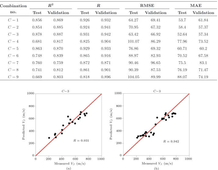
The performance criteria required for evaluating the accuracy of the designed models were computed for the training, testing, and validation stages (Table 4). Based on the model performance in validation stage, the best ANN model was determined. By comparing the evaluation criteria in Table 4, compared with other combinations, the combination (C 3) involving a structure of 3-2-3-1, which has the highest value of correlation and coecient of determination and the lowest values of RMSE and MAE, was selected as the optimal model in neural network analysis. With respect to this combination, it was observed that the values of RMSE and MAE were obtained as 63.42 and 52.64 m/s for testing set and as 66.92 and 57.34 m/s for validation set, respectively. Therefore, concerning certain ndings through regression analysis, it can be concluded that VS correlates well with SPT, FC, and
D. Results showed that high correlation coecient and low RMSE values were also obtained for C 2 and C 5 in both ANN and MLR methods, implying that the composition of two parameters SPT and depth of soil could be good estimators for predicting VS; however,
joining parameters, such as FC and W , would improve the prediction accuracy.
Furthermore, the coecient of determination for both of the testing and validation data shows that the
Table 4. Performance criteria for dierent models in testing and validation stage by ANN method. Combination
no.
R2 R RMSE MAE
Test Validation Test Validation Test Validation Test Validation
C 1 0.856 0.869 0.926 0.932 64.27 69.41 53.7 61.84
C 2 0.854 0.885 0.924 0.941 70.95 67.32 58.4 57.37
C 3 0.878 0.887 0.931 0.942 63.42 66.92 52.64 57.34
C 4 0.681 0.817 0.825 0.904 101.07 86.29 77.96 73.52
C 5 0.863 0.870 0.929 0.933 76.86 69.32 60.71 60.2
C 6 0.748 0.839 0.865 0.916 88.97 82.93 70.52 67.58
C 7 0.760 0.759 0.872 0.871 90.46 96.65 75.5 83.1
C 8 0.741 0.812 0.861 0.901 90.39 87.53 76.19 71.47
C 9 0.669 0.803 0.818 0.896 104.05 89.99 88.07 74.19
Figure 4. Relationship between measured and predicted shear wave velocity by ANN analysis in (a) testing and (b) validation phase.
predicted values of VS, using ANN method, show a
reasonably good correlation with actual values. Fig-ure 4 shows the relationship between the actual and predicted values of VS using the ANN in testing and
validation phases for the optimal model.
4.3. Comparison between ANN predictions and results of MLR
Combinations 1 to 9 were analyzed using both ANN and MLR methods. The predicted VS by the ANN
models for the testing and validation sets was compared with the estimated VS by multiple regression analysis
models. The MAE, RMSE, and R2 values extracted
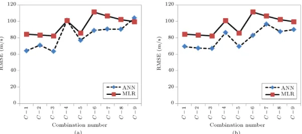
from ANN and MLR methods for dierent combina-tions are depicted in Figures 5, 6, and 7. Figures 5 and 6 show that the values of RMSE and MAE obtained from regression analysis are greater than the ANN method for all of the above combinations in both testing and validation sets. It is also obvious according to Figure 7 that the correlation coecient obtained
from ANN models is more than that from the MLR models, reecting the higher ability of ANN models for accurate prediction of VS value.
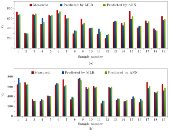
Finally, to compare the ANN and MLR methods and evaluate their performances, the predicted VS
values by these two methods for the optimal model (C 3) and for 20 random soil samples are presented in Figure 8. As the gure shows, the neural networks predict VS values closer to the actual (measured VS)
values for most of the samples. 5. Conclusions
The goal of this study is to evaluate the feed-forward neural networks as a possible tool for predicting VS
in Mashhad city. Five important input variables were used for predicting VS value. Dierent combinations of
these inputs have been studied. Nine combinations of these variables, which achieved the highest correlation coecient in regression analysis, were selected for
Figure 5. Comparison of RMSE values obtained by ANN and MLR: (a) Testing set and (b) validation set.
Figure 6. Comparison of MAE values obtained by ANN and MLR: (a) Testing set and (b) validation set.
Figure 7. Coecient of determination (R2) obtained by ANN and MLR: (a) Testing set and (b) validation set.
comparing the ANN and MLR methods. The neural networks were trained for nine mentioned combinations by the feed-forward backpropagation algorithm; it seems that it correlated the static properties of soil well with VS. To validate the neural network models, new
observation data were introduced to the networks and the forecasted VS were compared with actual values of
VS in the study area. Good agreement exists between
real and calculated data.
combina-Figure 8. Measured VS versus predicted VSby ANN and MLR methods for the best model (C 3): (a) Testing set and
(b) validation set.
tions of the three parameters including D, SPT N value, and FC give the best estimation of VS of soil.
The value of correlation coecient and coecient of determination obtained from the ANN method was higher than that of the MLR method. It should be mentioned that the error values computed through RMSE and MAE obtained from the MLR method were more than those extracted from the ANN method for all combinations under study. Therefore, it can be concluded that in comparison with MLR models, ANN models give more reliable prediction of VS. In other
words, ANN models have a better performance and can be used with a higher condence coecient to predict VS value of soil.
Acknowledgment
The authors appreciate cooperation from consulting engineering companies and soil mechanics laboratories in Mashhad city for providing their geotechnical re-porting for use in this paper. They also acknowledge the kind cooperation from the Zamin Physics Pooya Consulting Engineering Company for giving permission to use measured shear wave velocity.
Geolocation Information: Mashhad is the second most populated city in the center of the Khorasan Razavi province. It is located 850 km North East of Tehran, the capital of Iran, at 36:20north latitude and
59:35 east longitudes in the valley of the Kashafrood
River near Turkmenistan, between the two mountain ranges of Binalood and Hezar-Masjid, which are close to the borders of Afghanistan, and Turkmenistan. Role of funding sources: The work was not nan-cially supported by any funding sources.
References
1. Akin, M.K., Kramer, S.L., and Topal, T. \Empir-ical correlations of shear wave velocity (VS) and penetration resistance (SPT-N) for dierent soils in an earthquake-prone area (Erbaa-Turkey)", EngGeol., 119, pp. 1-17 (2011).
2. Fabbrocino, S., Lanzano, G., Forte, G., Santucci de Magistris, F., and Fabbroccini, G. \SPT blow count vs. shear wave velocity relationship in the structurally complex formations of the Molise Region (Italy)", Engineering Geology, 187, pp. 84-97 (2015).
3. Sil, A. and Sitharam, T.G. \Dynamic site character-ization and correlation of shear wave velocity with standard penetration test `N' values for the city of Agartala, Tripura state, India", Pure and Applied Geophysics, 171(8), pp. 1859-1876 (2014).
4. Chatterjee, K. and Choudhury, D. \Variations in shear wave velocity and soil site class in Kolkata city using regression and sensitivity analysis", Nat. Hazards, 69, pp. 2057-2082 (2013).
5. Hasancebi, N. and Ulusay, R. \Empirical correlations between shear wave velocity and penetration resistance for ground shaking assessments", Bulletin of Engineer-ing Geology and the Environment, 66, pp. 203-213 (2007).
6. Dikmen, U. \Statistical correlations of shear wave velocity and penetration resistance for soils", Journal of Geophysics and Engineering, 6, pp. 61-72 (2009). 7. Maheswari, R.U., Boominathan, A., and Dodagoudar,
G.R. \Use of surface waves in statistical correlations of shear wave velocity and penetration resistance of Chennai soils", Geotechnical and Geological Engineer-ing, 28, pp. 119-137 (2010).
8. Ghazi, A., Hafezi Moghadas, N., Sadeghi, H., Ghafoori, M., and Lashkaripour, G.L. \Empirical relationships of shear wave velocity, SPT-N value and vertical eective stress for dierent soils in Mashhad, Iran", Annals of Geophysics, 58(3), S0325 (2015). 9. Brandenberg, S.J., Bellana, N., and Shantz, T. \Shear
wave velocity as a statistical function of standard pen-etration test resistance and vertical eective stress at Caltrans bridge sites", Soil Dynamics and Earthquake Engineering, 30, pp. 1026-1035 (2010).
10. Shooshpasha, I., Mola-Abasi, H., Jamalian, A., Dik-men, U., and Salahi, M. \Validation and application of empirical shear wave velocity models based on standard penetration test", Computational Methods in Civil Engineering, 4(1), pp. 25-41 (2013).
11. Imai, T. \P- and S-wave velocities of the ground in Japan", In Proceedings of the IX, International Conference on Soil Mechanics and Foundation Engi-neering, pp. 127-132 (1977).
12. Imai, T. and Yoshimura, Y. \Elastic wave velocity and soil properties in soft soil (in Japanese)", Tsuchito-Kiso., 18(1), pp. 17-22 (1970).
13. Jafari, M.K., Shaee, A., and Razmkhah, A. \Dynamic properties of ne grained soils in south of Tehran", Soil Dynamics and Earthquake Engineering, 4, pp. 25-35 (2002).
14. Kiku, H., Yoshida, N., Yasuda, S., Irisawa, T., Nakazawa. H., Shimizu. Y., Ansal, A., and Erkan, A. \In situ penetration tests and soil proling in Ada-pazari, Turkey", In Proceedings of the ICSMGE/TC4 Satellite Conference on Lessons Learned from Recent Strong Earthquakes, pp. 259-265 (2001).
15. Lee, SHH. \Regression models of shear wave veloci-ties", Journal of the Chinese Institute of Engineers, 13, pp. 519-532 (1990).
16. Ohsaki, Y. and Iwasaki, R. \On dynamic shear moduli and Poisson's ratio of soil deposits", Soils and Foun-dations, 13(4), pp. 61-73 (1973).
17. Ohta, Y. and Goto, N. \Empirical shear wave velocity equations in terms of characteristics soil indexes", Earthquake Engineering and Structural Dynamics, 6, pp. 167-187 (1978).
18. Pitilakis, K.D., Anastasiadis, A., and Raptakis, D. \Field and laboratory determination of dynamic prop-erties of natural soil deposits", In Proceedings of the 10th World Conference on Earthquake Engineering, Rotherdam, pp. 1275-1280 (1992).
19. Seed, H.B. and Idriss, I.M. \Evaluation of liquefaction potential sand deposits based on observation of per-formance in previous earthquakes", Preprint 81-544, In Situ Testing to Evaluate Liquefaction Susceptibil-ity, ASCE National Convention, Missouri, pp. 81-544 (1981).
20. Sykora, D.E. and Stokoe, K.H. \Correlations of in-situ measurements in sands of shear wave velocity", Soil Dynamics and Earthquake Engineering, 20, pp. 125-136 (1983).
21. Dehghan Nayeri, G., Dehghan Nayeri, D., and Barkhordari, K. \A new statistical correlation between shear wave velocity and penetration resistance of soils using genetic programming", Electronic Journal of Geotechnical Engineering, 18, pp. 2071-2078 (2013). 22. Sivrikaya, O. \Comparison of articial neural networks
models with correlative works on undrained shear strength", Eurasian Soil Science, 42(13), pp. 1487-1496, Pleiades Publishing, Ltd (2009).
23. Dehghan, S., Sattari, Gh., Chehreh chelghani, S., and Aliabadi, M.A. \Prediction of uniaxial compressive strength and modulus of elasticity for Travertine sam-ples using regression and articial neural networks", Mining Science and Technology, 20, pp. 0041-0046 (2010).
24. Sarmadian, F. and Keshavarzi, A. \Developing pedo-transfer functions for estimating some soil properties using articial neural network and multivariate regres-sion approaches", International Journal of Environ-mental and Earth Sciences, 1(1), pp. 31-37 (2010). 25. Schaap, M.G., Leij, F.J., and Van Genuchten, M.Th.
\Neural network analysis for hierarchical prediction of soil hydraulic properties", Soil Science Society of America Journal, 62, pp. 847-855 (1998).
26. Maleki, S., Moradzadeh, A., Ghavami Riabi, R., Gholami, R., and Sadeghzadeh, F. \Prediction of shear wave velocity using empirical correlations and articial intelligence methods", NRIAG Journal of Astronomy and Geophysics, 3, pp. 70-81 (2014).
27. Mohammadi, H. and Rahmannejad, R. \The estima-tion of rock mass deformaestima-tion modulus using regres-sion and articial neural network analysis", Arabian Journal for Science and Engineering, 35(1A), pp. 67-77 (2009).
28. Gunaydm, O. \Estimation of soil compaction param-eters by using statistical analyses and articial neural networks", Environ. Geol., 57, pp. 203-215 (2009). 29. Sudha Rani, Ch. \Articial neural networks (ANNs)
for prediction of engineering properties of soils", Inter-national Journal of Innovative Technology and Explor-ing EngineerExplor-ing (IJITEE), 3(1), pp. 123-130 (2013).
30. Khanlari, G.R., Heidari, M., Momeni, A.A., and Abdilor, Y. \Prediction of shear strength parameters of soils using articial neural networks and multivariate regression methods", Engineering Geology, 131-132, pp. 11-18 (2012).
31. Mola-Abasi, H. and Shooshpasha, I. \Prediction of zeolite-cement-sand unconned compressive strength using polynomial neural network", The European Physical Journal Plus, 131(4), pp. 1-12 (2016). 32. Park, H.I. \Development of neural network model to
estimate the permeability coecient of soils", Marine Geosources and Geotechnology, 29(4), pp. 267-278 (2011).
33. Harini, H.N. and Naagesh, S. \Predicting CBR of ne grained soils by articial neural network and multiple linear regression", International Journal of Civil Engineering and Technology (IJCIET), 5(2), pp. 119-126 (2014).
34. Moayed, R.Z., Kordnaeij, A., and Mola-Abasi, H. \Compressibility indices of saturated clays by group method of data handling and genetic algorithms", Neural Computing and Applications, pp. 1-14 (2016). 35. Mola-Abasi, H. and Shooshpasha, I. \Prediction of
compression index of saturated clays (Cc) using poly-nomial models", Scientia Iranica, 23(2), pp. 500-507 (2016).
36. Kordnaeij, A., Kalantary, F., Kordtabar, B., and Mola-Abasi, H. \Prediction of recompression index using GMDH-type neural network based on geotech-nical soil properties", Soils and Foundations, 55(6), pp. 1335-1345 (2015).
37. Das, S.K. and Basudhar, P.K. \Undrained lateral load capacity of piles in clay using articial neural network", Computers and Geotechnics, 33, pp. 454-459 (2006). 38. Teh, C.I., Wong, K.S., Goh, A.T.C., and Jaritngam,
S. \Prediction of pile capacity using neural networks", J. Computing in Civil Engineering, ASCE, 11(2), pp. 129-138 (1997).
39. Sivakugan, N., Eckersley, J.D., and Li, H. \Settlement predictions using neural networks", Australian Civil Engineering Transactions, CE40, pp. 49-52 (1998). 40. Mola-Abasi, H., Shooshpasha, I., and Amiri, I.
\Pre-diction of liquefaction induced lateral displacements using GMDH type neural networks", Global Journal of Scientic Researches, 2(1), pp. 21-26 (2014). 41. Goh, A.T.C. \Probabilistic neural network for
evaluat-ing seismic liquefaction potential", Canadian Geotech-nical Journal, 39, pp. 219-232 (2002).
42. Kim, Y.S. and Kim, B.K. \Use of articial neural networks in the prediction of liquefaction resistance of sands", Journal of Geotechnical and Geoenvironmental Engineering, 132(11), pp. 1502-1504 (2006).
43. Ural, D.N. and Saka, H. \Liquefaction assess-ment by neural networks", Electronic Journal of Geotechnical Engineering, 3, pp. 1-27 (1998). (http://www.ejge.com/ 1998/JourTOC3.htm)
44. Cho, S.E. \Probabilistic stability analyses of slopes using the ANN-based response surface", Computers and Geotechnics, 36, pp. 787-797 (2009).
45. Ferentinou, M.D. and Sakellariou, M.G. \Computa-tional intelligence tools for the prediction of slope performance", Computers and Geotechnics, 34(5), pp. 362-384 (2007).
46. Wong, F.S. \Time series forecasting using back-propagation neural networks", Neurocomputing, 2, pp. 147-259 (1991).
47. Eskandari, H., Rezaee, M.R., and Mohammadnia, M. \Application of multiple regression and articial neural network techniques to predict shear wave velocity from well log data for a carbonate reservoir, South-West Iran", Cseg Recorder, pp. 42-48 (2004).
48. Moatazedian, I., Rahimpour-Bonab, H., Kadkhodaie-Ilkhchi, A., and Rajoli, M.R. \Prediction of shear and compressional wave velocities from petrophysical data utilizing genetic algorithms technique: A case study in Hendijan and Abuzar elds located in Persian Gulf", Geopersia, 1, pp. 1-17 (2011).
49. Akhundi, H., Ghafoori, M., and Lashkaripour, G.R. \Prediction of shear wave velocity using articial neural network technique, multiple regression and petrophysical data: A case study in Asmari reservoir (SW Iran)", Open Journal of Geology, 4, pp. 303-313 (2014).
50. Rezaee, M.R., Kadkhodaie Ilkhchi, A., and Barabadi, A. \Prediction of shear wave velocity from petrophysi-cal data utilizing intelligent systems: An example from a sandstone reservoir of Carnarvon Basin, Australia", Journal of Petroleum Science and Engineering, 55, pp. 201-212 (2007).
51. Mola-Abasi, H., Dikmen, U., and Shooshpasha, I. \Prediction of shear-wave velocity from CPT data at Eskisehir (Turkey) using a polynomial model", Near Surface Geophysics, 13(2), pp. 155-167 (2015). 52. Mola-Abasi, H., Eslami, A., and Tabatabaie Shourijeh,
P. \Shear wave velocity by polynomial neural networks and genetic algorithms based on geotechnical soil prop-erties", Arabian Journal for Science and Engineering, 38(4), pp. 829-838 (2013).
53. Shooshpasha, I., Kordnaeij, A., Dikmen, U., Mo-laAbasi, H., and Amir, I. \Shear wave velocity by support vector machine based on geotechnical soil properties", Natural Hazards and Earth System Sci-ences Discussions, 2(4), pp. 2443-2461 (2014). 54. Berberian, M. and Ghoreshi, M., Seismic-Fault
Haz-ard and Project Engineering of Thermal Power Plant of Nishapur, Seismotectonical Survey, Ministry of Energy, Power Engineering Corporation (Moshanir), Tehran (1989) (in Persian).
55. Azadi, A., Javan-Doloei, G.H., Hafezi Moghadas, N., and Hessami-Azar, K. \Geological, geotechnical and geophysical characteristics of the Toos fault located north of Mashhad, north-eastern Iran ", Journal of the Earth and Space Physics, 35(4), pp. 17-34 (2010) (in Persian).
56. Building and Housing Research Center, Iranian Code of Practice for Seismic Resistant Design of Buildings, Standard No. 2800, 3rd Edn., Tehran, Iran (2007). 57. James, G., Witten, D., Hastie, T., and Tibshirani, R.,
An Introduction to Statistical Learning with Applica-tions in R, Springer, New York, Heidelberg Dordrecht, London (2013).
58. Haykin, S., Neural Networks: A Comprehensive Foun-dation, 2nd. Ed. Prentice-Hall, Upper Saddle River, New Jersey, pp. 26-32 (1999).
59. Shahin, M.A., Jaksa, M.B., and Maier, H.R. \Ar-ticial neural network applications in geotechnical engineering", Australian Geomechanics, 36(1), pp. 49-62 (2001).
60. Isik, F. and Ozden, G. \Estimating compaction pa-rameters of ne and coarse grained soils by means of articial neural networks", Environmental Earth Sciences, 69, pp. 2287-2297 (2013).
61. Kisi, O. \Stream ow forecasting using dierent arti-cial neural network algorithms", Journal of Hydrologic Engineering. ASCE, 12(5), pp. 532-539 (2007). 62. Kanungo, D.P., Arora, M.K., Sarkar, S., and Gupta,
R.P. \A comparative study of conventional, ANN black box, fuzzy and combined neural and fuzzy weighting procedures for landslide susceptibility zonation in Dar-jeeling Himalayas", Engineering Geology, 85, pp. 347-366 (2006).
63. Kartam, N., Flood, I., and Garrett, J.H. \Articial neural networks for civil engineers", Fundamentals and Applications, ASCE, New York (1997).
64. Kayadelen, C. \Estimation of eective stress param-eter of unsaturated soils by using articial neural networks", International Journal for Numerical and Analytical Methods in Geomechanics, 32(9), pp. 1087-1106 (2008).
65. Zhang, G., Patuwo, E.B., and Hu, M.Y. \Forecasting with articial neural network: The state of the art", International Journal of Forecasting, 14, pp. 35-62 (1998).
66. Wang, H.B., Xu, W.Y., and Xu, R.C. \Slope stability evaluation using back propagation neural networks", Engineering Geology, 80, pp. 302-315 (2005).
67. Rivals, I. and Personnaz, L. \Neural-network con-struction and selection in nonlinear modeling", IEEE Transaction on Neural Networks, 14(4), pp. 804-819 (2003).
68. Ghiassi, M. and Nangoy, S. \A dynamic articial neu-ral network model for forecasting nonlinear processes", Computers & Industrial Engineering, 57(1), pp. 287-297 (2009).
Biographies
Omolbanin Ataee is a PhD Student at the Depart-ment of Geology at Ferdowsi University of Mashhad, Iran. Her main areas of research interest are soil mechanics, geostatistics and environmental geology. Naser Hafezi Moghaddas is currently a Professor of Engineering Geology at Ferdowsi University of Mash-had. His research interests focus on the landslide, site eect and micro zonation of earthquake, slop stability. Gholam Reza Lashkaripour is a Professor of Engi-neering Geology at Ferdowsi University of Mashhad. He teaches courses such as environmental geology, hydrology, advanced engineering geology, rock mechan-ics, groundwater and geotechnical problems, geological hazards, site investigation, and soils improvement at graduate and postgraduate levels.
Mehdi Jabbari Nooghabi is an Assistant Professor at the Department of Statistics at Ferdowsi University of Mashhad. He taught dierent courses such as sta-tistical applications in management, stasta-tistical quality control, time series, research method and statistical consulting, statistics for managers, business mathemat-ics and statistmathemat-ics, statistical analysis, special topmathemat-ics, ad-vanced applied statistics, statistics meteorology, linear models and their application in genetic improvement of farm animals, advanced methods of statistical in-ference, industrial statistics, and multivariate discrete and continuous analysis at graduate and postgraduate levels.