Vol.9 (2019) No. 6
ISSN: 2088-5334
Radial Basis Function (RBF) Neural Network: Effect of Hidden
Neuron Number, Training Data Size, and Input Variables on Rainfall
Intensity Forecasting
Soo See Chai
#1, Wei Keat Wong
#2, Kok Luong Goh
*, Hui Hui Wang
#3, Yin Chai Wang
#4 #Department of Software Engineering and Computing, Faculty of Computer Science and Information Technology, University Malaysia Sarawak (UNIMAS), Malaysia
E-mail:[email protected];[email protected];[email protected];[email protected] *
School of Innovative Technology, International College of Advanced Technology Sarawak (i-CATS), Malaysia E-mail: [email protected]
Abstract— Mean daily rainfall of more than 30mm could result in flood hazard. Accurate prediction of rainfall intensity could help in
forecasting of flash flood and help to save lives and properties. One of the common machine learning techniques in rainfall prediction is Radial Basis Function (RBF) neural network. Rainfall intensity is classified into four categories, i.e. light (<10mm), medium (11-30mm), heavy (31-50mm) and very heavy (>50mm) in this study. The rainfall intensity categories is forecasted using the RBF network model utilizing the daily meteorology data for Kuching, Sarawak, Malaysia. The input vectors being considered for the RBF network model are minimum, maximum and mean temperature (°C), mean relative humidity (%), mean wind speed (m/s), mean sea level pressure (hPa) and mean precipitation (mm) for the year 2009 to 2013. The prime focus in this paper is to analyse the ramification of the training data size, number of hidden neurons, and different input variables (i.e. combination of meteorology data) in influencing the performance of the RBF network model. From this study, it could be concluded that, the factor that would influence the performance of the RBF model is only the input variables used, if and only if the network model is equipped with sufficient number of hidden neurons and trained with adequate number of training data. Another interesting observation from this study is that, the RBF network model produced consistent result throughout the testing using a specific hidden neuron number when the RBF network is retrained and tested.
Keywords— rainfall; radial basis function; intensity; forecasting; meteorology data.
I. INTRODUCTION
Rainfall intensity refers to the measure of the amount of rain that falls over time and this data has been defined as the most critical flood hazard parameter [1-4]. Flood is one of the Earth’s most common and destructive natural disasters which accounts for the most significant death and financial lost [5]. Therefore, accurate prediction of rainfall intensity could help in lives and properties saving, as well as securing the national economic activities [6].
Rainfall forecasting could be done using the Numerical Weather Prediction (NWP) model, statistical methods and machine learning techniques [6]. By using the numerical solutions of atmospheric hydro thermodynamic equations, NWP, which is also known as physical models, high accuracy could be obtained as long as the complex and meticulous simulation of the physical equations in the atmosphere model is appropriately solved [7, 8]. However, this could sometimes lead to unsatisfactory due to the
In our previous work [16], the accuracy of the Backpropagation and Radial Basis Function (RBF) models for rainfall intensity categorization problem was compared. It became apparent that, RBF model, contrasting to Backpropagation neural network model, managed to maintain a consistent result while in terms of accuracy, Backpropagation neural network model is superior. In this research work, impact of different number of hidden neurons and training data, as well as the varied combination of input variables on the RBF model for categorization of the rainfall intensity using meteorology data of Kuching, Sarawak, Malaysia will be analyzed.
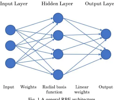
In 1988 [17], Broomhead and Lowe introduced the Radial Basis Function (RBF) network model. The overall architecture of a RBF model, as shown in Fig. 1, included three layers, namely, Input, Hidden and Output layers. There is only one single hidden layer in RBF neural network. This is different from a neural network that could possess multiple intermediary layers [18]. The outside information flowed into the network via the input layer. Using nonlinear transformation in the hidden layer, the information from outside is then processed. The output layer combined linear and non-linear radial basis functions [19]. There is an activation function in each hidden neuron. The Gaussian function has been commonly used in the hidden neuron as the activation function. Therefore, RBF model has a non-linear structure from input to the hidden layer, while the linear structure appears from the hidden layer to the output layer. The quantity of the hidden neurons in the hidden layer determines the complexity and generalization capability of the RBF model [18]. A RBF model is a preferred choice as it could be trained rapidly. Besides, its general applicability is also an important characteristic that makes this a common choice of artificial intelligent model [20].
Fig. 1 A general RBF architecture
RBF model was applied to forecast yearly rainfall and the two highest monsoon rainfall months (January and December) for Alexandria City, Egypt [21]. In their research work, a RBF model of single input and single output was constructed. Root Mean Square Error (RMSE) and correlation of coefficient (R2) were calculated as accuracy measures. It was shown that the RBF model managed to achieve RMSE of 27.13 with R2 = 0.94 for yearly rainfall prediction. For January and December, the RMSE values achieved were 10.61 and 10.85 respectively. The R2
achieves was 0.89 for January and 0.98 for December. Using single input and single output RBF neural network model, annual rainfall prediction for three areas in India showed that the RBF neural network model produced different accuracies [22]. The RMSE values achieved ranged from 25.6mm, 63.0mm to 66.4mm for these three areas with a coefficient correlation (R2) of more than 0.9.
As rainfall depends on many weather parameters, i.e. pressure, temperature, wind speed, etc., features selection should be considered in rain predicting algorithms. In [23], a feature selection algorithm for rainfall prediction was proposed and the accuracy of the multi-layer feed-forward neural network, RBF neural network, focused time-delay neural network, and nonlinear autoregressive exogenous input neural network was evaluated. Feature selection is done by sensitivity analysis of the input attributes by removing the non-effective weather attributes. It was noticed that all the evaluated neural network models performed better after the feature selection process.
II. MATERIALS AND METHOD
Sarawak, a state in East Malaysia, has an equatorial climate, which is symbolized by hot temperatures with high humidity [24]. The study area selected is the capital city of Sarawak, i.e., Kuching. Kuching city is situated at latitude and longitude coordinates of 1.5447 and 110.3652 and covers an area of 431 km2. The daily historical meteorology parameters, i.e. minimum, maximum and mean temperature (°C), mean relative humidity (%), mean wind speed (m/s), mean sea level pressure (hPa) and mean precipitation (mm) for the year 2009 to 2013 were collected from Malaysian Meteorological Department.
A. Data Pre-processing
Weather data is prone to miss values and the missing values would affect the performance of the underlying neural network model [25]. Therefore, before developing the network model, missing values were deleted from the data set.
B. Data Normalization
After cleaning the data, the data will next go through the normalization process. During data normalization, the data were scaled to -1 and +1. With this process, the capability of the network model developed in handling the data is increased. The calculation of the network model would be done faster and the network model developed will be able to obtain a good result [23]. In this research work, the input data was normalized using the formula below:
(1)
where:
:
output of the normalization:
maximum normalized value required:
minimum normalized value required:
data to be normalized:
maximum of input dataC. Different Categories of Rainfall Intensity
Four categories were used to categorize the rainfall intensity data collected in the year 2009 to 2013, i.e. light, moderate, heavy and very heavy rainfall using the intensity range shown in Table I [16].
TABLEI
RAINFALL INTENSITY CLASSIFICATION [25]
Rainfall Intensity Category Intensity range (mm)
Light <10
Moderate 11-30
Heavy 31-50
Very Heavy >50
D. RBF Neural Network Setup Properties
RBF model of a single hidden layer is termed a universal approximator as it can be used to approximate any function [26]. Research has also shown that RBF model is optimal when there are many training vectors. The setup properties of the RBF model are shown in TABLE II. The RBF model was trained with the starting of 10 hidden neurons as this number is larger than the total number of input parameters available. An increment of 50 hidden neurons is used for the other two network models tested in this section.
TABLEII
RBFNEURAL NETWORK SETUP PROPERTIES
Layers: 3 layers (input, hidden and output)
Learning Algorithm: Gaussian
Number of hidden neurons: 10, 50 and 100
E. Input and Output Data of RBF Neural Network
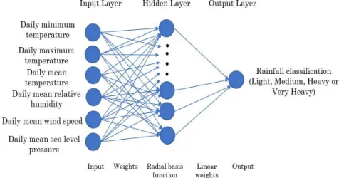
The six-meteorology data, i.e. minimum, maximum and mean temperature (°C), mean relative humidity (%), mean wind speed (m/s), mean sea level pressure (hPa) and mean precipitation (mm) are used as the input vector for the RBF model. An array of one of these meteorology data will serve as the input nodes of the RBF model. The rainfall classification, which is either light, moderate, bulky or very heavy will serve as the output of the model. The overall architecture of the RBF model used in this research work is illustrated in Fig. 2.
Fig. 2 The overall RBF architecture used in this research work.
F. Training and Testing Data
The RBF model learns via the examples given. This process serves as the training of the model. The trained network model is next tested using a set of sensed data. The
total of 60 months data obtained from 1st January 2009 to 31st December 2013 was grouped into five groups as shown in Table III. The testing data used was the one-month data from 1st December to 31st December 2013.
TABLE III
DIVISION OF TRAINING AND TESTING
G. Experiment Setup
To investigate the impact of different numbers of hidden neurons, training size and input variables on the accuracy of the rainfall intensity forecasting using RBF model, the following experiments are conducted.
1) The number of Hidden Neurons: The hidden layer,
together with the number of neurons in this layer, will influence the accuracy of the neural network model [27]. As RBF model is a single-weight network, the only influencing factor, in this case, will be the number of hidden neurons. Therefore, the testing of the number of hidden layers is excluded. For this section of the experiment, 59 months of data (1st January 2009 to 30th November 2013) will be used for training and the 1-month data from 1st December 2013 to 31st December 2013 will be used for testing (Group 5 in TABLE III). The number of hidden neurons tested was started with a minimum of 10 and in the increment of 50. Three network models of 10, 50 and 100 hidden neurons were developed. Each of these network models was trained and tested 15 times. This set of experiments is run prior to the following two other parts of experiments. At the end of the experiment in this section, the optimal hidden neurons will be obtained and used for the following two parts of experiments.
2) Training Data Size: It is well accepted that a small
training data set is not capable to train the network model appropriately [28]. With an increased number of training data, the generalization of the problem underlying would be better modeled by the neural network [16]. However, the performance of the model will converge at one point even with more training data provided [29]. As more training data does not help in increasing the network model performance, the use of more training data will be a waste of resources as well as adding complexity to the network model. Therefore, it would be beneficial to investigate the number of data that is minimal in order to train the RBF model to forecast the rainfall intensity accurately. To investigate these properties, the RBF model with the predetermined hidden neuron obtained from the experiment mentioned above will be used. The division of the training and testing data as shown in Table III is used for the research on the number of training data.
Training Data Size Test Data Size Group
12 months (1/1/2009 – 31/12/2019)
1 month (1/12/2013 – 31/12/2013)
1
24 months (1/1/2009 – 31/12/2010)
1 month (1/12/2013 – 31/12/2013)
2
36 months (1/1/2009 – 31/12/2011)
1 month (1/12/2013 – 31/12/2013)
3
48 months (1/1/2009 – 31/12/2012)
1 month (1/12/2013 – 31/12/2013)
4
59 months (1/1/2009 – 30/11/2013)
1 month (1/12/2013 – 31/12/2013)
3) Different Combination of Input Variables: The
objective of selecting the correct combination of meteorology data as the input variables is to identify the right predictor variables [30]. The use of the correct predictor variables would reduce the time in training the neural network model. Moreover, the correct predictor variables used will also increase the accuracy of the network performance as well as reducing the complexity of the network model. In this part of the experiment, the network model of m:x:1 will be used, where m is the number of different combinations of meteorology data, and x is the number of optimum hidden neurons obtained from the previous experiment. The output layer will only be one of the four rainfall intensity categories (refer to Table 1). A set of 15 different combinations of meteorology data as shown in Table IV are used in order to verify the optimum input for the RBF model.
TABLE IV
COMBINATION OF DIFFERENT METEOROLOGY DATA USED FOR
FEATURE SELECTION
III.RESULTS AND DISCUSSION
In this study, the Mean Square Error (MSE) and correlation coefficient (R2) are used as the evaluation units to measure the performance of the RBF model. The MSE
measures the average difference (errors) between the forecasted results and actual results. Lower MSE would mean better forecasted results obtained by the network model, i.e., the forecasted results obtained by the RBF model is closer to the actual results. On the other hand, R2 measures the relationship between the forecasted and actual results. The nearer the R2value to 1, the closer the relationships between the forecasted and actual results.
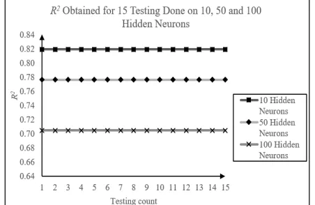
A. Number of Hidden Neurons
The performance of the RBF model obtained using the three different numbers of hidden neurons (10, 50 and 100) is shown in Table V.
TABLE V MSE AND R2 V
ALUES OBTAINED USING DIFFERENT HIDDEN NEURONS IN
THE RBFNEURAL NETWORK
Fig. 3 The MSE values acquired for the 10, 50 and 100 hidden neurons during the 15 testing.
Fig. 4 R2 values obtained for the number of hidden neurons of 10, 50 and
100 during the 15 testings.
Fig. 3 and Fig. 4 show the MSE and R2 values obtained for the 15-testing done using the 10, 50 and 100 hidden neurons. From these graphs, the RBF model produced consistent results throughout the 15 testings for the 10, 50 and 100 hidden neurons used. The best MSE and R2 values obtained are 0.2206 and 0.8191 with 10 hidden neurons. Therefore, the optimal hidden neurons used will be 10 hidden neurons in the following experiments.
No. Combination of Meteorology Data Used Group
1.
Daily minimum temperature, Daily Maximum Temperature, Daily Mean Temperature, Daily Mean Relative Humidity, Daily Mean Wind Speed & Daily Mean Sea Level Pressure
A
2.
Daily minimum temperature, Daily Maximum Temperature, Daily Mean Temperature, Daily Mean Relative Humidity & Daily Mean Wind Speed (Without Daily Mean Sea Level Pressure)
B
3.
Daily minimum temperature, Daily Maximum Temperature, Daily Mean Temperature, Daily Mean Relative Humidity & Daily Mean Sea Level Pressure (Without Daily Mean Wind Speed
C
4
Daily minimum temperature, Daily Maximum
Temperature, Daily Mean Temperature, Daily Mean Wind Speed & Daily Mean Sea Level Pressure (Without Mean Relative Humidity)
5 Daily Mean Relative Humidity, Daily Mean Wind Speed & Daily Mean Sea Level Pressure (Without temperature)
6
Daily minimum temperature, Daily Maximum Temperature & Daily Mean Temperature (Only Temperature)
7 Daily Mean Relative Humidity Only
8 Daily Mean Wind Speed Only
9 Daily Sea Level Pressure Only
10 Daily Mean Relative Humidity and Daily Mean Sea Level Pressure
11 Daily Mean Relative Humidity and Daily Mean Wind Speed
12
Daily minimum temperature, Daily Maximum Temperature, Daily Mean Temperature and Daily Mean Relative Humidity
13
Daily minimum temperature, Daily Maximum Temperature, Daily Mean Temperature and Daily Mean Sea Level Pressure
14 Daily minimum temperature, Daily Maximum Temperature, Daily Mean Temperature and Daily Mean Wind Speed
15 Daily Mean Wind Speed & Daily Mean Sea Level Pressure
No. of hidden neurons MSE R2
10 0.2206 0.8191
50 0.2473 0.7763
B. Training Data Size
Using the 10 hidden neurons, the RBF neural network is next tested on the different training data size as shown in Table III. The results of this part of the experiments are shown in Table VI.
TABLE VI
MSEAND R2VALUES OBTAINED USING DIFFERENT NUMBER
OF TRAINING DATA
Training Data Size MSE R2
Group 1 (12 months) 0.2547 0.7726
Group 2 (24 months) 0.2667 0.7539
Group 3 (36 months) 0.2513 0.7745
Group 4 (48 months) 0.2199 0.8282
Group 5 (59 months) 0.2206 0.8191
Fig. 5 MSE and R2 values obtained using 12, 24, 36, 48 and 59 months of
training data.
From Table VI the MSE values obtained using the increasing number of training data do not show a consistent trend. The network performance in terms of MSE deteriorated as the size of the data for training increased from 12 months to 24 months. However, the performance of the model increased when the data used for training increased to 36 and 48 months. The MSE increased a little as the size of the training data raised to 59 months from 48 months. Due to the inconsistent trend of MSE value and as the increment of MSE is only around 0.32% for 48 and 59 months of training data, the optimum training data size to be used is 59 months.
C. Using Different Combination of Meteorology Data
With 10 hidden neurons and 59 months of training data, the contribution of the different combination of meteorology data (Table IV) as the input variable of the RBF network model is given in Table VII.
From Table VII the best combination of meteorology data was Group C, i.e., Daily minimum temperature, Daily Maximum Temperature, Daily Mean Temperature, Daily Mean Relative Humidity and Daily Mean Sea Level Pressure (without Daily Mean Wind Speed). This is better illustrated using the line graph in Fig. 6. With this combination, the RBF neural network produced MSE of 0.1885 with R2 = 0.8467. The MSE obtained with this combination of meteorology data is 14.5% better as compared when all the six-meteorology data used (MSE = 0.2206, R2 = 0.8191). In addition, it can also be seen that the use of only the Daily Mean Wind Speed produced the worst forecasting result
(MSE = 0.6453, R2 = 0.1997). This is followed using only Daily Sea Level Pressure (MSE = 0.6312, R2 = 0.1501) and combination of Daily Mean Wind Speed & Daily Mean Sea Level Pressure (MSE = 0.5139, R2 = 0.5784). Therefore, it can be concluded that the Daily Sea Level Pressure and Daily Mean Wind Speed are less contributing to predictor variables. The results obtained in Group B of TABLE III (i.e. Daily minimum temperature, Daily Maximum Temperature, Daily Mean Temperature, Daily Mean Relative Humidity & Daily Mean Wind Speed (Without Daily Mean Sea Level Pressure)) with MSE = 0.2207 and R2 = 0.8328 has further verified this.
TABLE VII
MSEAND R2VALUES OBTAINED USING DIFFERENT COMBINATION OF
METEOROLOGY
Group MSE R2
A 0.2206 0.8191
B 0.2207 0.8328
C 0.1885 0.8467
D 0.3416 0.6536
E 0.2575 0.8067
F 0.2580 0.7485
G 0.2338 0.8599
H 0.6453 0.1997
I 0.6312 0.1501
J 0.2090 0.8345
K 0.2282 0.8011
L 0.2598 0.7611
M 0.2831 0.7440
N 0.3450 0.6403
O 0.5139 0.5784
Fig. 6 MSE values obtained using a group of different meteorology data combination as shown in Table III.
IV.CONCLUSION
found were Daily Sea Level Pressure and Daily Mean Wind Speed. Another important observation from this study is that, although the RBF neural network model did not produce consistent MSE and R2 results when different training data size was used, the variance between the values obtained was small when the network model is trained with enough training data. In another word, more training data does not seem to enhance the RBF model’s performance after the network has learned from sufficient data. Therefore, it could be concluded that the main factor affecting the performance of the RBF model is the different combinations of input variables used. The use of the incorrect combination of contributing variables could deteriorate the performance of the network model
ACKNOWLEDGMENT
We would like to thank the Faculty of Computer Science and Information Technology, University Malaysia Sarawak (UNIMAS) for providing the computing facilities to conduct the research. We also would like to express our gratitude to the Department of Irrigation and Drainage (DID) Kuching, Sarawak in providing us with the meteorology data. This research work has been done with the support of UNIMAS Special FRGS 2016 Cycle with the project no: F08/SpFRGS/1528/2017.
REFERENCES
[1] Dou, X., J. Song, L. Wang, B. Tang, S. Xu, F. Kong, and X. Jiang, Flood risk assessment and mapping based on a modified multi-parameter flood hazard index model in the Guanzhong Urban Area, China. Stochastic Environmental Research and Risk Assessment, 2018. 32(4): p. 1131-1146.
[2] Ouma, Y.O. and R. Tateishi, Urban Flood Vulnerability and Risk Mapping Using Integrated Multi-Parametric AHP and GIS: Methodological Overview and Case Study Assessment. Water, 2014. 6(6): p. 1515-1545.
[3] Archer, D.R. and H.J. Fowler, Characterising flash flood response to intense rainfall and impacts using historical information and gauged data in Britain. Journal of Flood Risk Management, 2018. 11(S1): p. S121-S133.
[4] Seejata, K., A. Yodying, T. Wongthadam, N. Mahavik, and S. Tantanee, Assessment of flood hazard areas using Analytical Hierarchy Process over the Lower Yom Basin, Sukhothai Province. Procedia engineering, 2018. 212: p. 340-347.
[5] Termeh, S.V.R., A. Kornejady, H.R. Pourghasemi, and S. Keesstra, Flood susceptibility mapping using novel ensembles of adaptive neuro fuzzy inference system and metaheuristic algorithms. Science of the Total Environment, 2018. 615: p. 438-451.
[6] Lee, J., C.-G. Kim, J.E. Lee, N.W. Kim, and H. Kim, Application of Artificial Neural Networks to Rainfall Forecasting in the Geum River Basin, Korea. Water, 2018. 10(10): p. 1448.
[7] Xingjian, S., Z. Chen, H. Wang, D.-Y. Yeung, W.-K. Wong, and W.-c. Woo. Convolutional LSTM network: A machine learning approach for precipitation nowcasting. in Advances in neural information processing systems. 2015.
[8] Wang, B., J. Lu, Z. Yan, H. Luo, T. Li, Y. Zheng, and G. Zhang Deep Uncertainty Quantification: A Machine Learning Approach for Weather Forecasting. arXiv e-prints, 2018.
[9] Aggarwal, R. and R. Kumar, A Comprehensive Review of Numerical Weather Prediction Models. International Journal of Computer Applications, 2013. 74(18).
[10] Bellier, J., I. Zin, S. Siblot, and G. Bontron. Probabilistic flood forecasting on the Rhone River: evaluation with ensemble and analogue-based precipitation forecasts. in E3S Web of Conferences. 2016. EDP Sciences.
[11] Abbot, J. and J. Marohasy, Forecasting of Medium-term Rainfall Using Artificial Neural Networks: Case Studies from Eastern Australia. Engineering and Mathematical Topics in Rainfall, 2018: p. 33.
[12] Sittichok, K., A.G. Djibo, O. Seidou, H.M. Saley, H. Karambiri, and J. Paturel, Statistical seasonal rainfall and streamflow forecasting for the Sirba watershed, West Africa, using sea-surface temperatures. Hydrological Sciences Journal, 2016. 61(5): p. 805-815.
[13] Tharun, V., R. Prakash, and S.R. Devi. Prediction of Rainfall Using Data Mining Techniques. in 2018 Second International Conference on Inventive Communication and Computational Technologies (ICICCT). 2018. IEEE.
[14] Meyer, H., M. Kühnlein, T. Appelhans, and T. Nauss, Comparison of four machine learning algorithms for their applicability in satellite-based optical rainfall retrievals. Atmospheric research, 2016. 169: p. 424-433.
[15] Cramer, S., M. Kampouridis, A.A. Freitas, and A.K. Alexandridis, An extensive evaluation of seven machine learning methods for rainfall prediction in weather derivatives. Expert Systems with Applications, 2017. 85: p. 169-181.
[16] Chai, S.-S., W.K. Wong, and K.L. Goh, Backpropagation Vs. Radial Basis Function Neural Model: Rainfall Intensity Classification For Flood Prediction Using Meteorology Data. JCS, 2016. 12(4): p. 191- 200.
[17] Broomhead, D.S., Multivariate functional interpolation and adaptive networks. Complex Systems, 1988. 2(3): p. 321-355.
[18] Bakar, M.A.A., F.A.A. Aziz, S.F.M. Hussein, S.S. Abdullah, and F. Ahmad. Flood Water Level Modeling and Prediction Using Radial Basis Function Neural Network: Case Study Kedah. In Asian Simulation Conference. 2017. Springer.
[19] Chang, F.-J., J.-M. Liang, and Y.-C. Chen, Flood forecasting using radial basis function neural networks. IEEE Transactions on Systems, Man, and Cybernetics, Part C (Applications and Reviews), 2001. 31(4): p. 530-535.
[20] Tezel, G. and M. Buyukyildiz, Monthly evaporation forecasting using artificial neural networks and support vector machines. Theoretical and Applied Climatology, 2016. 124(1): p. 69-80. [21] El Shafie, A.H., A. El-Shafie, A. Almukhtar, M. Taha, H.G. El
Mazoghi, and A. Shehata, Radial basis function neural networks for reliably forecasting rainfall. Journal of water and climate change, 2012. 3(2): p. 125-138.
[22] Vivekanandan, N., Prediction of Rainfall Using MLP and RBF Networks. International Journal of Advanced Networking and Applications, 2014. 5(4): p. 1974.
[23] Biswas, S.K., L. Marbaniang, B. Purkayastha, M. Chakraborty, H.R. Singh, and M. Bordoloi, Rainfall forecasting by relevant attributes using artificial neural networks-a comparative study. International Journal of Big Data Intelligence, 2016. 3(2): p. 111-121.
[24] Sa’adi, Z., S. Shahid, T. Ismail, E.-S. Chung, and X.-J. Wang, Trends analysis of rainfall and rainfall extremes in Sarawak, Malaysia using modified Mann–Kendall test. Meteorology and Atmospheric Physics, 2017.
[25] Kim, T., W. Ko, and J. Kim, Analysis and Impact Evaluation of Missing Data Imputation in Day-ahead PV Generation Forecasting. Applied Sciences, 2019. 9(1): p. 204.
[26] Markopoulos, A.P., S. Georgiopoulos, and D.E. Manolakos, On the use of back propagation and radial basis function neural networks in surface roughness prediction. Journal of Industrial Engineering International, 2016. 12(3): p. 389-400.
[27] Moghaddam, A.H., M.H. Moghaddam, and M. Esfandyari, Stock market index prediction using artificial neural network. Journal of Economics, Finance and Administrative Science, 2016. 21(41): p. 89-93
[28] Barati-Harooni, A., A. Najafi-Marghmaleki, and A.H. Mohammadi, A reliable radial basis function neural network model (RBF-NN) for the prediction of densities of ionic liquids. Journal of Molecular Liquids, 2017. 231: p. 462-473.
[29] Wang, Y.-X. and M. Hebert. Learning to Learn: Model Regression Networks for Easy Small Sample Learning. 2016. Cham: Springer International Publishing.