Stochastic Partial Differential Equations
Thesis by Maolin Ci
In Partial Fulfillment of the Requirements for the Degree of
Doctor of Philosophy
California Institute of Technology Pasadena, California
2014
c
Acknowledgments
I would like to express my gratitude to my advisor Professor Yizhao Thomas Hou, who has always provided me with great support and guidance in my work and life. His enthusiasm for knowledge and mathematical rigor is the perfect role model for me during my reach. He has also helped me a lot in overcoming the difficulties in every aspect of my life.
Besides my advisor, I would like to thank the rest of my thesis committee: Pro-fessor James Beck, ProPro-fessor Oscar Bruno, and ProPro-fessor Houman Owhadi, for their encouragement and insightful comments. I would also like to thank the staff of the ACM department - Sydney Garstang, Carmen Nemer-Sirois, and Sheila Shull, for their kind help over the years.
I am grateful to my collaborators and colleagues Zhiwen Zhang, Zuoqiang Shi, Guo Luo, Mulin Cheng, Xin Hu and Peyman Tavallali, for their stimulating discussions and help. I also wish to thank many other friends who made my graduate studies memorable, including Hongchao Zhou, Yu Zhao, Debbie Yu, Da Yang, Xuan Zhang, Sinan Zhao, Jiang Li, Daiqi Linghu, Liling Gu, Molei Tao, and Tong Chen.
Abstract
Partial differential equations (PDEs) with multiscale coefficients are very difficult to solve due to the wide range of scales in the solutions. In the thesis, we propose some efficient numerical methods for both deterministic and stochastic PDEs based on the model reduction technique.
For the deterministic PDEs, the main purpose of our method is to derive an ef-fective equation for the multiscale problem. An essential ingredient is to decompose the harmonic coordinate into a smooth part and a highly oscillatory part of which the magnitude is small. Such a decomposition plays a key role in our construction of the effective equation. We show that the solution to the effective equation is smooth, and could be resolved on a regular coarse mesh grid. Furthermore, we provide error analysis and show that the solution to the effective equation plus a correction term is close to the original multiscale solution.
For the stochastic PDEs, we propose the model reduction based data-driven s-tochastic method and multilevel Monte Carlo method. In the multiquery, setting and on the assumption that the ratio of the smallest scale and largest scale is not too small, we propose the multiscale data-driven stochastic method. We construct a data-driven stochastic basis and solve the coupled deterministic PDEs to obtain the solutions. For the tougher problems, we propose the multiscale multilevel Monte Carlo method. We apply the multilevel scheme to the effective equations and assem-ble the stiffness matrices efficiently on each coarse mesh grid. In both methods, the Karhunen-Lo`eve expansion plays an important role in extracting the main parts of some stochastic quantities.
Contents
Acknowledgments iv
Abstract v
1 Introduction 1
1.1 Background . . . 1
1.2 Literature review . . . 2
1.3 Model reduction . . . 7
1.3.1 Deterministic case . . . 8
1.3.2 Stochastic case with data-driven stochastic method . . . 10
1.3.3 Stochastic case with multilevel Monte Carlo method . . . 11
2 Multiscale model reduction method for elliptic PDEs 14 2.1 Derivation of effective equations . . . 14
2.2 Analysis . . . 15
2.2.1 The one-dimensional case . . . 16
2.2.2 An error estimate for the general case . . . 17
2.3 Comparison with the homogenization method . . . 22
2.4 Numerical Implementation . . . 24
2.4.1 Decomposition of the harmonic coordinates . . . 24
2.4.2 Numerical results . . . 25
3 Multiscale model reduction method for time-dependent PDEs 35 3.1 Effective equations . . . 35
3.1.2 Convection-diffusion equation . . . 36
3.1.3 Hyperbolic equation . . . 36
3.2 Error estimate . . . 37
3.3 Numerical results . . . 42
4 Modified multiscale model reduction method for deterministic PDEs with locally degenerate coefficients 49 4.1 Difficulties with locally degenerate coefficients . . . 49
4.2 Analysis for one-dimensional elliptic PDEs . . . 50
4.3 Generalization to parabolic equations . . . 53
4.4 Numerical results . . . 54
5 Model reduction based multiscale data-driven stochastic method for elliptic PDEs with random coefficients 58 5.1 The Karhunen-Lo`eve expansion . . . 58
5.2 Derivation of model reduction based multiscale data-driven stochastic method . . . 60
5.2.1 Effective stochastic equations . . . 61
5.2.2 Data-driven stochastic basis for the effective stochastic equations 62 5.2.3 Complete algorithm . . . 65
5.3 Computational complexity analysis . . . 67
5.3.1 Computational cost of the SCFEM solver . . . 68
5.3.2 Computational cost of the MsDSM and the DSM solvers . . . 68
5.4 Numerical examples . . . 70
5.4.1 Comparison of the MsDSM and the SCFEM . . . 71
5.4.2 Comparison of the MsDSM and the DSM . . . 78
6 Model reduction based multiscale multilevel Monte Carlo method for elliptic PDEs with random coefficients 83 6.1 Multilevel schemes for the effective stochastic equations . . . 83
6.2 Stiffness matrices assembling . . . 87
6.4 Computational complexity analysis . . . 89
6.4.1 Offline computational cost . . . 89
6.4.2 Online computational cost . . . 90
6.5 Numerical examples . . . 90
7 Conclusions 96
List of Figures
2.1 Example 2.1 - The coefficient a and the exact solution ue . . . 26
2.2 Example 2.1 - The derivative of the function F and g (Nc = 16) . . . . 26
2.3 Example 2.2 - The coefficient a and the exact solution ue . . . 28
2.4 Example 2.2 - The derivative of the function F and g (Nc = 16) . . . . 28
2.5 Example 2.3 - The coefficient a and the exact solution ue . . . 29
2.6 Example 2.3 - The derivative of the function F and g (Nc = 16) . . . . 30
2.7 Example 2.4 - The coefficient a and the exact solution ue . . . 31
2.8 Example 2.4 - The derivative of the function F and g (Nc = 16) . . . . 32
2.9 Example 2.5 - The coefficient a and the exact solution ue . . . 33
2.10 Example 2.5 - The derivative of the function F and g (Nc = 16) . . . . 33
3.1 Example 3.1 - The coefficient a . . . 42
3.2 Example 3.1 - Relative errors of the solution . . . 43
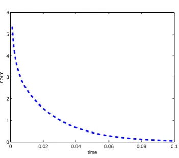
3.3 Example 3.1 - R Ω|∇(˜u0)t| 2dx at N c= 16 . . . 44
3.4 Example 3.2 - The velocity fields u1 and u2 . . . 45
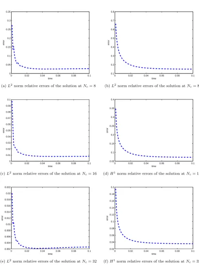
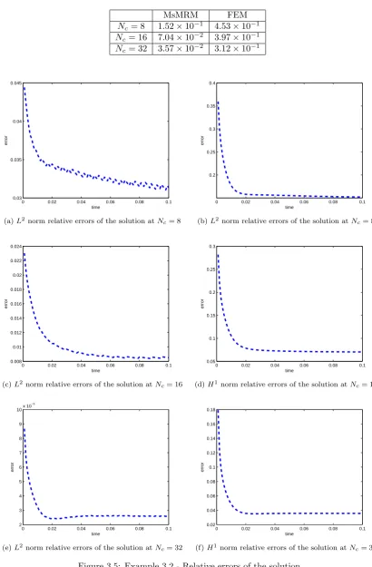
3.5 Example 3.2 - Relative errors of the solution . . . 46
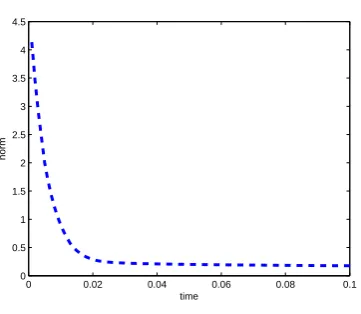
3.6 Example 3.2 - RΩ|∇(˜v0)t|2dx atNc= 16 . . . 47
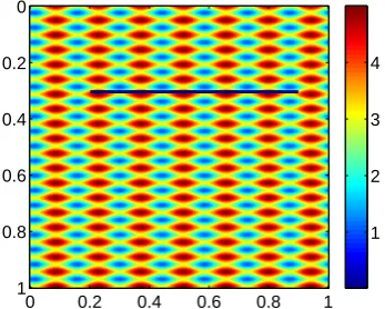
3.7 Example 3.3 - The coefficient a . . . 47
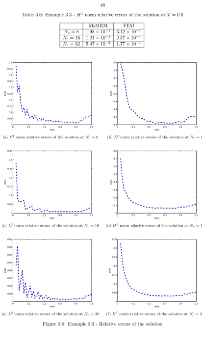
3.8 Example 3.3 - Relative errors of the solution . . . 48
4.1 Example 4.1 - The coefficient a . . . 54
4.2 Example 4.3 - The coefficient a . . . 56
5.1 Greedy stochastic basis enriching algorithm on a coarse-fine grid hierarchy. 63 5.2 Example 5.1 - Some samples of the coefficient a . . . 72
5.4 Example 5.2 - Some samples of the coefficient a . . . 74
5.5 Example 5.3 - κ1, κ2, κ3 and some samples of the coefficient a . . . 77
5.6 Example 5.3 - The computation time comparison . . . 78
5.7 Example 5.4 - Some samples of the coefficient a . . . 79
5.8 Example 5.5 - The computation time comparison . . . 82
6.1 Example 6.2 - Variance decay on the coarse mesh grids . . . 93
List of Tables
2.1 Example 2.1 - L2 norm relative errors of the solution . . . . 27
2.2 Example 2.1 - H1 norm relative errors of the solution . . . . 27
2.3 Example 2.1 - L∞ norm of the function χ . . . 27
2.4 Example 2.1 - L2 norm and H1 norm relative errors of the function g (Nc= 16) . . . 28
2.5 Example 2.2 - L2 norm relative errors of the solution . . . 28
2.6 Example 2.2 - H1 norm relative errors of the solution . . . . 28
2.7 Example 2.2 - L∞ norm of the function χ . . . 29
2.8 Example 2.2 - L2 norm and H1 norm relative errors of the function g (Nc= 16) . . . 29
2.9 Example 2.3 - L2 norm relative errors of the solution . . . 30
2.10 Example 2.3 - H1 norm relative errors of the solution . . . . 30
2.11 Example 2.3 - L∞ norm of the function χ . . . 30
2.12 Example 2.3 - L2 norm and H1 norm relative errors of the function g (Nc= 16) . . . 30
2.13 Example 2.4 - L2 norm relative errors of the solution . . . 31
2.14 Example 2.4 - H1 norm relative errors of the solution . . . . 32
2.15 Example 2.4 - L∞ norm of the function χ . . . 32
2.16 Example 2.4 - L2 norm and H1 norm relative errors of the function g (Nc= 16) . . . 32
2.17 Example 2.5 - L2 norm relative errors of the solution . . . 34
2.18 Example 2.5 - H1 norm relative errors of the solution . . . . 34
2.20 Example 2.5 - L2 norm and H1 norm relative errors of the function g
(Nc= 16) . . . 34
3.1 Example 3.1 - L2 norm relative errors of the solution at T = 0.1 . . . . 44
3.2 Example 3.1 - H1 norm relative errors of the solution at T = 0.1 . . . . 44
3.3 Example 3.2 - L2 norm relative errors of the solution at T = 0.1 . . . . 45
3.4 Example 3.2 - H1 norm relative errors of the solution at T = 0.1 . . . . 46
3.5 Example 3.3 - L2 norm relative errors of the solution at T = 0.5 . . . . 47
3.6 Example 3.3 - H1 norm relative errors of the solution at T = 0.5 . . . . 48
4.1 Example 4.1 - Relative errors of the solution . . . 55
4.2 Example 4.2 - Relative errors of the solution . . . 56
4.3 Example 4.3 - Relative errors of the solution . . . 56
4.4 Example 4.4 - Relative errors of the solution at T = 0.1 . . . 57
5.1 Computational time of the linear equation solver for one collocation point. (Time: Sec.) . . . 68
5.2 Computational time of the offline computation. (Time: Sec.). m=7. . 70
5.3 Computational time of forward/back substitution. (Time: Sec.) m is the basis number. The data marked with an asterisk is obtained by extrapolation. . . 70
5.4 Example 5.1 - L2 and H1 norm relative errors of the mean . . . . 73
5.5 Example 5.1 - L2 and H1 norm relative errors of the STD . . . . 73
5.6 Example 5.2 - L2 and H1 norm relative errors of the mean . . . 75
5.7 Example 5.2 - L2 and H1 norm relative errors of the STD . . . . 75
5.8 Example 5.3 - L2 and H1 norm relative errors of the mean . . . . 76
5.9 Example 5.3 - L2 and H1 norm relative errors of the STD . . . 78
5.10 Example 5.4 - L2 and H1 norm relative errors of the mean . . . . 80
5.11 Example 5.4 - L2 and H1 norm relative errors of the STD . . . 80
5.12 Example 5.5 - L2 and H1 norm relative errors of the solution . . . . 81
6.1 Example 6.1 - L2 norm relative errors of the solution . . . . 91
6.3 Example 6.2 - L2 norm relative errors of the solution . . . . 93
Chapter 1
Introduction
1.1
Background
A broad range of scientific and engineering problems involve partial differential e-quations (PDEs) with multiple scales. Such disparities appear in virtually all areas of modern science and engineering: composite materials, porous media, turbulence transport in high Reynolds number flows, atmosphere/ocean science, finance, and so on. Also, in recent years, there has been an increasing interest in the simulation of systems with uncertainties. Many physical and engineering applications involving uncertainty quantification can be described by stochastic partial differential equa-tions (SPDEs), and another challenge in uncertainty quantification is solving SPDEs involving multiple scales.
For example, the difficulty in analyzing groundwater transport is mainly caused by the heterogeneity of subsurface formations spanning over many scales, and there is no apparent scale separation. We need to solve PDEs to perform some reliable simulations. Consider the following PDE
∇ ·(a(x)∇u(x)) = f(x). (1.1)
flow, the media properties often contain uncertainties. These uncertainties are usually parameterized, and one deals with a large set of permeability fields with a multiscale nature. We are interested in some expected quantities of the solutions, and need to solve the corresponding SPDEs.
Due to the wide range of scales in these solutions, it is extremely challenging to resolve the small scales of the solutions by direct numerical simulation. Tremendous computational resources are required to solve for the small scales of the solution, which makes it prohibitively expensive to solve such problems. Even for today’s computing resources, it is easy to exceed the limit of computer memory or CPU time. Sometimes, from an application perspective, it is often sufficient to predict the macroscopic properties of the multiscale systems, and therefore, we are interested in the large scale solutions. Furthermore, if we want to find out the information at all scales, we can construct the small scale solutions from the large scale solutions by exploring the coupling between them. Thus, finding an effective equation that governs the large scale solution is very important. It is very difficult to derive an effective equation since the coupling between the small scale solution and the large scale solution is in general nonlinear and nonlocal. SPDEs involving multiple scales become more complicated. We not only need to use a very fine mesh to resolve the small scales of the solution in the physical space, but also need to approximate the solution in the stochastic space of which the dimension could be high. Thus, we need to seek accurate numerical methods for PDEs and SPDEs with multiple scales, and reduce the computational cost.
1.2
Literature review
Many multiscale methods have been developed in the literature to solve deterministic and stochastic PDEs. We will discuss some existing numerical methods that are relevant to our model reduction method.
state-space onto a properly chosen low-dimensional subspace to arrive at a smaller system that has properties similar to the original system. Complex systems can thus be approximated by simpler systems involving fewer equations and unknown vari-ables, which can be solved much more quickly than the original problem. Here, we borrow the term ‘model reduction’ and apply it to the multiscale PDEs/SPDEs. Our idea is to construct an effective equation that is similar to the original equation. The new equation governs the large scale information of the solution, and a correction term is easily computed from the large scale solution. Thus, the new equation could be solved by the standard finite element method on a coarse mesh grid. We could use a low-dimensional finite element space to resolve the solution instead of a high-dimensional one, which achieves the purpose of model reduction. Since the solution to the new equation is smooth, we call it the effective equation. However, in general, the coefficients of the effective equations are not as smooth as the solutions. Although the coefficients still have small scale information, we can still solve the effective equation by the finite element method on a coarse mesh grid. In fact, we take the average of the coefficients on the coarse mesh grid when we do integrations through the finite element basis functions. We will see it clearly in Chapter 2.2.
Homogenization (see e.g. [10]) is a powerful tool in understanding the large s-cale behaviour of the system under the assumption of ss-cale separation and periodic structures. When the coefficients have scale separation and are periodic with respect to the fast variable, we can construct the homogenized coefficients. The large scale solution will satisfy the same kind of equation with the new homogenized coefficients. However, this method is strongly restricted by the assumptions of scale separation and periodic structures, which is not always satisfied in the applications. Also, to capture the small scale information, the construction of the correction term is not feasible for numerical implementation, since it requires the same computational cost as the original problem; see [48]. In our method, we seek to find the new ‘homoge-nized’ coefficients without scale separation or periodic structures, and the correction terms are easily computed from the large scale solutions.
fields. This approach is extended by Hou and Wu [37] to general heterogeneities. They construct the multiscale basis functions that satisfy the local multiscale equations, and every solution can be expressed as a linear combination of the local basic functions. They also show that boundary conditions for constructing such basic functions are important for the accuracy of the method. Further techniques are explored to improve the accuracy and efficiency of the method, including the oversampling technique, nonconformal basis, local-global information exchange, special boundary conditions for high contrast problems, spectrum decomposition of the space, and so on; see [38, 27, 14, 24, 25, 18, 22] for reference. As we mentioned, the boundary conditions for the basis functions are essential in the methods, and also become a constraint for some problems. The basis functions are local, so the boundary conditions are not easily determined beforehand. Unlike their methods, we use global harmonic coordinates which can be approximated on a fine mesh grid whose computational cost is no more than constructing the local basis functions.
Another method that uses the concept of basis functions is the multiscale finite volume method proposed by Jenny et al. [40, 33]. It is based on the finite volume method rather than the finite element method. They also introduce the bubble func-tion to improve accuracy. We notice that both the multiscale finite element method and multiscale finite volume method use some kind of basis functions, and the con-structions are purely numerical. For the model reduction method, we build a new effective equation without the need for constructing local multiscale basis functions. We point out that any standard numerical method can be applied to our new equa-tion. Our method provides both a theoretical and numerical understanding of the multiscale problem.
The metric based upscaling method proposed by Owhadi et al. [51, 52] shares some common features with our model reduction method. They use the harmonic coordinate to construct a multiscale basis and prove convergence of their multiscale method under some mild conditions on the coefficients (see also [1, 3] for more discus-sions on harmonic coordinates). Specifically, they transform a standard linear finite element basis in the harmonic coordinates to a multiscale basis in the physical coor-dinates. The solution can be well represented by the multiscale basis. However, this method requires the harmonic mapping to be invertible. The numerical implementa-tion of their method is more complicated than ours, since the coarse mesh grid in the metric based upscaling method is severely deformed due to the transformation of the harmonic mapping. In our approach, we are interested in deriving a global upscaling equation. Moreover, we do not require the harmonic mapping to be invertible, and our effective equation can be solved by the standard finite element method on a reg-ular coarse mesh grid. This makes our method easier to implement, and also more efficient.
Among other methods for deterministic PDEs with multiple scales, there are the following: the variational multiscale method by Hughes et al. [39], the heterogeneous multiscale method [21] by E et al., the domain decomposition method by Graham et al. [31, 28], the multiscale finite element method for numerical homogenization by Allaire et al. [2], the multiscale mortar mixed finite element method by Arbogast et al. [4], finite point method by Han et al. [34], and so on. We will not list all the details of the methods; instead, we will switch to reviewing the numerical methods for SPDEs.
sys-tem becomes very large. Both computational cost and memory consumption become prohibitively expensive.
The Wiener chaos expansion or the generalized polynomial chaos (gPC) method [42, 36, 56, 58, 59, 55, 49, 45] employ truncated expansions on a set of polynomial chaos basis functions and drive a system of coupled deterministic PDEs. In the past decade or so, a lot of progress has been made in developing an effective gPC type of methods to solve SPDEs arising from various applications. However, this type of methods still suffers from the curse of dimensionality in the sense that the total number of polynomial chaos basis functions grows quickly as the number of independent random variables becomes larger and larger.
The stochastic collocation method [57, 7, 44] has been developed from the non-intrusive deterministic collocation method and sparse grid techniques. In principle, the stochastic collocation method uses multivariate polynomial interpolations for the integral in the variational formulation of the stochastic system with respect to prob-ability space. A deterministic sequence of points resulting from tensor products of one-dimensional quadrature points is sampled. The exact locations of such points and weights associated with them depend on underlying probability distributions. More-over, hierarchical construction of a generalized sparse grid has also been developed for the application of the stochastic collocation method.
We can see that the so-called curse of dimensionality is one of the essential chal-lenges in the uncertainty quantification. Recently, a data-driven stochastic method [15, 60] was proposed by constructing a problem-dependent stochastic basis to solve these SPDEs. The SPDEs enjoy a compact representation for a broad range of forcing functions under such a stochastic basis. We will solve a number of coupled deter-ministic PDEs by projecting the stochastic solution onto the data-driven stochastic basis and obtain the desired quantities. However, when the coefficients have multiple scales, fine mesh grids are needed to resolve the small scale information, and the cor-responding large coupled system makes it very difficult to solve. Thus, we combine the data-driven basis idea with the model reduction technique, and greatly reduce the computational cost by considering the effective equations on coarse mesh grids.
solv-ing SDEs arissolv-ing in mathematical finance [32]. Similar ideas have been introduced by Heinrich for finite-dimensional parametric integration and solving integral equations [35]. Later, the MLMC method was extended to solve elliptic PDEs with random coefficients; see [9, 19]. The MLMC method is very effective when the solutions to SPDEs are smooth. However, if the solutions of SPDEs possess multiscale features, a naive application of MLMC does not give very good performance, since the asymp-totic variance reduction between two consecutive levels is not valid at the coarse grids unless we make the coarse grids fine enough to resolve the smallest scale feature of the solution. In [19], the authors remark that, the optimal choice for the coarsest level is that the coarsest mesh size should be slightly smaller than the correlation length of the random field, which becomes a major limitation for the method. We will apply the multilevel scheme to the effective equations, and design an efficient numerical method to alleviate the difficulty.
Some other numerical approaches have been proposed to solve SPDEs by explor-ing the sparse structure of the solutions; e.g., the dynamically bi-orthogonal method [16, 17] by Cheng et al. Also, Zabaras et al. propose a stochastic variational mul-tiscale method for diffusion in heterogeneous random media [5, 29]. They combined the generalized polynomial chaos method with the variational multiscale method to achieve model reduction. However, when the dimension in stochastic direction is large, this method is inefficient due to the exponential growth of the number of the gPC basis elements.
1.3
Model reduction
1.3.1 Deterministic case
We use the following elliptic equation as an example to illustrate the main idea of the model reduction approach:
−∇ ·(a(x)∇u(x)) =f(x), x∈D,
u(x) = 0, x∈∂D,
(1.2)
where D ∈ Rd is a spatial domain. The multiscale information is described by the
coefficient a(x). We assume that f(x) ∈ L2(D) is smooth, and a(x) ∈ L∞(D) is
a symmetric, positive definite matrix satisfying λmin(x) ≥ γ > 0 (λmin(x) is the
smallest eigenvalue of a(x)) for a.e. x ∈ D. For such coefficients, the solutions are only H¨older continuous. Ifahas multiple scales, the solution will have multiple scales as well.
We would like to design an effective equation in the following form
−∇ ·(a∗(x)∇u∗(x)) =f(x), x∈D,
u∗(x) = 0, x∈∂D.
(1.3)
formally expand ˜u around g by assuming that χ is small. By taking the leading order terms and substituting them into the original equation, we obtain an effective equation of form (1.3) after ignoring the high order terms involving χ. The effective coefficient a∗ is defined in terms of a, g, andχ as following
a∗(x) = a(x)(I +∂χ
∂x(x)) ∂x
∂g(x), (1.4)
where I is the identity matrix.
We can show that the effective equation derived by the above formal analysis indeed has the desirable smoothness property. Under some conditions, we will show that the solution to the effective equation is inH2, which is one order smoother than
the original multiscale solution. Thus, we can solve the effective equation on a coarse mesh. Moreover, we can show that the error term is small in theH1 norm under some
conditions. From our derivation, we can see that the decomposition of the harmonic coordinates determines the effective coefficient, a∗. An optimal effective coefficient will determine an optimal decomposition. The relationship between these two terms helps us to design a nearly optimal decomposition of F.
on a fine mesh at the subsequent time steps.
1.3.2 Stochastic case with data-driven stochastic method
We propose a multiscale data-driven stochastic method to perform model reduction in both the stochastic and physical spaces. Our new method consists of offline and online stages. In the offline stage, we first derive an effective stochastic equation that can be resolved on a coarse grid. We then construct a data-driven stochastic basis under which the solutions of the effective stochastic equation have a compact representation for a broad range of forcing functions. We consider the following elliptic SPDE with multiscale random coefficients in the multiquery setting
−∇ ·(a(x, ω)∇u(x, ω)) =f(x), x∈D, ω∈Ω,
u(x, ω) = 0, x∈∂D, ω ∈Ω.
(1.5)
whereD ∈Rd is a spatial domain, and Ω is a sample space. The multiscale
informa-tion is also described by the coefficient matrixa(x, ω). We assume thatf(x)∈L2(D) is smooth and a(x, ω) ∈ L∞(D) is a symmetric, positive definite matrix satisfying
λmin(x, ω)≥ γ >0 (λmin(x, ω) is the smallest eigenvalue of a(x, ω)) for a.e. x ∈ D,
ω ∈Ω. We would like to derive a similar effective stochastic equation in the following form
−∇ ·(a∗(x, ω)∇u∗(x, ω)) = f(x), x∈D, ω ∈Ω,
u∗(x, ω) = 0, x∈∂D, ω ∈Ω.
(1.6)
com-pact parametrization for the effective coefficient a∗(x, ω), and a problem-dependent compact basis to represent the stochastic solutions to the effective equation (1.6).
In the first part, we compute the truncated Karhunen-Lo`eve expansion of the ma-trix a∗(x, ω). This compact representation of the effective coefficient enables us to generate a∗(x, ω) very efficiently in the online stage. In the second part, we construct a data-driven stochastic basis by applying the data-driven stochastic method [15] to the effective equation (1.6). We first choose a set of forcing functions and solve (1.6) with one forcing function. Then, we use the Karhunen-Lo`eve expansion of the solu-tion to construct the stochastic basis{Bi(ω)}mi=0. An error analysis is used to evaluate
the completeness of the data-driven basis{Bi(ω)}mi=0. A greedy-type algorithm
com-bined with a two-level preconditioning [20] is used to reduce the computational cost. First, we solve the error equation on the coarse grid for each trial function fk(x),
k = 1,2,· · · , K. We identify the trial function fk∗, which gives the maximum error
and solve the error equation again with this trial function on the fine grid. After that, the Karhunen-Lo`eve expansion of the residual error can be used to enrich the stochastic basis. This process is repeated until the maximum residual error is be-low the prescribed threshold . When this updating process terminates, we obtain a compact data-driven basis {Bi(ω)}mi=0 for the effective stochastic equation (1.6),
which applies to all forcing functions. The detailed implementation of this enriching algorithm depends on specific numerical representation of the stochastic basis, which will be elaborated in detail in Chapter 5.
In the online stage, we expand the solution of (1.6) in terms of the data-driven stochastic basis, and solve a set of coupled deterministic PDEs to obtain the solutions. As in the deterministic case, since we need to solve the equation many times with different forcing functions but the same coefficients, our method in the online stage offers considerable computational savings.
1.3.3 Stochastic case with multilevel Monte Carlo method
ex-pensive, and the online coupled system might become bigger and bigger. In this case, we need to find a more efficient method. We again consider the same elliptic SPDE (1.5), and we are interested in the expected value of some functional of the solutions, which could be the mean and high-order moments. In general, we could approximate the expectations by the standard Monte Carlo method. For the multiscale problems, we must choose the mesh size to be fine enough to control the bias error. Also, many realizations are required to reduce sampling errors.
We have already proven that the solution to the effective equation is a good approx-imation of the original solution. Thus, we could approximate the effective solution and pick the mesh grid much coarser than the original fine mesh grid, which would save a large amount of computational time a lot for each realization.
To further reduce the computational cost, we apply the multilevel scheme proposed in [32] to the effective equation. We first divide the physical domainDinto a number of nested coarse mesh grids, i.e., Dh0 ⊂. . .⊂Dhl−1 ⊂Dhl. . .⊂DhL. Here, hl is the l-th level mesh size (l = 0,1, . . . , L) and h0 is the coarsest level mesh size. Denote
E[u∗l(x, ω)] = E[u
∗
hl(x, ω)] to be the mean of the numerical solution on mesh size hl;
linearity of the expectation operator implies that
E[u∗L(x, ω)] =E[u
∗
0(x, ω)] +
L
X
l=1
E[u∗l(x, ω)−u
∗
l−1(x, ω)]. (1.7)
The key point is to avoid estimating E[u∗L(x, ω)] on the finest level, but instead to estimate it on the coarsest level. The reduction in cost associated with the multilevel Monte Carlo method over the Monte Carlo method is due to the fact that most of the uncertainty can be captured on the coarse grids (h >> hL), so the number of
realizations needed on the grid (h=hL) is greatly reduced due to the variance
reduc-tion between two consecutive grids. We will show the computareduc-tional cost reducreduc-tion by several numerical examples.
Chapter 2
Multiscale model reduction
method for elliptic PDEs
2.1
Derivation of effective equations
In this chapter, we consider the elliptic equation
−∇ ·(a(x)∇u(x)) =f(x), x∈D,
u(x) = 0, x∈∂D.
(2.1)
Let F(x) = (F1(x), ..., Fd(x)) be the harmonic coordinate associated to (2.1) in
d-dimensional space. Then Fk (k = 1, ..., d) satisfies the following elliptic equation
−∇ ·(a(x)∇Fk(x)) = 0, x∈D
Fk(x) = xk, x∈∂D,
(2.2)
wherex= (x1, ..., xd). Write ˜u0 =u◦F−1. It is known that the solutionuis smooth in
terms of the harmonic coordinates, i.e. ˜u0 is inH2. If we could make a decomposition
F =g+χ such thatg is smooth and χis small with zero boundary conditions, then we obtain by applying a formal Taylor expansion to ˜u0 and ignoring the high order
terms,
˜
Letu0(x) = ˜u0(g(x)), then we get
u(x) = ˜u0(F)≈u0(x) +χT
∂x
∂g∇u0(x). (2.4)
Furthermore, we have
∇u(x)≈ ∇u0(x) +
∂χ ∂x
∂x
∂g∇u0(x) +χ
T∇
(∂x
∂g∇u0(x)). (2.5)
By substituting (2.5) into (2.1) and eliminating the high order terms involving O(χ), we get a new PDE for u0
−∇ ·(a(x)(I+∂χ∂x∂x∂g)∇u0(x)) =f(x), x∈D,
u0(x) = 0, x∈∂D,
(2.6)
where I is the identity matrix.
We will show that u0 is in H2 so that we can solve the effective equation (2.6)
accurately on a coarse mesh. Moreover, we will show that the H1 norm of the error,
u−(u0+χT ∂x∂g∇u0), is small. Thus we can approximate u by u0+χT ∂x∂g∇u0 with a
reasonable accuracy. This suggests the following steps of the model reduction method. 1. Solve the harmonic coordinate (2.2) on a fine mesh to get F.
2. DecomposeF =g+χ, hereg is smooth and χ is small with χ= 0 on∂Ω. 3. Solve the effective equation (2.6) on a coarse mesh to getu0.
4. Approximate u by u0+χT ∂x∂g∇u0.
The first and second steps are offline steps. We can store the necessary information so that we can compute u0 efficiently for differentf. The remaining online steps can
be solved very efficiently on a coarse mesh. So far we have not defined what we mean by g being ‘smooth’ and χ being ‘small’. We will discuss the guideline in defining g
and χ, and give one effective construction in the next sections.
2.2
Analysis
In this section, we will perform error analysis to show that the H1 norm of the
that the L∞ norm of χ is small. We will also prove that the solution to the effective equation is in H2 under some conditions. Before presenting the general analysis, we will start with the simple 1-dimensional elliptic equation to illustrate the main idea.
2.2.1 The one-dimensional case
Consider the one-dimensional elliptic equation on a unit interval [0,1]
(a(x)u0(x))0 =f(x), x∈(0,1),
u(0) =u(1) = 0.
(2.7)
The corresponding harmonic coordinate F is defined as
(a(x)F0(x))0 = 0, x∈(0,1),
F(0) = 0, F(1) = 1.
(2.8)
Our effective equation is given by
a(x)F0(x)(u00(x)/g0(x))0 =f(x), x∈(0,1), u0(0) =u0(1) = 0.
(2.9)
We can solve these equations analytically and get
u(x) =C0
F(x)
Z x
0
f(s)ds−
Z x
0
F(s)f(s)ds+C1F(x)
, (2.10)
F(x) = 1
C0
Z x
0
ds
a(s), (2.11)
u0(x) =C0
g(x)
Z x
0
f(s)ds−
Z x
0
g(s)f(s)ds+C2g(x)
where
C0 =
Z 1
0
ds
a(s), (2.13)
C1 =−
Z 1
0
f(s)ds+
Z 1
0
F(s)f(s)ds, (2.14)
C2 =−
Z 1
0
f(s)ds+
Z 1
0
g(s)f(s)ds. (2.15)
Since f ∈ L2 and g is smooth, we can see that u0 is smooth. Let u1 = χu00/g
0
, direct computations give
(u−u0−u1)0 =C0((C1−C2)F0−χf). (2.16)
We also have
C1−C2 =
Z 1
0
χ(s)f(s)ds, (2.17)
and
F0 = 1
C0
1
a(x). (2.18)
By the assumption a(x)≥γ > 0, we know that F0 is bounded. Thus we can bound
ku−u0 −u1kH1 in terms of kχkL∞. This implies that as long as we can decompose
F so that the oscillatory part χ is small and g is smooth, then ku−u0 −u1kH1 is
small and we can solve u0 on a coarse grid. In the next section, we will show that
this result is true for general multi-dimensional elliptic equations as well.
2.2.2 An error estimate for the general case
The main result of this section is the following theorem.
Theorem 2.1. Suppose u, F and u0 are weak solutions to (2.1), (2.2) and (2.6)
respectively. Let u1 =χT ∂x∂g∇u0, F =g+χ, and χ= 0 on ∂Ω. Then we have
ku−u0−u1kH1(D)≤CkχkL∞(D)k
∂g
∂xkL∞(D)kdet( ∂x
∂g)kL∞(D)|u˜0|H2(D), (2.19) where C is a constant that depends on d, D and a, u˜0 =u0◦g−1.
Our goal is to estimate the H1 norm of z = u −u
condition of χ implies the zero-boundary condition of z, i.e. z ∈H1
0(Ω). Since a is a
positive definite matrix whose eigenvalues have a positive lower bound, we conclude that ||z||H1
0(Ω) is equivalent to the energy norm, < a∇z,∇z >, where< . > is the L
2
inner product. Thus, it is sufficient to perform our estimate using the energy norm.
Proof. Define
z =u−u0−u1 ∈H01(D),
p=a∇u−a∂F ∂x
∂x ∂g∇u0,
η=−a ∂ ∂x
∂x ∂g∇u0
χ.
Then we have
∇ ·p=∇ ·(a∇u)− ∇ ·(a∂F ∂x
∂x
∂g∇u0) = f−f = 0, (2.20)
and
a∇z−p=a∇u−a∇u0−a∇u1−a∇u+a
∂F ∂x
∂x
∂g∇u0 =a ∂χ ∂x
∂x
∂g∇u0−a∇u1.
Further, we note that
∇u1 =
∂χ ∂x
∂x
∂g∇u0+ ∂ ∂x
∂x ∂g∇u0
χ.
As a result, we get
a∇z−p=−a ∂ ∂x
∂x ∂g∇u0
χ=η.
Thus, we obtain
< a∇z,∇z >=
Z
D
∇z·a∇zdx
=
Z
D
(a∇z−p)· ∇zdx+
Z
D
p· ∇zdx
=
Z
D
η· ∇zdx−
Z
D
(∇ ·p)zdx
=
Z
D
where we have used (2.20). By using the ellipticity assumption ofa, we get
C1k∇zk2L2(D) ≤< a∇z,∇z >≤ kηkL2(D)k∇zkL2(D),
which implies
C1k∇zkL2(D) ≤ kηkL2(D).
Since z vanishes on∂D, Poincar´e’s theorem gives
kzkH1
0(D) ≤C2k∇zkL2(D).
Thus, we get
kzkH1
0(D) ≤CkηkL2(D),
where C is a constant that depends on d, D and a only. Let y=g(x) and ˜u0(y) = ˜u0(g(x)) =u0(x), then we have
η=−a ∂ ∂x
∂x ∂g∇u0
χ
=−a∂g ∂x
∂x ∂g
∂ ∂x
∂x ∂g∇u0
χ
=−a
∂g ∂x∇
2
yu˜0
χ.
As a result, we obtain
kηkL2(D) ≤CkakL∞(D)kχkL∞(D)k
∂g
∂xkL∞(D)kdet( ∂x
∂g)kL∞(D)|u˜0|H2(D).
The determinant of ∂x
∂g enters the last step of the above estimate due to a change of
variables from x to y. Combining all the results, we get
kzkH1
0(D)≤CkχkL∞(D)k
∂g
∂xkL∞(D)kdet( ∂x
∂g)kL∞(D)|u˜0|H2(D).
This completes the proof of Theorem 2.1.
sense that both k∂g
∂xkL∞(D) andkdet( ∂x
∂g)kL∞(D) are bounded, then the approximation
is accurate provided that |u˜0|H2(D) is bounded. To evaluate |u˜0|H2(D), we make a
change of variables from xto y=g(x) in equation (2.6), which has a non-divergence form
− n
X
i,j=1
Bij(y)
∂2u˜ 0
∂yi∂yj
= ˜f(y), (2.21)
where
B(y) =
|det(∂x
∂g)|( ∂g ∂x) T a∂F ∂x
◦g−1(y) (2.22)
and
˜
f(y) =
|det(∂x
∂g)|f
◦g−1(y). (2.23)
Note that the determinant term comes from the change of variables in the integral since we consider weak solutions.
If the matrix B satisfies the Cordes condition (see e.g. [46]),
Pn
i,j=1Bij2(y)
(Pn
i=1Bii(y))2
≤ 1
n−1 +, (2.24)
for some >0 and M = sup( Pn
i=1Bii(y)
Pn
i,j=1Bij2(y)
)< ∞, we can apply Theorem 1.2.1 in [46] to conclude that
|u˜0|H2(D) ≤
M
1−√1−kfkL2(D). (2.25)
In general, the condition (2.24) is hard to verify. For d = 2, we have a more concrete version for and M. Suppose λmax(y) and λmin(y) are the maximum and
minimum eigenvalues of B(y), ifη1 = sup
λmax(y)
λmin(y) <∞ and η2 = infλmin(y)>0, then
we can pick = η11 and M = η21 .
Remark 2.1. Theorem 2.1 is an error estimate for the analytical solutions. One should not use it to study the convergence rate of the numerical method. It does not imply that the smaller kχkL∞(D) is, the smaller the numerical error would become.
On one hand, if we chooseχ to be 0, in which caseg =F, the error is zero in theory. However, g is no longer smooth and we will have to use a fine mesh to solve the effective equation, which is not what our method is designed for. Similarly, if we let
this case, we will not be able to obtain a small overall error if we use a coarse mesh. From a view point of numerical implementation, it is usually the case thatF may become degenerated in some localized region. The ‘smoothness’ of g depends on the size of the numerical grid. To avoid degeneracy in constructing g, we can use a finer mesh locally to capture some important information in certain local regions, and use a coarser mesh in other regions. By doing this,g is smooth when using a non-uniform mesh, and we can guarantee that χ is small. Choosing an optimal decomposition which would lead to the smallest overall error requires a delicate balance in our decomposition of F. We will discuss more about this issue later.
Remark 2.2. In our analysis, we choose the homogeneous boundary condition. We can still apply our method to nonhomogeneous boundary conditions, as long the the boundary values are smooth, although we do not have the convergence analysis due to the technical reason. When we use the finite element method, we can approximate the boundary values by directly using the finite element basis functions on the boundary. We do not need to transform the nonhomogeneous problem to the homogeneous one by subtracting some function which has the given boundary values, since it will make the new forcing term nonsmooth.
Remark 2.3. The solution in equation (2.6) is in H2, which is one order smoother than the original solution, and that is why we call it the effective equation. However, the coefficient a∗ =a∂F∂x∂x∂g is not smooth in general. For one-dimensional problems,
a∗ =aF0/g0, andaF0 is a constant according to our previous analysis. In this case,a∗
is smooth sincegis smooth. For high dimensional problems,a∂F∂x is no longer constant, so a∗ is not smooth. By the Cordes condition, we know that the smoothness of u0
comes from the fact that we can rewrite equation (2.6) in a non-divergence form. To be more specific, the term a∂F∂x is divergence free, so we have a non-divergence form of equation (2.6).
do integrations through the finite element basis functions.
2.3
Comparison with the homogenization method
In this section, we compare our method with the classical homogenization method. First we briefly review the homogenization theory [10]. Consider
−∇ ·(a(x)∇u(x)) =f(x), x∈D,
u(x) = 0, x∈∂D,
(2.26)
where a(y) is a symmetric, positive definite matrix, andf ∈L2. Furthermore, a
ij(y)
are periodic smooth functions in y in a unit cube Y. The homogenized coefficients are given by
a∗ij = 1
|Y|
Z
Y
aik(y)(δkj+
∂ ∂yk
χjh)dy, (2.27)
whereχjh(we use the notationχjhto distinguish fromχj) is the solution to the periodic cell problem
∇y ·(a(y)∇yχjh(y)) =−
∂ ∂yi
aij(y) (2.28)
with zero mean, i.e. RY χjhdy= 0.
Let u0 be the solution to the homogenized equation
−∇ ·(a∗(x)∇u0(x)) =f(x), x∈D,
u0(x) = 0, x∈∂D.
(2.29)
Then we have
||u−u0||L2(D)≤C||u||H2(D). (2.30)
Further, we define
u1(x) =χjh(
x )
∂u0
∂xj
(x). (2.31)
satisfying
−∇ ·(a(x)∇θ(x)) = 0, x∈D,
θ(x) =u1, x∈∂D.
(2.32)
Then it can be shown that (see e.g. [48])
||u−u0−(u1−θ)||H1(D) ≤C||u0||H2(D). (2.33)
The constant C is independent of u0 and .
One important advantage of our method is that we can take care of a continuum of scales and do not require periodicity on the microstructure while homogenization theory usually requires scale separation and periodic structures. Moreover, one must include a boundary correction term θ to achieve H1 convergence in the
homoge-nization method. This correction term must be solved on a fine mesh grid and is expensive to compute. In comparison, there is no need to compute a correction term in our method since we requireχ= 0 on ∂D.
If only L2 convergence is needed, both methods do not need correction terms, and the homogenized coefficients are easier to compute (see (2.27) and (2.28)). Our method requires two global solutions on a fine mesh. However, under the conditions for homogenization (periodic smootha(y)), we can modify our method easily so that we can compute the harmonic coordinates with the same cost as the homogenization method. Specifically, the harmonic coordinate F satisfies ∇ ·(a(x
)∇F(x)) = 0 and
F =g+χ. If we set g =x, we get the equation for χ as follows
∇ ·(a(x
)∇χ
j
(x)) =−1
∂ ∂yi
aij(
x
). (2.34)
Now we do not require χ = 0 on the boundary, assume χj to be periodic in Y and
impose the constraint RY χj(x)dx= 0. Equation (2.34) is still global, but comparing (2.34) with (2.28) gives χ(x) = χh(x). So we can solve (2.28) instead of (2.34).
2.4
Numerical Implementation
2.4.1 Decomposition of the harmonic coordinates
In this section, we discuss how to construct the decomposition of the harmonic coor-dinates. As we know from the previous sections, the decomposition F =g+χ plays an essential role in our method. Here we discuss some guidelines in choosing such a decomposition and how to construct it numerically.
The first criterion in choosing our decomposition is to make sure that g is smooth and invertible. We need to define what we mean byg being smooth. The smoothness is relative to the coarse mesh that we will use to solve the effective equation. In our numerical implementation, we use the standard linear finite element method to solve the effective equation. Thus, any linear combination of the nodal basis on the coarse mesh could be considered as a smooth function, and we can chooseg in this form.
The second criterion of our decomposition is to make χ small. If we choose the nodal values of g close to those of F, then we expect that the difference between the two would be small. This suggests a natural way to define g, i.e. we can choose the nodal values of g at the coarse mesh points to be the same as F at these coarse mesh points. We can then interpolateg from the coarse mesh points to the fine mesh points using the linear interpolation. Once we have defined g globally through linear interpolation, we have also determinedχ=F −g. Since F is linear on the boundary, such decomposition guarantees thatg =F on the boundary, which implies thatχ= 0 on∂D.
We also have another guideline to determine whether the decomposition is effective or not from the view point of numerical implementation. Note thatug =g solves the
following equation exactly:
−∇ ·(a(x)(I+ ∂χ∂x∂g∂x)∇ug(x)) = 0, x∈D,
ug(x) =x, x∈∂D.
(2.35)
ug and g to determine whether we obtain a good decomposition for F. The smaller
the difference is, the better the method would perform.
2.4.2 Numerical results
We perform several numerical experiments to test our multiscale model reduction method (MsMRM) for the elliptic equation (2.1). We take D = [0,1]×[0,1] in 2-dimensional space. Since it is difficult to construct a general enough test problem with an analytic solution, we use well resolved numerical solutions in place of exact solutions. In our computations, we use the standard linear finite element method (FEM). We compare the solution on a 256×256 mesh and a 512×512 mesh. The
L2 relative error is less than 1×10⁻³ and the H1 relative error is less than 2×10⁻².
So the numerical solution on the 256×256 mesh is well resolved by the mesh and we can consider it as the reference solution. To implement our method, the coarse meshes are chosen to be 8×8, 16×16 and 32×32 respectively, and we compare the results on different meshes. As we mentioned, the forcing terms should be resolved by the coarse mesh, so we choose f(x, y)∈ {sin(kiπx+li) cos(miπy+ni)}i∈J, where ki, li,mi, andni are random numbers uniformly distributed over the interval [0,0.5].
We also choose the FEM as the benchmark and compare our method with it.
Example 2.1. We consider the case when the elliptic coefficient is a scalar defined by
a(x, y) = 1
2 + 1.6 sin(2π(x−y)/1)
+ 1
4 + 1.8(sin(2πx/2) + sin(2πy/2))
+ 1
10(2 + 1.8 sin(2π(x−0.5)/3))(2 + 1.8 sin(2π(y−0.5)/3))
,
where 1 = 13, 2 = 111, 3 = 191.
In this example,f(x, y) = sin(0.48πx+ 0.17) cos(0.29πy+ 0.11). In Figure 2.1-2.2, we plot the coefficient and the decomposition. Relative errors are shown in Tables 2.1 and 2.2. From these figures, we can see that the coefficient oscillates very rapidly, which generates small scale features in the solution (e.g. ∂F1∂x1). The smooth part of
Theorem 2.1 are satisfied. We observe convergence in both L2 and H1 norms.
0 0.2 0.4 0.6 0.8 1
0 0.2 0.4 0.6 0.8 1 1 2 3 4 5 6 (a)a
0 0.2 0.4 0.6 0.8 1
0 0.2 0.4 0.6 0.8 1 0 0.01 0.02 0.03 0.04
(b)ue
Figure 2.1: Example 2.1 - The coefficientaand the exact solutionue
0 0.2 0.4 0.6 0.8 1
0 0.2 0.4 0.6 0.8 1 0.6 0.8 1 1.2 1.4 1.6 1.8
(a) ∂F1
∂x1 (Nc= 16)
0 0.2 0.4 0.6 0.8 1
0 0.2 0.4 0.6 0.8 1 0.7 0.8 0.9 1 1.1 1.2 1.3 1.4
(b) ∂g1
∂x1 (Nc= 16)
Figure 2.2: Example 2.1 - The derivative of the functionF andg (Nc= 16)
Remark 2.4. We remark that Theorem 2.1 does not give a specific rate of con-vergence. It is worthwhile to make the following observations on the convergence property of our method. Denote the exact solution as ue, the solution constructed
from the effective equation as um and its numerical approximation as un. Then the
error consists of two parts, i.e. ||ue−um||+||um−un||. The first part is controlled
by Theorem 2.1, and it gets smaller as we use a finer size. For fixed um, the second
part converges at order O(h2) (L2 norm) or order O(h1) (H1 norm). However, as
Table 2.1: Example 2.1 -L2 norm relative errors of the solution
MsMRM FEM
Nc= 8 2.58×10⁻² 1.16×10⁻¹ Nc = 16 7.27×10⁻³ 6.60×10⁻² Nc = 32 3.45×10⁻³ 3.58×10⁻²
Table 2.2: Example 2.1 -H1 norm relative errors of the solution
MsMRM FEM
Nc= 8 1.67×10⁻¹ 3.31×10⁻¹ Nc = 16 8.26×10⁻² 2.44×10⁻¹ Nc = 32 4.00×10⁻² 1.74×10⁻¹
the overall rate of convergence is not necessarily O(h2) or O(h1). In all our
numer-ical experiments, we observe different rates of convergence for different mesh sizes, especially for the L2 norm. On the finest mesh, the error will eventually converge to zero (if we take the numerical solution on the finest mesh to be the true solution). However, we want to perform our method on a coarse mesh instead of a fine one. Our main objective is not to find the optimal convergence rate, but to reduce the error on a given coarse mesh. So we are more interested in the error itself rather than the convergence rate. It is important not to be confused with these two issues.
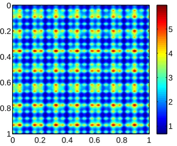
Example 2.2. We choose an anisotropic field a as a(x, y) = |θ(x, y)|+ 0.5. Here
θ(x, y) is defined on a 23×23 grid over the domain D, and for each grid cell, the value of θ(x, y) is distributed according to the standard normal distribution (see Figure 2.3a). The multiscale coefficient, a, is very rough and does not satisfy scale separation or have any periodic structure. Compared with the first example, both the coefficient and the solution are more singular. This presents a challenging test problem for our method. In this example, f(x, y) = sin(0.33πx+ 0.43) cos(0.43πy+ 0.38). As we can see from the error study presented in Table 2.5-2.6, our method still gives a satisfactory convergence rate and the relative errors are quite small.
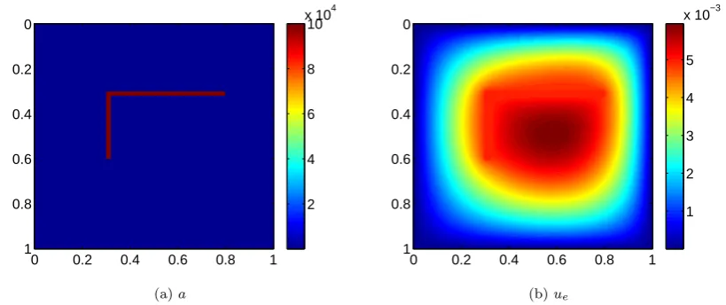
Example 2.3. Next, we consider an example that has a discontinuous and high
Table 2.3: Example 2.1 -L∞ norm of the functionχ
χ1 χ2
Table 2.4: Example 2.1 -L2 norm andH1 norm relative errors of the functiong(Nc= 16)
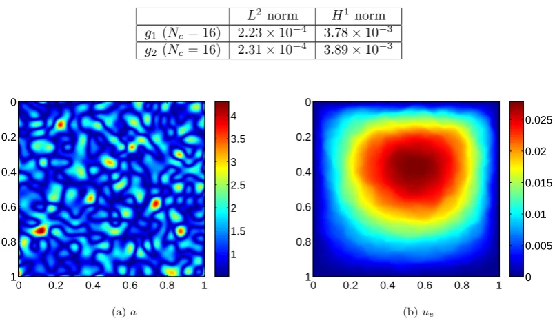
L2norm H1 norm
g1 (Nc= 16) 2.23×10⁻⁴ 3.78×10⁻³ g2 (Nc= 16) 2.31×10⁻⁴ 3.89×10⁻³
0 0.2 0.4 0.6 0.8 1
0 0.2 0.4 0.6 0.8 1 1 1.5 2 2.5 3 3.5 4 (a)a
0 0.2 0.4 0.6 0.8 1
0 0.2 0.4 0.6 0.8 1 0 0.005 0.01 0.015 0.02 0.025
(b)ue
Figure 2.3: Example 2.2 - The coefficientaand the exact solutionue
0 0.2 0.4 0.6 0.8 1
0 0.2 0.4 0.6 0.8 1 0.5 1 1.5 2
(a) ∂F1
∂x1 (Nc= 16)
0 0.2 0.4 0.6 0.8 1
0 0.2 0.4 0.6 0.8 1 0.7 0.8 0.9 1 1.1 1.2 1.3 1.4
(b) ∂g1
[image:42.595.125.523.370.535.2]∂x1 (Nc= 16)
Figure 2.4: Example 2.2 - The derivative of the functionF andg (Nc= 16)
Table 2.5: Example 2.2 -L2 norm relative errors of the solution
MsMRM FEM
Nc= 8 3.02×10⁻² 1.06×10⁻¹ Nc = 16 7.33×10⁻³ 6.89×10⁻² Nc = 32 3.50×10⁻³ 3.89×10⁻²
Table 2.6: Example 2.2 -H1 norm relative errors of the solution
MsMRM FEM
Table 2.7: Example 2.2 -L∞ norm of the functionχ
χ1 χ2
Nc= 8 2.42×10⁻² 2.40×10⁻² Nc = 16 1.52×10⁻² 1.36×10⁻² Nc = 32 7.20×10⁻³ 7.56×10⁻³
Table 2.8: Example 2.2 -L2 norm andH1 norm relative errors of the functiong(N
c= 16)
L2norm H1 norm
g1 (Nc= 16) 1.86×10⁻⁴ 4.02×10⁻³ g2 (Nc= 16) 2.11×10⁻⁴ 4.49×10⁻³
contrast coefficient (see Figure 2.5a). The contrast in the coefficient is as high as 105. The channel is 0.02 wide in bothx and y directions, and 0.5 long inx direction and 0.3 long in y direction. Inside the channel, the coefficient is very large (= 105), while
the coefficient is small outside the channel (= 1). There has been a lot of interest in studying multiscale problems with high contrast coefficients in recent years, see e.g. [18, 23, 22, 31]. This is known to be a very difficult problem. In this example,
f(x, y) = sin(0.33πx+ 0.43) cos(0.43πy + 0.38). Even for such a challenging test problem, our method still captures the important feature of the solution accurately. As we can see from Table 2.9-2.10, the convergence rate remains to be very robust and the relative errors are very small.
0 0.2 0.4 0.6 0.8 1
0
0.2
0.4
0.6
0.8
1
2 4 6 8 10 x 104
(a)a
0 0.2 0.4 0.6 0.8 1
0
0.2
0.4
0.6
0.8
1
1 2 3 4 5 x 10⁻³
[image:43.595.121.531.457.629.2](b)ue
0 0.2 0.4 0.6 0.8 1 0
0.2
0.4
0.6
0.8
1
0 1 2 3 4 5 6
(a) ∂F1
∂x1 (Nc= 16)
0 0.2 0.4 0.6 0.8 1
0
0.2
0.4
0.6
0.8
1
0.5 1 1.5 2 2.5 3
(b) ∂g1
[image:44.595.127.523.99.269.2]∂x1 (Nc= 16)
Figure 2.6: Example 2.3 - The derivative of the functionF andg (Nc= 16)
Table 2.9: Example 2.3 -L2 norm relative errors of the solution
MsMRM FEM
[image:44.595.232.409.452.505.2]Nc= 8 3.88×10⁻² 1.30×10⁻¹ Nc = 16 9.06×10⁻³ 8.84×10⁻² Nc = 32 3.99×10⁻³ 3.59×10⁻²
Table 2.10: Example 2.3 -H1norm relative errors of the solution
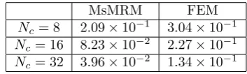
MsMRM FEM
[image:44.595.237.408.559.610.2]Nc= 8 2.09×10⁻¹ 3.04×10⁻¹ Nc = 16 8.23×10⁻² 2.27×10⁻¹ Nc = 32 3.96×10⁻² 1.34×10⁻¹
Table 2.11: Example 2.3 -L∞norm of the function χ
χ1 χ2
Nc= 8 1.63×10⁻¹ 1.18×10⁻¹ Nc = 16 7.26×10⁻² 6.58×10⁻² Nc = 32 5.80×10⁻² 3.64×10⁻²
Table 2.12: Example 2.3 -L2 norm andH1norm relative errors of the functiong (N
c= 16)
L2norm H1 norm
Example 2.4. We consider the elliptic PDE with the following coefficient
a(x, y) = exp
10
X
i=1
wi(αisin(2πx/wi) +βicos(2πx/wi))
!
,
where αi and βi are independent uniform random variables in [− √
3,√3], and (w1, ..., w10) = 12,13,15,17,111 ,131 ,171,191,231,291
. As we can see from Figure 2.7a, the coefficient varies rapidly inxdirection, and it has many layers, which makes the prob-lem very difficult to solve. In this example,f(x, y) = sin(0.44πx+ 0.46) cos(0.28πy+ 0.26). For such a problem, our method works very well and captures the small scales inx direction. As we can see from Table 2.13-2.14, the relative errors are very small. We also note that there is no variation in y direction, so the norm of χ2 and the
numerical errors for g2 are 0, as expected (Table 2.15-2.16).
0 0.2 0.4 0.6 0.8 1
0
0.2
0.4
0.6
0.8
1
0.5 1 1.5 2 2.5
(a)a
0 0.2 0.4 0.6 0.8 1
0
0.2
0.4
0.6
0.8
1 0
0.01 0.02 0.03 0.04 0.05
(b)ue
Figure 2.7: Example 2.4 - The coefficientaand the exact solutionue
Table 2.13: Example 2.4 -L2 norm relative errors of the solution
MsMRM FEM
Nc= 8 2.43×10⁻² 1.35×10⁻¹ Nc = 16 7.29×10⁻³ 4.91×10⁻² Nc = 32 3.03×10⁻³ 1.18×10⁻²
0 0.2 0.4 0.6 0.8 1 0
0.2
0.4
0.6
0.8
1
0.5 1 1.5 2 2.5
(a) ∂F1
∂x1 (Nc= 16)
0 0.2 0.4 0.6 0.8 1
0
0.2
0.4
0.6
0.8
1
0.5 1 1.5 2
(b) ∂g1
∂x1 (Nc= 16)
Figure 2.8: Example 2.4 - The derivative of the functionF andg (Nc= 16)
Table 2.14: Example 2.4 -H1norm relative errors of the solution
MsMRM FEM
Nc= 8 1.95×10⁻¹ 3.90×10⁻¹ Nc = 16 9.22×10⁻² 2.36×10⁻¹ Nc = 32 4.15×10⁻² 1.01×10⁻¹
Table 2.15: Example 2.4 -L∞norm of the function χ
χ1 χ2
Nc= 8 3.95×10⁻² 0 Nc= 16 2.17×10⁻² 0 Nc= 32 6.74×10⁻³ 0
Table 2.16: Example 2.4 -L2 norm andH1norm relative errors of the functiong (N
c= 16)
L2norm H1 norm
in many regions. In this example, f(x, y) = sin(0.35πx+ 0.23) cos(0.21πy+ 0.06). As we can see from Table 2.17-2.18, our method still provides satisfactory results and the errors are small, which shows that our method can be used to solve challenging multiscale problems without scale separation and with discontinuous coefficients.
0 0.2 0.4 0.6 0.8 1
0 0.2 0.4 0.6 0.8 1 10 20 30 40 50 (a)a
0 0.2 0.4 0.6 0.8 1
0 0.2 0.4 0.6 0.8 1 0 0.005 0.01 0.015 0.02
(b)ue
Figure 2.9: Example 2.5 - The coefficientaand the exact solutionue
0 0.2 0.4 0.6 0.8 1
0 0.2 0.4 0.6 0.8 1 1 2 3 4 5 6 7
(a) ∂F1
∂x1 (Nc= 16)
0 0.2 0.4 0.6 0.8 1
0 0.2 0.4 0.6 0.8 1 1 2 3 4 5
(b) ∂g1
∂x1 (Nc= 16)
Table 2.17: Example 2.5 -L2 norm relative errors of the solution
MsMRM FEM
Nc= 8 7.29×10⁻² 9.84×10⁻¹ Nc = 16 3.68×10⁻² 3.74×10⁻¹ Nc = 32 1.12×10⁻² 1.70×10⁻¹
Table 2.18: Example 2.5 -H1norm relative errors of the solution
MsMRM FEM
Nc= 8 1.78×10⁻¹ 9.90×10⁻¹ Nc = 16 9.16×10⁻² 5.38×10⁻¹ Nc = 32 6.28×10⁻² 3.56×10⁻¹
Table 2.19: Example 2.5 -L∞norm of the function χ
χ1 χ2
Nc= 8 2.11×10⁻¹ 6.44×10⁻² Nc = 16 1.14×10⁻¹ 3.46×10⁻² Nc = 32 8.68×10⁻² 2.19×10⁻²
Table 2.20: Example 2.5 -L2 norm andH1norm relative errors of the functiong (Nc= 16)
L2norm H1 norm
Chapter 3
Multiscale model reduction
method for time-dependent PDEs
3.1
Effective equations
We could apply a similar idea to derive effective equations for time-dependent equa-tions with time-independent coefficients.
3.1.1 Parabolic equation
We first consider a parabolic equation of the form
ut(x, t)− ∇ ·(a(x)∇u(x, t)) =f(x), x∈D, t∈(0, T],
u(x, t) = 0, x∈∂D, t∈(0, T],
u(x,0) = 0, x∈D.
(3.1)
We can define the harmonic coordinates F in exactly the same way as we did for the elliptic equation. We then decompose F = g +χ and solve the following effective equation on a coarse mesh
(u0)t(x, t)− ∇ ·(a(x)(I+∂χ∂x∂x∂g)∇u0(x, t)) = f(x), x∈D, t∈(0, T],
u0(x, t) = 0, x∈∂D, t∈(0, T],
u0(x,0) = 0, x∈D.
(3.2)
3.1.2 Convection-diffusion equation
Next, we consider the convection-diffusion equation with multiscale velocity field (see also [47])
vt(x, t) +u(x)· ∇v(x, t) =∇ ·(α∇v(x, t)) x∈D, t∈(0, T],
v(x, t) = 0, x∈∂D, t∈(0, T],
v(x,0) = φ(x), x∈D,
(3.3)
where u(x) is a velocity field that satisfies ∇ ·u(x) = 0 and α is a positive diffusion constant.
We define the corresponding harmonic coordinates as follows
u(x)· ∇Fk(x) =∇ ·(α∇Fk(x)), x∈D
Fk(x) =xk, x∈∂D.
(3.4)
By decomposing F =g+χas before, we obtain the following effective equation
(v0)t(x, t) +u(x)· ∇v0(x, t) =∇ ·((α∂F∂x −uχT)∂x∂g∇v0(x, t)), x∈D, t∈(0, T],
or equivalently
(v0)t= n
P
i,j,k=1
(α∂F∂x −uχT) ij∂g∂xki ∂
2v0
∂gj∂gk in D×(0, T]
v0(x, t) = 0, x∈∂D, t∈(0, T],
v0(x,0) =φ(x), x∈D.
(3.5) Finally, v is approximated by v0+χT ∂x∂g∇v0.
3.1.3 Hyperbolic equation
we consider the following hyperbolic equation
utt(x, t)− ∇ ·(a(x)∇u(x, t)) =f(x), x∈D, t∈(0, T],
u= 0, x∈∂D, t∈(0, T],
u= 0, x∈D,
ut= 0, x∈D.
(3.6)
It is straightforward to generalize the derivation of our effective equation to the hy-perbolic equation. The effective equation takes the form
(u0)tt(x, t)− ∇ ·(a(x)(I+ ∂χ∂x∂x∂g)∇u0(x, t)) =f(x), x∈D, t ∈(0, T],
u0(x, t) = 0, x∈∂D, t∈(0, T],
u0(x,0) = 0, x∈D,
(u0)t(x,0) = 0, x∈D,
(3.7)
where F =g+χ is defined in the same way as before.
3.2
Error estimate
For the parabolic equation, we have the following theorem.
Theorem 3.1. Suppose u, F and u0 are weak solutions to (3.1), (2.2) and (3.2)
respectively. Let u1 =χT ∂x∂g∇u0, F =g+χ, and χ= 0 on ∂D. Then we have
max
(0,T]
ku−u0−u1kL2(D)+ku−u0−u1kL2(0,T;H1(D))
≤CkχkL∞(D)k
∂g
∂xkL∞(D)kdet( ∂x
∂g)kL∞(D)(|u˜0|H2,1(0,T;D)+k(˜u0)tkL2(0,T;H1(D))), (3.8) whereC is a constant that depends ond, Danda,u˜0(y, t) = ˜u0(g(x), t) =u0(x, t)and
kuk2
L2(0,T;H1(D)):=
RT
0
R
D(u
2+|∇u|2)dxdt,|u|2
H2,1(0,T;D) :=
RT
0
R
D((ut)
Proof. Letz =u−u0−u1, thenz = 0 at t= 0 and on ∂D. We define
p=a∇u−a∂F ∂x
∂x ∂g∇u0,
η1 =−a
∂ ∂x
∂x ∂g∇u0
χ,
η2 =−χT
∂x
∂g∇(u0)t.
Then we have
a∇z−p=a∇u−a∇u0−a∇u1−a∇u+a
∂F ∂x
∂x ∂g∇u0
=−a∇u0−a∇u1+a
∂F ∂x
∂x ∂g∇u0
=−a ∂ ∂x
∂x ∂g∇u0
χ=η1,
and
∇ ·p= (ut−f)−((u0)t−f) = ut−(u0)t=zt+ (u1)t=zt−η2.
Then for any τ ∈(0, T] we have
Z τ
0
Z
D
∇z·a∇zdxdt
=
Z τ
0
Z
D
∇z·(a∇z−p)dxdt+
Z τ
0
Z
D
∇z·pdxdt
=
Z τ
0
Z
D
∇z·η1dxdt−
Z τ
0
Z
D
z(∇ ·p)dxdt
=
Z τ
0
Z
D
∇z·η1dxdt−
Z τ
0
Z
D
(zzt−zη2)dxdt
=
Z τ
0
Z
D
∇z·η1dxdt−
Z
D
z2(τ, x)
2 −
z2(0, x)
2
dx+
Z τ
0
Z
D
zη2dxdt
=
Z τ
0
Z
D
∇z·η1dxdt−
1 2
Z
D
z2(τ, x)dx+
Z τ
0
Z
D
Rearranging the above equation, we get
1 2
Z
D
z2(τ, x)dx+
Z τ
0
Z
D
∇z·a∇zdxdt
=
Z τ
0
Z
D
∇z·η1dxdt+
Z τ
0
Z
D
zη2dxdt
≤
Z τ
0
Z
D
|∇z·η1|dxdt+
Z τ
0
Z
D
|zη2|dxdt
≤
Z T
0
Z
D
|∇z·η1|dxdt+
Z T
0
Z
D
|zη2|dxdt.
Taking the maximum over τ ∈(0, T], we have
max
(0,T]
1 2
Z
D
z2(τ, x)dx+
Z T
0
Z
D
∇z·a∇zdxdt
≤
Z T
0
Z
D
|∇z·η1|dxdt+
Z T
0
Z
D
|zη2|dxdt
≤k∇zkL2(0,T;D)kη1kL2(0,T;D)+kzkL2(0,T;D)kη2kL2(0,T;D).
where the second inequality is due to the H¨older’s inequality. Application of the Poincar´e’s inequality gives
max
(0,T]kzkL
2(D)+kzkL2(0,T;H1(D