Image Compression Using Neural Networks

San Jose State University

SJSU ScholarWorks

Master's Projects Master's Theses and Graduate Research

Spring 5-9-2019

Image Compression Using Neural Networks

Kunal Rajan Deshmukh

San Jose State University

Follow this and additional works at:https://scholarworks.sjsu.edu/etd_projects

Part of theArtificial Intelligence and Robotics Commons

This Master's Project is brought to you for free and open access by the Master's Theses and Graduate Research at SJSU ScholarWorks. It has been accepted for inclusion in Master's Projects by an authorized administrator of SJSU ScholarWorks. For more information, please contact

Recommended Citation

Deshmukh, Kunal Rajan, "Image Compression Using Neural Networks" (2019).Master's Projects. 666. DOI: https://doi.org/10.31979/etd.h8mt-65ct

Image compression using Neural Networks

A Project Presented to

The Faculty of the Department of Computer Science San José State University

In Partial Fulfillment

of the Requirements for the Degree Master of Science

by

Kunal Rajan Deshmukh May 2019

© 2019

Kunal Rajan Deshmukh ALL RIGHTS RESERVED

The Designated Project Committee Approves the Project Titled Image compression using Neural Networks

by

Kunal Rajan Deshmukh

APPROVED FOR THE DEPARTMENT OF COMPUTER SCIENCE SAN JOSÉ STATE UNIVERSITY

May 2019

Dr. Chris Pollett Department of Computer Science Dr. Nada Attar Department of Computer Science Dr. Robert Chun Department of Computer Science

ABSTRACT

Image compression using Neural Networks by Kunal Rajan Deshmukh

Image compression is a well-studied field of Computer Vision. Recently, many neural network based architectures have been proposed for image compression as well as enhancement. These networks are also put to use by frameworks such as end-to-end image compression.

In this project, we have explored the improvements that can be made over this framework to achieve better benchmarks in compressing images. Generative Adversarial Networks are used to generate new fake images which are very similar to original images. Single Image Super-Resolution Generative Adversarial Networks (SI-SRGAN) can be employed to improve image quality.

Our proposed architecture can be divided into four parts : image compression module, arithmetic encoder, arithmetic decoder, image reconstruction module. This ar-chitecture is evaluated based on compression rate and the closeness of the reconstructed image to the original image.

Structural similarity metrics and peak signal to noise ratio are used to evaluate the image quality. We have also measured the net reduction in file size after compression and compared it with other lossy image compression techniques. We have achieved better results in terms of these metrics compared to legacy and newly proposed image compression algorithms. In particular, an average PSNR of 28.48 and SSIM value of 0.86 is achieved as compared to 28.45 PSNR and 0.81 SSIM value in end to end image compression framework [1].

Keywords - Convolutional Neural Networks, Generative Adversarial Net-works, Structural Similarity Metrics, Peak Signal to Noise Ratio.

ACKNOWLEDGMENTS

I would like to express my special gratitude to Dr. Chris Pollett for his guidance for this project. Without his constant encouragement, this would not be possible.

I am also thankful to my committee members, Dr. Robert Chun and Dr. Nada Attar for providing valuable guidance.

Finally, I would like to thank my friends and family for their love and support during this time.

TABLE OF CONTENTS CHAPTER 1 Introduction . . . 1 1.1 Problem Statement . . . 1 1.2 Overview . . . 3 2 Background . . . 4

2.1 Use of Convolution Neural Networks in Image Compression . . . . 6

2.2 Use of Generative Adversarial Networks in Image Compression . . 8

2.3 Use of Recurrent Neural Networks in Image Compression . . . . 10

3 Tools and Techniques . . . 11

3.1 Convolutional Neural Networks . . . 11

3.2 Generative Adversarial Networks . . . 13

3.3 Image Quality Metrics . . . 13

3.3.1 Mean Square Error (MSE) . . . 13

3.3.2 Peak Signal to Noise Ratio (PSNR) . . . 14

3.3.3 Structural Similarity Index (SSIM) . . . 14

3.4 Dataset augmentation . . . 14 3.5 PyTorch . . . 15 3.6 Ray - Tune . . . 16 3.7 Residual learning . . . 16 3.8 Optimizers . . . 17 3.9 Dataset . . . 18

4 Network Design . . . 20

4.1 Arithmetic coder and decoder . . . 20

4.2 Image compression module . . . 20

4.3 Image reconstruction module . . . 23

4.4 Loss function . . . 26 4.5 Training . . . 27 5 Experiments . . . 28 6 Conclusion . . . 34 6.1 Future Scope . . . 35 LIST OF REFERENCES . . . 37

LIST OF TABLES

1 Results obtained on baseline model . . . 28 2 Visualization of results on baseline model . . . 29 3 Results obtained on proposed model for color images . . . 29 4 Visualization of results on proposed model for color images . . . . 30 5 Results obtained on proposed model for grayscale images . . . 30 6 Visualization of results on proposed model for grayscale images . 30

LIST OF FIGURES

1 End to end image compression framework using CNN. . . 7

2 Photo realistic Single Image Super resolution using GANs. . . 9

3 Alexnet architecture [2]. . . 11

4 Alexnet architecture. . . 17

5 Image Compression Module. . . 22

6 Image reconstruction module. . . 24

7 Image file sized before and after compression . . . 32

CHAPTER 1 Introduction 1.1 Problem Statement

Image compression is a kind of data compression. Research in data compression is at least four decades old. The Lempel-Ziv data compression algorithm as well as Differential Pulse-Code Modulation were developed in the 1970s. A modification of this algorithm : Lempel-Ziv-Welch (LZW) was published by Welch in the year 1984. This algorithm is still used in GIF image formats.

Many techniques such as Run-Length Encoding (RLE), Discrete Cosine Transform (DCT), etc. are used traditionally for image compression. These deterministic image compression algorithms rely mainly on image filters, discrete transformations and quantization. Because of Moore’s law, handheld devices and personal computers now have much higher processing power than they had at any time in the past. This has allowed the development of modern image compression algorithms. Many image compression frameworks have now been proposed, based on deep neural networks.

Several recently published articles on image processing frameworks used deep learning networks. We used parts and ideas from several of those frameworks to develop a new architecture. The goal of this project was to develop a new deep neural network architecture which is an improvement upon existing architectures in terms of efficiency and image quality metrics such as SSIM, PSNR. We also wanted to do this in most time efficient manner possible.

Jiang, et al. considered an end to end image compression network [1] in which fully convolutional neural network based encoder is used for image compression. Our proposed architecture closely follows this model. Hence on several instances,we have used this architecture as out baseline model and we have compared our performance with this architecture. In this architecture, a smaller image is constructed by encoder.

This image is nothing but a smaller replica of the original image. The decoder, in this instance called re-constructor, is designed to generate an original image back from its smaller replica. In our own implementation, average PSNR and SSIM metrics obtained were 28 and 0.56 respectively. We achieved better results than this model. Another convolutional neural network based architecture proposed by Cavigelli, et al. [3] is efficient is suppressing the artifacts which are introduced during image compression process. This architectures makes efficient use of several skip connections to train the model. We have used skip connections in our model to train our model faster.

Space separable operations such as pointwise and depthwise operations are useful to speedup training and inference process even further. We used such operations at some levels of our neural network. This has reduced the training as well as inference time required to train our model.

We have also designed a loss function such a way that image generated from compression module has a very low variance in pixel values. This limits the pixel values the resultant compresses image can have. The arithmetic encoder is used to process this compressed image. Since the compressed image now has a very small number of distinct values, an arithmetic encoder can use lossless data compression algorithms such as entropy coding or RLE to further compress the results obtained from compression module.

Hyper-parameter optimization was performed on this network to calculate hyper-parameters such as number or layers, learning rate, coefficients for loss function etc. We used hyperband scheduler for this purpose. We could improve our results using values obtained hyper-parameter search.

1.2 Overview

This report is organized as follows: The next chapter explores work related to legacy image compression algorithms and deep neural network based frameworks. In the following chapter, data augmentation techniques that are used, The motive behind using PyTorch framework and some useful API, a library used for hyper-parameter optimization, concepts such as residual learning and datasets we explored as a part of this project are explained. The report later explains a new proposed architecture and experiments carried out on it. We conclude this report with achievements and future work.

CHAPTER 2 Background

Image compression is necessary so as to enable saving large amounts of images in a limited storage area. Most images captured today are for human consumption. Human vision is sensitive towards some features of an image. e.g. Low-frequency components of an image are easily noticed while high-frequency components are not. This fact is used in lossy image compression algorithms. Hence, lossy image compression algorithms focus on the removal of such features from the image. In this project, our aim was to propose a new lossy image compression framework which could provide better image compression ratio while maintaining the quality of the images. In this chapter, we will explore some legacy image compression techniques along with some recently proposed architectures. Our architecture which is proposed in the fourth chapter is motivated by these existing architectures.

The recently developed algorithms like WebP and High-Efficiency Image File Format (HEIF) [4, 5] use more complex encoding structures. Even though these com-pression techniques require more computation power than the traditional algorithms like JPEG, its use results in much smaller file size while maintaining a similar quality of an image.

Before the advent of Deep Neural Networks, techniques such as Run-length encoding, Entropy encoding, Differential Pulse-Code Modulation (DPCM) were used for image compression. In run-length encoding series of bits of 0s and 1s are replaced by a bit symbol followed by a count of the number of bits. Entropy encoding method on the other hand work on a higher level of image representation. In this technique, quantized pixel values are replaced by symbols. Length of these symbols is determined on the basis of frequency of occurrence. Huffman Coding, Arithmetic Coding, and Range Coding techniques are some examples of entropy encoding techniques.

Run-length encoding and Entropy encoding techniques are lossless data compression techniques. Data is lost when quantization results in the lower granularity of values. However, it is necessary to convert analog values to its corresponding digital values. Differential Pulse-Code Modulation [6] (DPCM) is another technique used to convert an analog signal into a digital signal. In this technique, the difference between sampled values from the analog signal and predicted values is quantized and encoded. Since pixel values are predicted based on previous values, the compression factor of DPCM is higher than quantization techniques.

An Image in WebP [4] format is represented by 32 bit format. In this format, alpha channel is added along with ’R’, ’G’, ’B’ values which represent the opacity value. Lossy WebP architecture uses predictive encoding technique in which, the value of a pixel is predicted using the value of neighboring pixels. Lossless WebP compression technique uses a variety of lossless transformation techniques such as color de-correlation transform, Subtract Green Transform and color cache encoding in order to provide better lossless performance than earlier techniques. HEIF is a video and single image compression format in which images are stored in the form of thumbnails in several containers and the final image is built using those representations. HEIF format supports 16-bit color as opposed to an 8-bit color used by JPEG. HEIF format supports block sizes of 8×8to 16×16 pixels. Pixel value in each block is predicted

using the data in another block. This format uses Context-Adaptive Binary Arithmetic Coding (CABAC) [7] techniques instead of Huffman coding which is used in other popular image file formats such as JPEG. PSNR of CABAC is better than Huffman coding. In HEIF quantization parameters are decided locally and hence, it preserves both high as well as low-frequency components in an image.

Use of Neural Network in Image Compression is a relatively new development. Due to the stochastic nature of Neural Network training, the Neural Network architectures

used in Image compression are inherently lossy in nature. Generative Adversarial Networks (GANs), Convolutional Neural Networks (CNNs) and Recurrent Neural Networks (RNNs) are being used for image compression purpose.

Recently published Neural Network architectures [8, 1, 9, 10] demonstrate that, apart from tasks such as Classification, Object Detection, and segmentation; Deep Neural Networks can be employed for image compression tasks. However, these neural networks can be optimized further not only for faster image compression and retrieval times but also for better accuracy.

Various methods for weight initialization and optimizer function have been proposed for computer vision related tasks. Even though random normal weight initialization and Gradient Descent based optimization function work in many cases other methods are being proposed for faster and better convergence in the training phase. We will discuss these techniques in more detail in subsequent chapters of this report.

2.1 Use of Convolution Neural Networks in Image Compression

Our proposed architecture relies heavily on CNNs to capture image artifacts. They have been used recently in many image compression architectures.

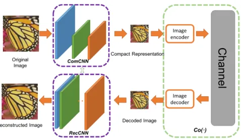
Jiang, et al. [1] has used fully convolutional auto-encoder to obtain a compressed representation of an image. The architecture shown in Figure 1 below, has two distinct parts - ComCNN and RecCNN. Series of convolutional layers stacked in this way can capture features of an image. The author claims that because of the use of multi-layer CNNs, this architecture can maintain the structural composition of an image as well. The ComCNN is a network responsible in compressing these images in such a way that resultant images can be effectively reconstructed by reconstruction network. This

Figure 1: End to end image compression framework using CNN.

network consists of three convolutional layers with the second layer followed by batch normalization layer. Since the first convolutional layer uses a stride of two, the image size is reduced by half. RecCNN layer uses twenty Neural network layers. Apart from the first and the last layer, each layer in this formation carries out Convolutional and batch normalization operation. The author trained this network using 400 grayscale images and 50 epochs. SSIM and PSNR metrics of these images are better than JPEG images.

In lossy image compression techniques, artifacts of image compression algorithm are visible in images. An example of such artifacts is visible on images for which tiling was used for quantization. In such images, these tile boundaries continue to remain in the images. CNN based architecture [3] proposed by Cavigelli, et al. is a twelve layer image compression architecture used for image compression artifact suppression. This paper not only proposes a new architecture to suppress these compression artifacts, but it also proposes a new way to train deep neural network models which is adaptable to other low-level computer vision tasks. In this paper, Cavigelli, et al. proposed hierarchical skip connections and multiscale loss functions. These

hierarchical skip connections provide two advantages - In forward pass, this method provides information to obtain higher resolution images. In backward pass, these skip connections allow gradient flow to skip middle layers and help train early layers. Even after using skip connections in deep neural networks, it still does not eliminate the possibility of very long paths. Hence, loss is calculated on many intermediate low-resolution images. The author has observed that batch normalization does not re-duce the accuracy of the network; moreover, it adds batch-to-batch jitter in the system.

2.2 Use of Generative Adversarial Networks in Image Compression Generative Adversarial Networks (GANs) are useful for tasks such as image enhancement. GANs are trained to imitate original distribution. This property is useful in image compression problem since GANs can be used for tasks such as de-blurring, to provide a better alternative for interpolation. We have used photo-realistic Single Image Super-Resolution Generative Adversarial Network (SRGAN) to perform up-scaling task in the proposed framework.

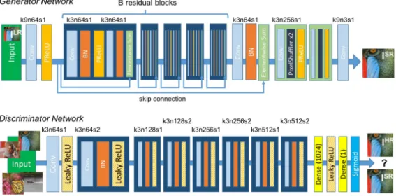
Ledig, et al. [9] explained how GANs can be used to recover finer detail about the image when it is lost because of compression. The framework proposes perceptual loss function which is made up of content loss and adversarial loss. We have used this architecture as an efficient way of image up-scaling.

This architecture up-scales the images by 4 times. Mean-Opinion-Score (MOS) of images generated using this method is close to the MOS of original images. It uses the VGG network as a Discriminator. In this paper, the author claimed that deeper neural network architectures are difficult to train and hence batch normalization layer is useful to offset co-variate shift. In a generator network, Ledig, et al. used the block layout with two convolutional layers in each block. They used parametric relu

Figure 2: Photo realistic Single Image Super resolution using GANs.

as an activation function to avoid the use of max-pooling layer in the network. In VGG, strided convolution is used to reduce image resolution as the number of kernel increases with each layer. This network was trained on 350 thousand images from ImageNet dataset.

In an other GAN based network [10] for image enhancement, instead of using perceptual loss function, Cheng, et al. used a non-parametric Bayesian model. In this model, a Dirichlet process and Gaussian process are applied in patches of a low-resolution image to obtain a high-resolution image. Markov Chain Monte Carlo (MCMC) algorithm was used for hyper-parameter optimization. Markov Chain was calculated using by sampling posterior distributions for each hyperparameter. This process is known as Gibbs sampling. This proposed method performs better than the Sparse Coding and Gaussian Process Regression Model. However, PSNR and SSIM values obtained using this process are lesser than those obtained using the earlier method. The average PSNR and SSIM matrices obtained from this method are 29.5dB and 0.843 respectively.

2.3 Use of Recurrent Neural Networks in Image Compression

Recurrent Neural Networks (RNNs) are typically used for sequential time series data predictions. RNNs ahve been used for image compression in an architecture [8] proposed by Toderici, et al. This architecture was developed small network bandwidth for handheld devices. In this architecture, the output image is refined and improved successively as more data is obtained from the network. This network consists of Encoder, Decoder, and Binizer. Long Short Term Memory (LSTM) cells are used along with convolutional layer. In each iteration of this network, an input image is encoded in encoder and binzer, as the name suggests, transforms it to a binary file. This binary file can be transferred over the network. The decoder can generate original image from this binary file. Even though this network performs better compared Vanilla CNN based approaches, every iteration of a network requires a minimum of eleven layers of RNN convolutional layers and hence, it can be a more complicated model to train. This model is more useful in the instances where compressed image data is received while image is being constructed. Since this model might have required much more processing power than available with us we decided to not to use this network.

CHAPTER 3 Tools and Techniques

This section explains various concepts and implementation details used in project implementation.

3.1 Convolutional Neural Networks

Convolutional Neural Networks [11] are primarily used for a grid-like data. This often involves image as well as other data arranged in a grid-like shape. In CNNs, each kernel results in a new convoluted layer. These layers are also called activation maps. As the name suggests, in this network, the convolution operation is used instead of matrix multiplication. As shown in Figure 3, In this operation, a kernel or a mask moves over an image and a convoluted representation is calculated as an output. CNNs can capture special and temporal dependencies in an image. This property

Figure 3: Alexnet architecture [2].

is extremely useful in computer vision tasks such as Image classification and image classification. In an image classification [2, 12, 13, 14] networks, series of convolution layers are followed by fully connected layers which help in classification. Depth of Convolutional Neural Networks decides how nuanced the observations of a network can be. Lower layers of CNNs are responsible for lower level features such as line, corners, etc. while higher level layers are responsible for more higher level features.

Size of intermediate results can be reduced by using stride. Stride is an offset by which kernels are moved during convolution operation.

Point-wise Convolutional Neural Networks

Point-wise convolutional operation is a type of special operation where the size of the kernel is always 1×1. This operation returns a layer with the same dimensions

as that of input layers.

Depthwise Convolutional Neural Networks

As the names suggest, Depthwise CNNs work on depth. Each kernel can have any height and width, however, its depth is always one. Separate kernels act on each depth level. Stacking all these layers together results in an image.

Point-wise and Depth-wise convolutions involve much fewer multiplications. This can be proved by a simple calculation [15] - let us assume there are 16 kernels in total. Let us assume the kernel size is 5x5x3 and we move it 8 times for both length and breadth.

Hence the total multiplications required are : 16·3·5·5·8·8 = 76800

If we decide to use depthwise and pointwise convolution instead then

For depthwise convolution, we will have three kernels instead of one. Hence the calculation will be - 3·5·5·8·8 = 4800

For pointwise convolution we got 16·1·1·3·8·8 = 3072

Hence, the number of multiplications required is 4800 + 3072 = 7872

This is much less than multiplications required for normal convolution layers. Since space separable convolutions results in less number of parameters than the normal CNNs, shallow neural networks with space separable convolutions may fail to learn during training.

3.2 Generative Adversarial Networks

Generative Adversarial Networks (GANs) are the improvement over Generative Networks. GANs consists of 2 networks that are pitted against each other in order to achieve better results in both sections. The generative network is responsible for generating fake data as close to the original data as possible and discriminative network is an image classification algorithm which discriminates fake images from original images. Trained GANs are well-trained networks which closely mimics real-world data.

3.3 Image Quality Metrics

Image quality metrics are useful for us to measure how well an architecture has performed. These can also be used to define loss in neural networks. Image quality metrics are of two types : reference image quality metrics and non-reference image quality metrics. Non-reference image quality metrics like Mean Subtracted Contrast Normalized (MSCN) do not require a reference image to compare an image with.

Since we are going to compare the uncompressed image with the original image in this project, we have used only reference image quality metrics. Here, we will review some reference image quality metrics.

3.3.1 Mean Square Error (MSE)

MSE calculates the addition of squared differences between pixel values of two images. 𝑀 𝑆𝐸 = 1 𝑀 𝑁 𝑀 ∑︁ 𝑦=1 𝑁 ∑︁ 𝑥=1 [𝐼(𝑥, 𝑦)−𝐼′(𝑥, 𝑦)]2

Here, M and N is a size of image1 and image2 respectively. I(x,y) is a pixel value at position x,y. This is the simplest image quality metric to understand. However, This metric is not always a good metric to access image compression quality since it

does not take into account the range of variations in pixel values in an image and high, low-frequency components in an image. These factors, however, affect human perception towards quality.

3.3.2 Peak Signal to Noise Ratio (PSNR)

PSNR is a measure of peak error between two images. This method is used to calculate the quality of compression method where higher PSNR value represents better quality of compression of an image.

𝑃 𝑆𝑁 𝑅= 10 log₁₀ 𝑅

2 𝑀 𝑆𝐸

where R represents maximum fluctuation in input image pixel values.

3.3.3 Structural Similarity Index (SSIM)

SSIM calculates quality degradation in an image due to image processing tasks such as compression. SSIM is considered a better metric to access degrada-tion of images because it takes into account visible structures of an image. SSIM is calculated using a combination of variance and covariance terms between two images.

3.4 Dataset augmentation

Data augmentation is used introduced to regularization in deep neural networks. Augmentation in images increases the effective dataset size and hence helps the neural network learn important features about images. We applied data augmentation techniques such as random cropping, random scaling, random flips and rotation of images and random changes in colors of an image.

3.5 PyTorch

PyTorch, TensorFlow and Caffe are some of the most popular deep learning frameworks. We have used PyTorch framework to design a deep neural net framework for the following reasons :

• PyTorch methods interact natively with Python source code.

• The execution workflow of PyTorch can be altered with native python statements and hence, tensor values can be accessed at the time of script execution by python statement.

• PyTorch is compatible with TorchVision - a rich API for computer vision tasks such as a module to load images into a dataset, data augmentation, etc. • PyToch has online support second only to TensorFlow.

• Native Python operations such as addition, subtraction can be used with tensors on PyTorch. That is to implement skip connections, users can simply add a tensor from the previous step to the current output.

• The documentation available for anyone to get started with PyTorch is com-prehensive and easy to understand. Starter code provided by the framework ensures programmers don’t face a steep learning curve.

We used TorchVision API provided by pytorch for data load and data augmentation operations. torch.nn API provides many useful high-level functions such as conv2d to construction 2d convolution layer, BatchNorm2d function provides an easy API to implement batch normalization layer. torch.nn API also provides functions such as relu to implement non-linear activation functions and MSELoss to implement mean squared error loss function. optim API pro-vides various optimizers such as Adam optimizer, stochastic gradient descent optimizer.

3.6 Ray - Tune

The ray library in Python is useful in the development of parallel execution framework. We used Tune API of ray library to perform hyperparameter tuning. This API supports schedulers such as Hyperband scheduler, Median Stopping Rule, Population-Based Training, etc. We have used a grid search to generate hyper-parameter values.

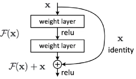
3.7 Residual learning

In the human brain, neurons do not always connect with each other in a sequential manner. A residual neural network (resnet) [13] is the network designed that is designed to mimic biological neurons. It uses skip connections in order to improve efficiency of the learning process.

Residual learning is achieved using skip connection between multiple layers. In residual learning, as shown in Fig. 4 non-linearity is applied after skip connections. Skip connections were first introduced by Long et al [16]. They are highly used in very deep neural networks such as resnet. Much deeper neural networks suffer from the problem of degradation of the gradient. The backpropagation, thus, cannot train a very long sequential deep model. This results in higher training error for the model even if the problem is not overfitted to the training data. Instead of hoping that layers will fit the underlying distribution, it is easier to train the neural network with skip connections. If a function can be trained by a deep neural network with nonlinear layers, it can also be approximated using residual connections. Any deep neural network can be approximated by its shallow version, added skip connections add the layers with identity mapping which moves the weights of multiple nonlinear mapping towards identity function. Even though identity mapping is unlikely to be

Figure 4: Alexnet architecture.

an underlying function, it is useful to bring the network closer to identity mapping than the zero mappings.

3.8 Optimizers

The 𝑡𝑜𝑟𝑐ℎ.𝑜𝑝𝑡𝑖𝑚 package provides an Adam optimizer, a RMSprop optimizer

and a Stochastic Gradient Descent (SGD) optimizer. SGD is a variant of the gradient descent optimizer. We only considered SGD and Adam optimizer in this project. The SGD optimizer works on a small subset of randomly selected data. It produces similar result to gradient descent when the learning rate is set to low. However, due to this limitations, SGD proves to be too slow for some deep learning tasks.

A recently proposed optimizer known as Adam optimizer provides faster conver-gence time.It combines the advantages of two SGD extensions : Root Mean Square Propagation (RMSProp) and Adaptive Gradient Algorithm (AdaGrad). Even though SGD optimizer sometimes provide better performance over adam, Adam is widely used in deep learning field because it provides quicker results. In this project, we tried Adam as well as SGD optimizer, however, we observed that adam provided better

performance for 50 epochs on CIFAR10 dataset.

Adam optimizer is declared in pytorch using the code as below -optim .Adam( model1 . parameters ( ) , l r =1e−3)

We used two separate optimizes for image compression as well as reconstruction part. However, both modules are trained simultaneously. With better computational resources and bigger dataset, or a dataset of narrower domain, effort can be made to use SGD optimizer in place of Adam optimizer to ensure global minima is achieved. Use of Adam optimizer has allowed us to compared performance of newly proposed network with baseline architecture.

3.9 Dataset

We explored CLIC, ImageNet, STL10, COCO and CIFAR10 datasets. CLIC

The CLIC dataset is published by Workshop and Challenge on Learned Image Com-pression. This dataset contains 1600 train images and 102 validation images. These images are high-resolution images which are a very good representation of real-world images being captured at present.

ImageNet

The ImageNet dataset contains more than 14 million images. Most modern world deep neural networks are trained on ImageNet dataset. It consists of images of random resolution and format.

CIFAR10

This dataset consists of 60K images of 32 x 32 size. Due to its image size, it can not be used to train a network for visualization. However, we have found this dataset very useful for benchmarking and for hyper-parameter optimization.

STL10

This dataset contains 100K images of 96×96 size. We have used this dataset for the

visualization of our results. COCO

This dataset is primarily used for image segmentation tasks. It consists of over 330K images. While using this dataset, we have resized all images to 200×200 size due to

CHAPTER 4 Network Design

Our proposed architecture consists of four parts - Image Compression Module (ICM), Arithmetic Encoder, Arithmetic Decoder and Image Reconstruction Module (IRM).

Out of these four modules, ICM and IRMs are used for lossy image compression while Arithmetic Encoder and Decoder deliver a lossless image compression. Both ICM as well as IRM is based on deep neural networks.

4.1 Arithmetic coder and decoder

Arithmetic coder and decoder are made up of python implementation of Huffman coding [17]. In Huffman coding, 0-255 values of pixels are treated as separate symbols, the frequency table is calculated, and this symbol is replaced by a sequence of bits. The number of bits used to represent a given symbol is inversely proportional to the frequency of that symbol. Huffman coding was implemented using reference arithmetic coding library in python. Since original data can be completely retrieved in the decoder part, it is a lossless compression algorithm and its introduction or removal does not affect other neural network-based modules.

For the purpose of neural network training, we did not use an arithmetic coder or decoder so as to avoid unnecessary computational overhead.

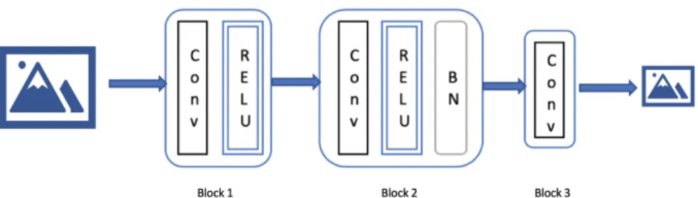
4.2 Image compression module

The image compression module consists of a series of CNN layers. These CNN layers are used to learn features of the images which can be useful for further image reconstruction tasks. Series of convolutional neural networks identify latent features in images and helps to develop series of feature maps which could hold information useful for identifying critical components in an image. These components includes

overall structure of an image as well as some salient features such as edges and corners which can not be regenerated by reconstruction layer unless they are provided as an input. Thus, this module acts as a filter though which only few critical components are passed to an intermediate image. We have performed hyper-parameter optimization on this component where we tried three, five and ten layers. However, performance of overall network did not improve with more layers in this module. Hence, we have used a three layer CNN module as shown in fig. 5 Network specification is as below:

Block 1

First Block includes a CNN layer followed by a rectified linear unit (relu) non-linearity. This CNN layer has a kernel of size 3x3 and depth as three in case of RGB image. This depth can be changed to one for the grayscale image. PyTorch reads an image in such a way that all pixel values are between zero and one. Hence, we concluded that relu function is a good fit for the data in this range. This layer is responsible for identifying low-level features in an image which are required for reconstruction framework in order to generate a realistic image.

Block 2

The second block uses a CNN layer, relu for non-linearity and a layer for batch-normalization. The CNN layer in this block uses padding values of two between the layers. This results in the tensor of half the size of the original image. We used pointwise and depthwise convolution instead of normal convolution layer in this block. This block is tasked with resizing an original image. This layer thus reduces the size and resolution of an image by half, if the stride is defined as two. Even if the image size can be reduced by interpolation techniques, the use of neural network helps in removing the information that is not useful of IRM, instead of simply re-scaling the

tensor to the desired size.

Figure 5: Image Compression Module.

We used space separable CNN layer in this block. Despite its minimal performance gain for inference task, this was preferred as its performance was better than the baseline convolutional layer. The resultant tensor is passed through batch normalization layer. This layer helps [18] avoid gradient overflow or underflow and makes the neural network less sensitive towards the choice of random initializer and its variation.

Block 3

A single convolution layer is used as the third block of the network. This layer generates the feature maps which helps the network to learn higher level features. The output of this layer is not subject to non-linearity as the goal of this layer is to reproduce an image as close to the original image as possible.

This module is trained along with reconstruction module. Hence, the goal of this network is to generate an intermediate representation of an original image, which could be used by reconstruction layer to generate an image as close to the original image as possible. Size of this intermediate result decides the compression factor of the compression algorithm. This compression factor can be changed by variation of stride and dilation values in the intermediate layer.

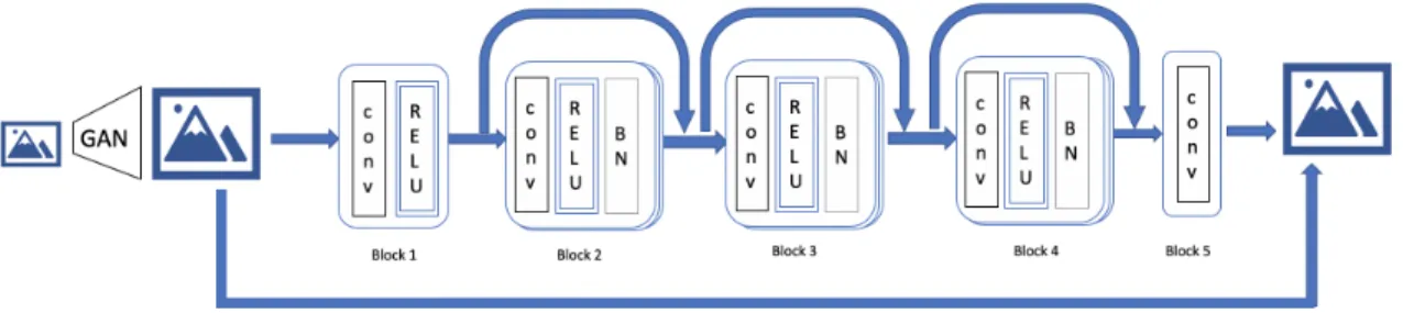
4.3 Image reconstruction module

Reconstruction module is tasked at regenerating an image such that it is very similar to the original image. The reconstruction module has on two responsibilities -Resize an image to the original size and improve the quality of the resized image.

Since this module is tasked with regeneration of an image from a minimal information passed on by compression module, this module requires more layers to hold information on how to reconstruct an image. This information is held in feature maps of convolutional layers. The first few layers are responsible in reconstruction of basic shapes such as line, points, corners etc. while further layers adds more information about the image such as facial expressions. The size of kernel used in this network is maintained at 3×3 since all these features are local to a region and are

less likely to have any impact on other parts of an image.

In end to end image compression framework[1], the author decided to use bicubic interpolation method to resize the compressed image to its original size. However, We decided to use SRGAN [9] for this purpose. This network returns the image of size four times bigger than the actual image. This image can be scaled down to the desired size using the interpolation technique before it is fed to the reconstruction module. SRGAN is known to generate an image with much better quality as compared to simple interpolation techniques. This method gives us an advantage of better input data for image enhancement. We would like to note that, while training this network, we decided to use interpolation technique for upscaling instead of GAN due to the overhead GAN might have caused during the training phase.

Moreover, this allowed us to use bad quality images to train the network for image enhancement. Slightly bad quality data is often generated as a part of data

augmentation task for robust training. Using a bicubic interpolation instead of SRGAN alleviated some need for data augmentation to training reconstruction network. SRGAN was trained separately in its original proposed shape on the ImageNet dataset. The IRM consists of five blocks each containing one convolutional layer and an optional batch normalization or relu layer.

Figure 6: Image reconstruction module. Block 1

Block one contains a CNN layer and relu layer. For this CNN layer, in channel value is the same as the number of channels. We used our channel value as 64 and3×3kernel.

Hence, this layer accepts a tensor of size Height x Width x channels and transforms it into tensor of size Height x Width x 64. Even though tensor is reshaped to this new size and original structure of pixels is lost, this shape provides more avenues for the network to add information to an image in order to produce realistic image. In other words, this resizing allows us to have more learnable weights in the following layers which could store more information about the latent characteristics of images used to train this network.

Block 2

This block is an integration of CNN, ReLU and batch normalization layers. These three layers are iterated for five times. Hence, overall, this block contains five CNN, ReLU and Batch normalization layers. A skip connection is added to short this block.

Block 3

We used pointwise and depthwise CNN layers instead of ordinary CNN layer in block 3. In all other aspects third block is similar to second block.

Block 4

This block is identical to second block. This block is added in order to improve convergence of neural network while training on rich dataset like COCO. These extra layers help in reconstruction of an image since they provide more feature maps and allows the network to learn more nuanced feature about train images.

Block 5

Fifth block consists of a CNN layer which takes 64 in channels and outputs a tensor of size Height x Width x channels.

Skip connections

After 2𝑛𝑑_,3𝑟𝑑 _{and 4}𝑡ℎ _{block, a skip connection is added as shown in fig. 6 relu is}

applied after this addition.

An interpolated image at the start of the network is added to the output of fifth block. The resultant tensor is saved as an image. As we have discussed in last chapter, skip connections are useful in backpropagation. Addition of relu also ensures that the tensors passed in the these layers are subjected to enough non-linearity and hence network weights in successive layers are not updated in the uniform manner during development. Activation functions also ensures that the resultant values in tensors are maintained in the desired domain. Since we have used batch normalization layer in the network, use of relu does not contribute to exploding gradient problem. In skip connections, two tensors of same dimension are added and each new tensor is passed through at least one convolutional layer, this ensures that convolutional layer weights are adjusted in training phase so as to accommodate the values obtained from skip connections.

4.4 Loss function

Loss function indicates the values to be minimized while training a neural network. Our loss function calculates the difference between observed output 𝑦̂︀and underlying

function y. Since this problem is a regression problem, we decided to use quadratic loss function (mean squared error) between input and output image as our loss function. In order to achieve image compression the compressed image should contain least amount of information. We used mean absolute error loss function to reduce variance in the compressed image. The image obtained from compression module ICM is compared with the reference image. mean absolute error is calculated as a difference between pixel values of a compressed image and the reference image.

Neural networks work efficiently with relu non-linearity when the values in a tensor are in the range of (0,1). Hence, we decided to use tensor with all values as 127.5 as our reference image.

Hence, our first loss function is a quadratic loss between an image provided as an input to ICM and an image received as an output from the IRM. We have defined the second loss function as the mean absolute error between a tensor with all values as 127.5 and a compressed image.

The penalty applied on a compressed image results in an image with very small variance. This fact is exploited in arithmetic encoder in order to efficiently compress the image further. Since information passed to IRM is a variance information from this image, sufficient regularization is required on this loss function to ensure that image can be reconstructed from this variance. Hence, loss obtained from using MSE between the original image and targeted image is considered as a principle loss and it is prioritized over the loss produced due to variance in compressed image. This

prioritization is achieved by dampening the loss obtained due to mean absolute error between the compressed and reference image.

4.5 Training

We have trained our neural network on STL10, CIFAR10, COCO and CLIC image datasets for varying number of epochs and network sizes.

We conclude that we got the best results with 50 epochs of COCO dataset. It required more than 110 hours of training on Google Cloud instance with Nvidia Tesla P 100 GPU. We used the image size of 200x200 for this training. As stated earlier, SRGAN and arithmetic encoder and decoders were not added to the network during training time.

CHAPTER 5 Experiments

Our first expriment made use of the baseline model [1] For this baseline model, we did not achieve the same results as claimed by the author. This could have been because we could not obtain the original dataset used by authors hence we trained our the network on publicly available datasets. We implemented the image augmentation techniques described in the paper, however, we could not train our model using only 400 images as described in the paper. We observed that network performance increased when we increased images in our datasets. This points towards the fact that image augmentation techniques we used were not sufficient to train the network using a very limited dataset. In stochastic gradient descent, weights are initialized randomly in the beginning. The choice of algorithms used to initialize these wights may affect the overall training of the model. The framework used to implement this network also contributed to challenges in reproducibility of the results for example, PyTorch loaded all images as a tensor with values between 0 and 1. Thus normalization was not required for images loaded using stand APIs in PyTorch.

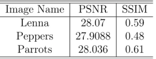
The results we obtained from implementation of the baseline model are shown in Table 1 and Table 2

Table 1: Results obtained on baseline model Image Name PSNR SSIM

Lenna 28.07 0.59

Peppers 27.9088 0.48 Parrots 28.036 0.61

Note: This result is only the grayscale images as only grayscale images were used by the authors.

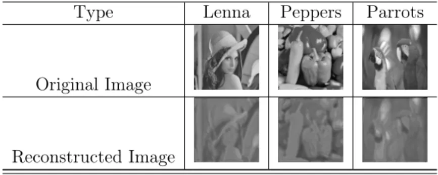
Table 2: Visualization of results on baseline model

Type Lenna Peppers Parrots

Original Image Reconstructed Image

Even though the baseline model results were obtained only on grayscale images, we could scale the model for color images as well. With the proposed method, we could obtain much better results as shown in Table 5 and Table 6. These are the results of color images.

Table 3: Results obtained on proposed model for color images Image Name PSNR SSIM

Baboon 27.7869 0.89

Lenna 29.26 0.86

Peppers 28.46 0.79 Parrots 28.33 0.69 Average 28.45 0.81

These results show some distortion in color images as IRM introduced some errors during regeneration of images. In our view, this distortion can be reduced if deeper neural network with the much bigger dataset is used to train the network. This is an error in our model. This can be reduced by using computer vision techniques outside deep learning domain such as smoothing or removal of high-frequency areas.

This architecture can be used for grayscale images as well. For this change, only the first and last layer of image compression network and image reconstruction

Table 4: Visualization of results on proposed model for color images

Type Baboon Peppers Parrots Lenna

Original Image Reconstructed Image

network needs to be changed. In this case, the number of in channels for the first CNN layer is one. The number of out channels for the last CNN layer is one.

Table 5: Results obtained on proposed model for grayscale images Image Name PSNR SSIM

Cameraman 27.34 0.78 Peppers 28.30 0.88 Lenna 29.88 0.87 Parrots 28.23 0.89 House 28.67 0.89 Average 28.48 0.86

Table 6: Visualization of results on proposed model for grayscale images

Type Cameraman Peppers Parrots Lenna

Original Image Reconstructed Image

still better than color images. The grayscale images could be more tolerant to a small error in pixel values because neural network performs better in smaller sample size and in grayscale, sample size smaller by a factor of three as compared to color images.

Grayscale images are generated using a two-dimensional tensor. Since the possibility of error is reduced by the factor of three, an error in grayscale is not easily perceived by a human eye. Since SSIM metric is modeled after human per-ception, we can see grayscale images perform better SSIM metric as compared to PSNR. The proposed algorithm is also efficient in training time (For COCO dataset): The time required to train one epoch of the baseline algorithm: 173min

The time required to train one epoch of our proposed algorithm: 137min The time required for inference:

We have measured time for inference in images per second (200×200 images).

Number of images processed every second for baseline algorithm is 4.2 whereas number of images processed per second for proposed algorithm where bicubic interpolation is used as the first stage in reconstruction phase is 4.8. When SRGAN is used, number of images per second for the proposed algorithm is 3.1

This can be construed from the fact that time required for reference is a number of arithmetic operations performed in such a task. These operations vary based on the size of a tensor, the number of layers in a neural network, size of a kernel in CNN layers. Since the framework that uses SRGAN adds more than 20 layers to the existing framework, this architecture suffers from performance degradation. However, since SRGAN can be used independently, can be applied in parallel with this architecture.

Image compression module and arithmetic encoder.

Figure 7: Image file sized before and after compression

We also analyzed the compression ratios for images of various file types. average file size and its compressed versions are as below.

Figure 8: Average file size for image file format

variety of file formats. The loss and overall quality for the image file formats do not vary substantially with the change in file formats. This is because, once an image file is read in deep learning framework, it is represented as a tensor of floating point numbers and performance of a model does is not affected based on the file format. The same was true for implementation of a baseline model as well.

CHAPTER 6 Conclusion

We implemented a baseline architecture as described by the authors in the end to end image compression framework [1]. However, due to a variety of factors described earlier chapter, the results we obtained from this implementation were inferior to the ones claimed by the authors. We used open and free datasets to perform experiments on the model and designed a new architecture with components from SRGAN[9]. The proposed network also makes use of a few newly described techniques in deep learning such as separable convolutions.

We performed experiments over the kernel size, types of layers, normalization and optimizer type. The proposed framework is a mix of SRGAN[9] and end-to-end[1] image compression network. Recurrent neural network based architecture proposed by [8] was not considered because it was overall less flexible and required more resources for training. In this architecture, we replace the bicubic interpolation layer in the original network[1] with SRGAN and we have introduced some skip connections as proposed in image compression artifact suppression network [3] to improve the performance. We also observed that point-wise and depth-wise convolution has better efficiency than CNN layer with 3x3 kernel hence we replaced some CNN layers in Compression and Reconstructor network with pointwise and depthwise convolutional layers. The resultant architecture has four components: an image compression module, Arithmetic Encoder, Arithmetic Decoder, and an image reconstruction module.

The SSIM and PSNR metrics obtained with our new framework in some cases beats recently proposed deep neural networks. The architecture also takes lesser time for the training as compared to the baseline architecture.

From our experiments, we observed that this framework not only performs better than our implementation of baseline model but also performs better than many deep

learning based frameworks proposed[1]. The architecture performs better in a smaller sample space.

The time required for the execution of deep learning framework is largely propor-tional to the number of neural network layers. Since this architecture makes use of SRGAN during image up-scaling phase, the number of layers in the model increase dramatically as compared to the baseline model. however, SRGAN can be run in parallel to the image reconstruction module in the inference phase. This can reduce the overall time required for inference for this module to a time comparable with baseline implementation.

The training time of a model can be reduced by using skip connections. These skip connections allow the gradient to flow easily to the starting layers of the network. This results in faster training of the layers at the start of the network and thus the overall network trains faster using skip connections. Performance gain at the training time along with performance boost by using point-wise and depth-wise CNN layers results in an overall efficient network as compared to the baseline network.

We also observed that this compression framework is agnostic to file format used for the compression. Even though image size varies based on the encoding used in the file format, the overall performance of the model remains unchanged.

6.1 Future Scope

In our implementation, we used Ray AI library for hyper-parameter tuning. The architecture that we proposed in this paper was the best configuration we could find in this search. However, there is always a scope to perform such a search in a bigger space. With more computational resources, hyper-parameters can be searched over much larger parameter space for the same architecture. This might result in better

performance. The literature on Batch Normalization and skip connection may develop in the future. This could be used to redesign this network.

Instead of general purpose deep learning model, an algorithm can be designed to perform in narrow domain or images such as landscape images, urban outdoor images, etc.

We observed that reconstructed gray-scale image quality is better than color images. A layer type or a network better suited for color images could be explored in the future.

New techniques and tools are being developed in deep learning for computer vision such as capsule networks. Use of such tools for image compression can be explored.

LIST OF REFERENCES

[1] F. Jiang, W. Tao, S. Liu, J. Ren, X. Guo, and D. Zhao, ‘‘An end-to-end compres-sion framework based on convolutional neural networks,’’ IEEE Transactions on

Circuits and Systems for Video Technology, vol. 28, no. 10, pp. 3007--3018, 2018.

[2] A. Krizhevsky, I. Sutskever, and G. Hinton, ‘‘Imagenet classification with deep convolutional neural networks,’’ InAdvances in neural information processing

systems, pp. 1097--1105, 2012.

[3] L. Cavigelli, P. Hager, and L. Benini, ‘‘Cas-cnn: A deep convolutional neural net-work for image compression artifact suppression,’’ International Joint Conference

on Neural Networks (IJCNN), pp. 752--759, 2017.

[4] G. Ginesu, M. Pintus, and D. D. Giusto, ‘‘Objective assessment of the webp image coding algorithm,’’ Signal Processing: Image Communication, vol. 27,

no. 8, pp. 867--874, 2012.

[5] M. Hannuksela, J. Lainema, and V. Vadakital, ‘‘The high efficiency image file format standard [standards in a nutshell],’’ IEEE Signal Processing Magazine

Magazine, vol. 32, no. 4, pp. 150--156, 2015.

[6] J. B. O. Jr., ‘‘Predictive quantizing systems (differential pulse code modulation) for the transmission of television signals,’’ https://onlinelibrary.wiley.com/doi/ abs/10.1002/j.1538-7305.1966.tb01052.x, May 1966, (Accessed on 04/21/2019). [7] I. U. Khan and M.A.Ansari, ‘‘Comparative study of huffman coding, sbac and

cabac used in various video coding standars and their algorithm,’’ International

Journal of Scientific and Engineering Research, vol. 11, no. 4, pp. 313--319, 2013.

[8] G. Toderici, D. Vincent, N. Johnston, S. J. Hwang, D. Minnen, J. Shor, and M. Covell, ‘‘Full resolution image compression with recurrent neural networks,’’

IEEE Conference on Computer Vision and Pattern Recognition, pp. 5306--5314,

2017.

[9] C. Ledig, L. Theis, F. Huszar, J. Caballero, A. Cunningham, A. Acosta, A. Aitken, A. Tejani, J. Totz, Z. Wang, and W. Shi, ‘‘Photo-realistic single image super-resolution using a generative adversarial network,’’IEEE conference on computer

vision and pattern recognition, pp. 4681--4690, 2017.

[10] P. Cheng, Y. Qiu, X. Wang, and K. Zhao, ‘‘A new single image super-resolution method based on the infinite mixture model,’’IEEE Access, vol. 5, pp. 2228--2240,

[11] I. Goodfellow, Y. Bengio, and A. Courville, Deep Learning. MIT Press, 2016,

http://www.deeplearningbook.org.

[12] A. Krizhevsky, I. Sutskever, and G. Hinton, ‘‘Very deep convolutional networks for large-scale image recognition,’’ arXiv preprint arXiv:1409.1556, 2014.

[13] C. Szegedy, V. V. S. Ioffe, and A. Alemi, ‘‘Inception-v4, inception-resnet and the impact of residual connections on learning,’’ InThirty-First AAAI Conference on

Artificial Intelligence, 2017.

[14] C. Szegedy, W. Liu, Y. Jia, P. Sermanet, S. Reed, D. Anguelov, D. Erhan, V. Vanhoucke, and A. Rabinovich, ‘‘Going deeper with convolutions,’’ IEEE

conference on computer vision and pattern recognition, pp. 1--9, 2015.

[15] C. Wang, ‘‘A basic introduction to separable convolutions,’’ https:

//towardsdatascience.com/a-basic-introduction-to-separable-convolutions-b99ec3102728, Aug 2019, (Accessed on 04/27/2019).

[16] J. Long, E. Shelhamer, and T. Darrell, ‘‘Fully convolutional networks for semantic segmentation,’’ IEEE conference on computer vision and pattern recognition, pp.

3431--3440, 2015.

[17] D. Knuth, ‘‘Dynamic huffman coding,’’ Journal of algorithms, vol. 6, no. 2, pp.

163--80, 1985.

[18] S. Ioffe and C. Szegedy, ‘‘Batch normalization: Accelerating deep network training by reducing internal covariate shift,’’ arXiv preprint arXiv:1502.03167, 2015.