How To Find A Nonbinary Code Of A Binary Or Binary Code

(1)

J.I.Hall

Department of Mathematics

Michigan State University

East Lansing, MI 48824 USA

(2)

(3)

Preface

These notes were written over a period of years as part of an advanced under-graduate/beginning graduate course on Algebraic Coding Theory at Michigan State University. They were originally intended for publication as a book, but that seems less likely now. The material here remains interesting, important, and useful; but, given the dramatic developments in coding theory during the last ten years, significant extension would be needed.

The oldest sections are in the Appendix and are over ten years old, while the newest are in the last two chapters and have been written within the last year. The long time frame means that terminology and notation may vary somewhat from one place to another in the notes. (For instance,Zp,Zp, andFp all denote

a field withpelements, forpa prime.)

There is also some material that would need to be added to any published version. This includes the graphs toward the end of Chapter 2, an index, and in-line references. You will find on the next page a list of the reference books that I have found most useful and helpful as well as a list of introductory books (of varying emphasis, difficulty, and quality).

These notes are not intended for broad distribution. If you want to use them in any way, please contact me.

Please feel free to contact me with any remarks, suggestions, or corrections: [email protected]

For the near future, I will try to keep an up-to-date version on my web page: www.math.msu.edu\~jhall

Jonathan I. Hall 3 August 2001

The notes were partially revised in 2002. A new chapter on weight enumeration was added, and parts of the algebra appendix were changed. Some typos were fixed, and other small corrections were made in the rest of the text. I particularly thank Susan Loepp and her Williams College students who went through the

(4)

notes carefully and made many helpful suggestions.

I have been pleased and surprised at the interest in the notes from people who have found them on the web. In view of this, I may at some point reconsider publication. For now I am keeping to the above remarks that the notes are not intended for broad distribution.

Please still contact me if you wish to use the notes. And again feel free to contact me with remarks, suggestions, and corrections.

Jonathan I. Hall 3 January 2003

Further revision of the notes began in the spring of 2010. Over the years I have received a great deal of positive feedback from readers around the world. I thank everyone who has sent me corrections, remarks, and questions.

Initially this revision consists of small changes in the older notes. I plan to add some new chapters. Also a print version of the notes is now actively under discussion.

Please still contact me if you wish to use the notes. And again feel free to send me remarks, suggestions, and corrections.

Jonathan I. Hall 9 September 2010

(5)

A.1 Basic Algebra . . . A-156 A.1.1 Fields . . . A-156 A.1.2 Vector spaces . . . A-160 A.1.3 Matrices . . . A-163 A.2 Polynomial Algebra over Fields . . . A-168 A.2.1 Polynomial rings over fields . . . A-168 A.2.2 The division algorithm and roots . . . A-171 A.2.3 Modular polynomial arithmetic . . . A-174

(7)

A.2.4 Greatest common divisors and unique factorization . . . . A-177 A.3 Special Topics . . . A-182 A.3.1 The Euclidean algorithm . . . A-182 A.3.2 Finite Fields . . . A-188 A.3.3 Minimal Polynomials . . . A-194

(8)

(9)

Chapter 1

Introduction

Claude Shannon’s 1948 paper “A Mathematical Theory of Communication” gave birth to the twin disciplines of information theory and coding theory. The basic goal is efficient and reliable communication in an uncooperative (and pos-sibly hostile) environment. To be efficient, the transfer of information must not require a prohibitive amount of time and effort. To be reliable, the received data stream must resemble the transmitted stream to within narrow tolerances. These two desires will always be at odds, and our fundamental problem is to reconcile them as best we can.

At an early stage the mathematical study of such questions broke into the two broad areas. Information theory is the study of achievable bounds for com-munication and is largely probabilistic and analytic in nature. Coding theory then attempts to realize the promise of these bounds by models which are con-structed through mainly algebraic means. Shannon was primarily interested in the information theory. Shannon’s colleague Richard Hamming had been labor-ing on error-correction for early computers even before Shannon’s 1948 paper, and he made some of the first breakthroughs of coding theory.

Although we shall discuss these areas as mathematical subjects, it must always be remembered that the primary motivation for such work comes from its practical engineering applications. Mathematical beauty can not be our sole gauge of worth. Here we shall concentrate on the algebra of coding theory, but we keep in mind the fundamental bounds of information theory and the practical desires of engineering.

1.1

Basics of communication

Information passes from a source to a sink via a conduit or channel. In our view of communication we are allowed to choose exactly the way information is structured at the source and the way it is handled at the sink, but the behaviour of the channel is not in general under our control. The unreliable channel may take many forms. We may communicate through space, such as talking across

(10)

a noisy room, or through time, such as writing a book to be read many years later. The uncertainties of the channel, whatever it is, allow the possibility that the information will be damaged or distorted in passage. My conversation may be drowned out or my manuscript might weather.

Of course in many situations you can ask me to repeat any information that you have not understood. This is possible if we are having a conversation (al-though not if you are reading my manuscript), but in any case this is not a particularly efficient use of time. (“What did you say?” “What?”) Instead to guarantee that the original information can be recovered from a version that is not too badly corrupted, we add redundancy to our message at the source. Lan-guages are sufficiently repetitive that we can recover from imperfect reception. When I lecture there may be noise in the hallway, or you might be unfamiliar with a word I use, or my accent could confuse you. Nevertheless you have a good chance of figuring out what I mean from the context. Indeed the language has so much natural redundancy that a large portion of a message can be lost without rendering the result unintelligible. When sitting in the subway, you are likely to see overhead and comprehend that “IF U CN RD THS U CN GT A JB.”

Communication across space has taken various sophisticated forms in which coding has been used successfully. Indeed Shannon, Hamming, and many of the other originators of mathematical communication theory worked for Bell Tele-phone Laboratories. They were specifically interested in dealing with errors that occur as messages pass across long telephone lines and are corrupted by such things as lightening and crosstalk. The transmission and reception capabilities of many modems are increased by error handling capability embedded in their hardware. Deep space communication is subject to many outside problems like atmospheric conditions and sunspot activity. For years data from space missions has been coded for transmission, since the retransmission of data received fault-ily would be very inefficient use of valuable time. A recent interesting case of deep space coding occurred with the Galileo mission. The main antenna failed to work, so the possible data transmission rate dropped to only a fraction of what was planned. The scientists at JPL reprogrammed the onboard computer to do more code processing of the data before transmission, and so were able to recover some of the overall efficiency lost because of the hardware malfunction. It is also important to protect communication across time from inaccura-cies. Data stored in computer banks or on tapes is subject to the intrusion of gamma rays and magnetic interference. Personal computers are exposed to much battering, so often their hard disks are equipped with “cyclic redundancy checking” CRC to combat error. Computer companies like IBM have devoted much energy and money to the study and implementation of error correcting techniques for data storage on various mediums. Electronics firms too need correction techniques. When Phillips introduced compact disc technology, they wanted the information stored on the disc face to be immune to many types of damage. If you scratch a disc, it should still play without any audible change. (But you probably should not try this with your favorite disc; a really bad scratch can cause problems.) Recently the sound tracks of movies, prone to film

(11)

breakage and scratching, have been digitized and protected with error correction techniques.

There are many situations in which we encounter other related types of com-munication. Cryptography is certainly concerned with communication, however the emphasis is not on efficiency but instead upon security. Nevertheless modern cryptography shares certain attitudes and techniques with coding theory.

With source coding we are concerned with efficient communication but the environment is not assumed to be hostile; so reliability is not as much an issue. Source coding takes advantage of the statistical properties of the original data stream. This often takes the form of a dual process to that of coding for cor-rection. In data compaction and compression1 redundancy is removed in the interest of efficient use of the available message space. Data compaction is a form of source coding in which we reduce the size of the data set through use of a coding scheme that still allows the perfect reconstruction of the original data. Morse code is a well established example. The fact that the letter “e” is the most frequently used in the English language is reflected in its assignment to the shortest Morse code message, a single dot. Intelligent assignment of symbols to patterns of dots and dashes means that a message can be transmitted in a reasonably short time. (Imagine how much longer a typical message would be if “e” was represented instead by two dots.) Nevertheless, the original message can be recreated exactly from its Morse encoding.

A different philosophy is followed for the storage of large graphic images where, for instance, huge black areas of the picture should not be stored pixel by pixel. Since the eye can not see things perfectly, we do not demand here perfect reconstruction of the original graphic, just a good likeness. Thus here we use data compression, “lossy” data reduction as opposed to the “lossless” reduction of data compaction. The subway message above is also an example of data compression. Much of the redundancy of the original message has been removed, but it has been done in a way that still admits reconstruction with a high degree of certainty. (But not perfect certainty; the intended message might after all have been nautical in thrust: “IF YOU CANT RIDE THESE YOU CAN GET A JIB.”)

Although cryptography and source coding are concerned with valid and im-portant communication problems, they will only be considered tangentially here. One of the oldest forms of coding for error control is the adding of a parity check bit to an information string. Suppose we are transmitting strings com-posed of 26 bits, each a 0 or 1. To these 26 bits we add one further bit that is determined by the previous 26. If the initial string contains an even number of 1’s, we append a 0. If the string has an odd number of 1’s, we append a 1. The resulting string of 27 bits always contains an even number of 1’s, that is, it has even parity. In adding this small amount of redundancy we have not compromised the information content of the message greatly. Of our 27 bits, 26 of them carry information. But we now have some error handling ability. 1_{We follow Blahut by using the two terms compaction and compression in order to}

(12)

If an error occurs in the channel, then the received string of 27 bits will have odd parity. Since we know that all transmitted strings have even parity, we can be sure that something has gone wrong and react accordingly, perhaps by asking for retransmission. Of course our error handling ability is limited to this possibility of detection. Without further information we are not able to guess the transmitted string with any degree of certainty, since a received odd parity string can result from a single error being introduced to any one of 27 different strings of even parity, each of which might have been the transmitted string. Furthermore there may have actually been more errors than one. What is worse, if two bit errors occur in the channel (or any even number of bit errors), then the received string will still have even parity. We may not even notice that a mistake has happened.

Can we add redundancy in a different way that allows us not only to detect the presence of bit errors but also to decide which bits are likely to be those in error? The answer is yes. If we have only two possible pieces of information, say 0 for “by sea” and 1 for “by land,” that we wish to transmit, then we could repeat each of them three times — 000 or 111 . We might receive something like 101 . Since this is not one of the possible transmitted patterns, we can as before be sure that something has gone wrong; but now we can also make a good guess at what happened. The presence of two 1’s but only one 0 points strongly to a transmitted string 111 plus one bit error (as opposed to 000 with two bit errors). Therefore we guess that the transmitted string was 111. This “majority vote” approach to decoding will result in a correct answer provided at most one bit error occurs.

Now consider our channel that accepts 27 bit strings. To transmit each of our two messages, 0 and 1, we can now repeat the message 27 times. If we do this and then decode using “majority vote” we will decode correctly even if there are as many as 13 bit errors! This is certainly powerful error handling, but we pay a price in information content. Of our 27 bits, now only one of them carries real information. The rest are all redundancy.

We thus have two different codes of length 27 — the parity check code which is information rich but has little capability to recover from error and the repetition code which is information poor but can deal well even with serious errors. The wish for good information content will always be in conflict with the desire for good error performance. We need to balance the two. We hope for a coding scheme that communicates a decent amount of information but can also recover from errors effectively. We arrive at a first version of

The Fundamental Problem — Find codes with both reasonable information content and reasonable error handling ability.

Is this even possible? The rather surprising answer is, “Yes!” The existence of such codes is a consequence of the Channel Coding Theorem from Shannon’s 1948 paper (see Theorem 2.3.2 below). Finding these codes is another question. Once we know that good codes exist we pursue them, hoping to construct prac-tical codes that solve more precise versions of the Fundamental Problem. This is the quest of coding theory.

(13)

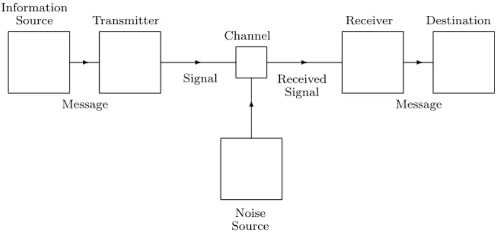
Figure 1.1: Shannon’s model of communication Information Source -Message Transmitter -Signal Channel -Received Signal Receiver -Message Destination 6 Noise Source

1.2

General communication systems

We begin with Shannon’s model of a general communication system, Figure 1.2. This setup is sufficiently general to handle many communication situations. Most other communication models, such as those requiring feedback, will start with this model as their base.

Our primary concern is block coding for error correction on a discrete mem-oryless channel. We next describe these and other basic assumptions that are made here concerning various of the parts of Shannon’s system; see Figure 1.2. As we note along the way, these assumptions are not the only ones that are valid or interesting; but in studying them we will run across most of the com-mon issues of coding theory. We shall also honor these assumptions by breaking them periodically.

We shall usually speak of the transmission and reception of the words of the code, although these terms may not be appropriate for a specific envisioned ap-plication. For instance, if we are mainly interested in errors that affect computer memory, then we might better speak of storage and retrieval.

1.2.1

Message

Our basic assumption on messages is that each possible message k-tuple is as likely to be selected for broadcast as any other.

We are thus ignoring the concerns of source coding. Perhaps a better way to say this is that we assume source coding has already been done for us. The original message has been source coded into a set of k-tuples, each equally likely. This is not an unreasonable assumption, since lossless source coding is designed to do essentially this. Beginning with an alphabet in which different

(14)

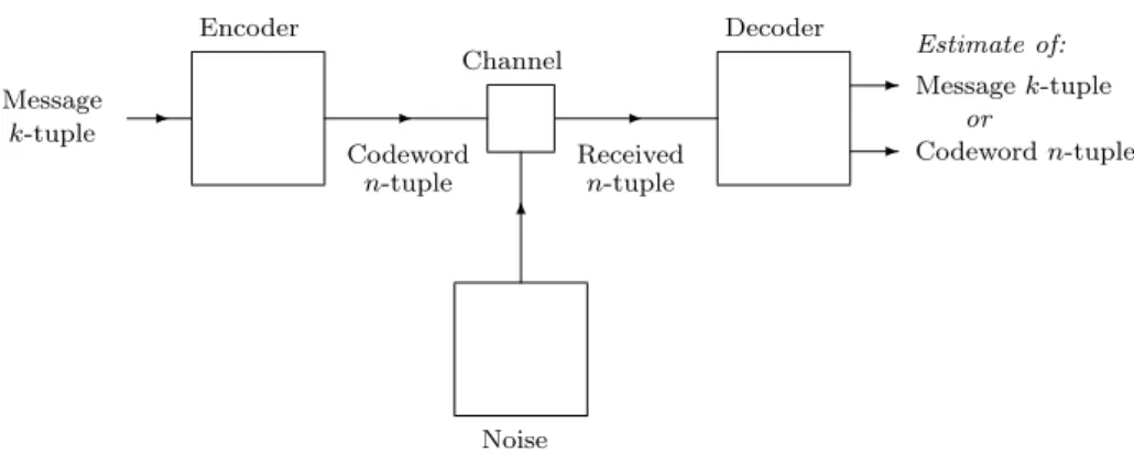
Figure 1.2: A more specific model -Message k-tuple Encoder -Codeword n-tuple Channel -Received n-tuple Decoder -Estimate of: Messagek-tuple or Codewordn-tuple 6 Noise

letters have different probabilities of occurrence, source coding produces more compact output in which frequencies have been levelled out. In a typical string of Morse code, there will be roughly the same number of dots and dashes. If the letter “e” was mapped to two dots instead of one, we would expect most strings to have a majority of dots. Those strings rich in dashes would be effectively ruled out, so there would be fewer legitimate strings of any particular reasonable length. A typical message would likely require a longer encoded string under this new Morse code than it would with the original. Shannon made these observations precise in his Source Coding Theorem which states that, beginning with an ergodic message source (such as the written English language), after proper source coding there is a set of source encoded k-tuples (for a suitably largek) which comprises essentially allk-tuples and such that different encoded k-tuples occur with essentially equal likelihood.

1.2.2

Encoder

We are concerned here withblock coding. That is, we transmit blocks of symbols block coding

of fixed lengthnfrom a fixed alphabetA. These blocks are the codewords, and that codeword transmitted at any given moment depends only upon the present message, not upon any previous messages or codewords. Our encoder has no memory. We also assume that each codeword from the code (the set of all possible codewords) is as likely to be transmitted as any other.

Some work has been done on codes over mixed alphabets, that is, allowing the symbols at different coordinate positions to come from different alphabets. Such codes occur only in isolated situations, and we shall not be concerned with them at all.

(15)

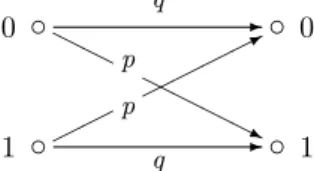
en-Figure 1.3: The Binary Symmetric Channel c c c c 1 0 1 0 * H H H H H H j q q p p

coders that have memory. We lump these together under the heading of

con-volutional codes. The message string arrives at the decoder continuously rather convolutional codes than segmented into unrelated blocks of lengthk, and the code string emerges

continuously as well. That n-tuple of code sequence that emerges from the en-coder while a given k-tuple of message is being introduced will depend upon previous message symbols as well as the present ones. The encoder “remem-bers” earlier parts of the message. The coding most often used in modems is of convolutional type.

1.2.3

Channel

As already mentioned, we shall concentrate on coding on adiscrete memoryless

channelor DMC. The channel is discrete because we shall only consider finite discrete memoryless channel

DMC

alphabets. It is memoryless in that an error in one symbol does not affect the reliability of its neighboring symbols. The channel has no memory, just as above we assumed that the encoder has no memory. We can thus think of the channel as passing on the codeword symbol-by-symbol, and the characteristics of the channel can described at the level of the symbols.

An important example is furnished by the m-ary symmetric channel. The

m-ary symmetric channelhas input and output an alphabet ofmsymbols, say m-ary symmetric channel x1, . . . , xm. The channel is characterized by a single parameterp, the

probabil-ity that after transmission of any symbol xj the particular symbol xi 6=xj is

received. That is,

p= Prob(xi|xj), fori6=j .

Related are the probability

s= (m−1)p

that afterxj is transmitted it is not received correctly and the probability

q= 1−s= 1−(m−1)p= Prob(xj|xj))

that afterxj is transmitted it is received correctly. We writemSC(p) for them- mSC(p)

ary symmetric channel withtransition probability p. The channel is symmetric transition probability in the sense Prob(xi|xj) does not depend upon the actual values ofiandjbut

only on whether or not they are equal. We are especially interested in the 2-ary

symmetric channel or binary symmetric channel BSC(p) (wherep=s). BSC(p)

Of course the signal that is actually broadcast will often be a measure of some frequency, phase, or amplitude, and so will be represented by a real (or complex)

(16)

number. But usually only a finite set of signals is chosen for broadcasting, and the members of a finite symbol alphabet are modulated to the members of the finite signal set. Under our assumptions the modulator is thought of as part of the channel, and the encoder passes symbols of the alphabet directly to the channel.

There are other situations in which a continuous alphabet is the most ap-propriate. The most typical model is aGaussian channelwhich has as alphabet Gaussian channel

an interval of real numbers (bounded due to power constraints) with errors introduced according to a Gaussian distribution.

The are also many situations in which the channel errors exhibit some kind of memory. The most common example of this is burst errors. If a particular symbol is in error, then the chances are good that its immediate neighbors are also wrong. In telephone transmission such errors occur because of lightening and crosstalk. A scratch on a compact disc produces burst errors since large blocks of bits are destroyed. Of course a burst error can be viewed as just one type of random error pattern and be handled by the techniques that we shall develop. We shall also see some methods that are particularly well suited to dealing with burst errors.

One final assumption regarding our channel is really more of a rule of thumb. We should assume that the channel machinery that carries out modulation, transmission, reception, and demodulation is capable of reproducing the trans-mitted signal with decent accuracy. We have a

Reasonable Assumption— Most errors that occur are not severe. Otherwise the problem is more one of design than of coding. For aDM C we interpret the reasonable assumption as saying that an error pattern composed of a small number of symbol errors is more likely than one with a large number. For a continuous situation such as the Gaussian channel, this is not a good viewpoint since it is nearly impossible to reproduce a real number with perfect accuracy. All symbols are likely to be received incorrectly. Instead we can think of the assumption as saying that whatever is received should resemble to a large degree whatever was transmitted.

1.2.4

Received word

We assume that the decoder receives from the channel an n-tuple of symbols from the transmitter’s alphabetA.

This assumption could be included in our discussion of the channel, since it really concerns the demodulator, which we think of as part of the chan-nel just as we do the modulator. Many implementations combine the de-modulator with the decoder in a single machine. This is the case with com-puter modems which serve as encoder/modulator and demodulator/decoder (MOdulator-DEModulator).

Think about how the demodulator works. Suppose we are using a binary alphabet which the modulator transmits as signals of amplitude +1 and −1. The demodulator receives signals whose amplitudes are then measured. These

(17)

received amplitudes will likely not be exactly +1 or −1. Instead values like .750, and−.434 and.003 might be found. Under our assumptions each of these must be translated into a +1 or −1 before being passed on to the decoder. An obvious way of doing this is to take positive values to +1 and negative values to −1, so our example string becomes +1,−1,+1. But in doing so, we have clearly thrown away some information which might be of use to the decoder. Suppose in decoding it becomes clear that one of the three received symbols is certainly not the one originally transmitted. Our decoder has no way of deciding which one to mistrust. But if the demodulator’s knowledge were available, the decoder would know that the last symbol is the least reliable of the three while the first is the most reliable. This improves our chances of correct decoding in the end. In fact with our assumption we are asking the demodulator to do some initial, primitive decoding of its own. The requirement that the demodulator

make precise (or hard) decisions about code symbols is calledhard quantization. hard quantization The alternative issoft quantization. Here the demodulator passes on information soft quantization which suggests which alphabet symbol might have been received, but it need not

make a final decision. At its softest, our demodulator would pass on the three real amplitudes and leave all symbol decisions to the decoder. This of course involves the least loss of information but may be hard to handle. A mild but

still helpful form of soft quantization is to allow channelerasures. The channel erasures receives symbols from the alphabetAbut the demodulator is allowed to pass on

to the decoder symbols fromA∪ {?}, where the special symbol “?” indicates an inability to make an educated guess. In our three symbol example above, the decoder might be presented with the string +1,−1,?, indicating that the last symbol was received unreliably. It is sometimes helpful to think of an erasure as a symbol error whose location is known.

1.2.5

Decoder

Suppose that in designing our decoding algorithms we know, for each n-tuple y and each codeword x, the probability p(y|x) that y is received after the transmission ofx. The basis of our decoding is the following principle:

Maximum Likelihood Decoding— Whenyis received, we must decode to a codewordxthat maximizes Prob(y|x).

We often abbreviate this toMLD. While it is very sensible, it can cause prob- MLD

lems similar to those encountered during demodulation. Maximum likelihood decoding is “hard” decoding in that we must always decode to some codeword.

This requirement is calledcomplete decoding. complete decoding

The alternative to complete decoding is incomplete decoding, in which we incomplete decoding either decode a received n-tuple to a codeword or to a new symbol ∞ which

could be read as “errors were detected but were not corrected” (sometimes

ab-breviated to “error detected”). Sucherror detection(as opposed to correction) error detection can come about as a consequence of adecoding default. We choose this default decoding default alternative when we are otherwise unable (or unwilling) to make a sufficiently

(18)

of length 26 (rather than 27 as before), then majority vote still deals effectively with 12 or fewer errors; but 13 errors produces a 13 to 13 tie. Rather than make an arbitrary choice, it might be better to announce that the received message is too unreliable for us to make a guess. There are many possible actions upon default. Retransmission could be requested. There may be other “nearby” data that allows an undetected error to be estimated in other ways. For instance, with compact discs the value of the uncorrected sound level can be guessed to be the average of nearby values. (A similar approach can be take for digital images.) We will often just declare “error detected but not corrected.”

Almost all the decoding algorithms that we discuss in detail will not be MLDbut will satisfyIMLD, the weaker principle:

IMLD

Incomplete Maximum Likelihood Decoding — When y is received, we must decode either to a codeword x that maximizes Prob(y|x) or to the “error detected” symbol∞.

Of course, if we are only interested in maximizing our chance of successful decoding, then any guess is better than none; and we should useMLD. But this longshot guess may be hard to make, and if we are wrong then the consequences might be worse than accepting but recognizing failure. When correct decoding is not possible or advisable, this sort of error detection is much preferred over making an error in decoding. Adecoder errorhas occurred ifxhas been trans-decoder error

mitted,y received and decoded to a codewordz6=x. A decoder error is much less desirable than a decoding default, since to the receiver it has the appear-ance of being correct. With detection we know something has gone wrong and can conceivably compensate, for instance, by requesting retransmission. Finally decoder failureoccurs whenever we do not have correct decoding. Thus decoder decoder failure

failure is the combination of decoding default and decoder error.

Consider a codeCinAnand a decoding algorithmA. ThenPx(A) is defined as the error probability (more properly, failure probability) that afterx∈C is transmitted, it is received and not decoded correctly usingA. We then define

PC(A) =|C|−1 X

x∈C

Px(A),

the average error expectation for decodingCusing the algorithmA. This judges how good A is as an algorithm for decoding C. (Another good gauge would be the worst case expectation, maxx∈CPx(A).) We finally define the error

expectationPC forCvia

error expectationPC

PC = min

A PC(A).

IfPC(A) is large then the algorithm is not good. IfPCis large, then no decoding

algorithm is good for C; and soC itself is not a good code. In fact, it is not hard to see thatPC=PC(A), for everyMLDalgorithmA. (It would be more

consistent to call PC the failure expectation, but we stick with the common

terminology.)

We have already remarked upon the similarity of the processes of demodu-lation and decoding. Under this correspondence we can think of the detection

(19)

symbol∞as the counterpart to the erasure symbol?while decoder errors cor-respond to symbol errors. Indeed there are situations in concatenated coding where this correspondence is observed precisely. Codewords emerging from the “inner code” are viewed as symbols by the “outer code” with decoding error and default becoming symbol error and erasure as described.

A main reason for using incomplete rather than complete decoding is ef-ficiency of implementation. An incomplete algorithm may be much easier to implement but only involve a small degradation in error performance from that for complete decoding. Again consider the length 26 repetition code. Not only are patterns of 13 errors extremely unlikely, but they require different handling than other types of errors. It is easier just to announce that an error has been detected at that point, and the the algorithmic error expectation PC(A) only

increases by a small amount.

1.3

Some examples of codes

1.3.1

Repetition codes

These codes exist for any lengthnand any alphabetA. A message consists of a letter of the alphabet, and it is encoded by being repeatedntimes. Decoding can be done by plurality vote, although it may be necessary to break ties arbitrarily. The most fundamental case is that of binary repetition codes, those with alphabet A = {0,1}. Majority vote decoding always produces a winner for binary repetition codes of odd length. The binary repetition codes of length 26 and 27 were discussed above.

1.3.2

Parity check and sum-

0

codes

Parity check codes form the oldest family of codes that have been used in prac-tice. The parity check code of length n is composed of all binary (alphabet A ={0,1})n-tuples that contain an even number of 1’s. Any subset ofn−1 coordinate positions can be viewed as carrying the information, while the re-maining position “checks the parity” of the information set. The occurrence of a single bit error can be detected since the parity of the received n-tuple will be odd rather than even. It is not possible to decide where the error occurred, but at least its presence is felt. (The parity check code is able to correct single erasures.)

The parity check code of length 27 was discussed above.

A versions of the parity check code can be defined in any situation where the alphabet admits addition. The code is then all n-tuples whose coordinate entries sum to 0. When the alphabet is the integers modulo 2, we get the usual parity check code.

1.3.3

The

[7,

4]

binary Hamming code

(20)

An efficient code, allowing complete correction of [single] errors and transmitting at the rateC [= 4/7], is the following (found by a method due to R. Hamming):

Let a block of seven symbols be X1, X2, . . . , X7 [each either 0 or 1]. Of theseX3, X5, X6, andX7 are message symbols and cho-sen arbitrarily by the source. The other three are redundant and calculated as follows:

X4is chosen to makeα = X4+X5+X6+X7 even X2is chosen to make β = X2+X3+X6+X7 even X1is chosen to make γ = X1+X3+X5+X7 even When a block of seven is received, α,β, andγare calculated and if even called zero, if odd called one. The binary number α β γ then gives the subscript of the Xi that is incorrect (if 0 then there was

no error).

This describes a [7,4] binary Hamming code together with its decoding. We shall give the general versions of this code and decoding in a later chapter.

R.J. McEliece has pointed out that the [7,4] Hamming code can be nicely thought of in terms of the usual Venn diagram:

&% '$ &% '$ &% '$ X1 X7 X6 X4 X2 X5 X3

The message symbols occupy the center of the diagram, and each circle is com-pleted to guarantee that it contains an even number of 1’s (has even parity). If, say, received circlesAandB have odd parity but circleChas even parity, then the symbol withinA∩B∩C is judged to be in error at decoding.

1.3.4

An extended binary Hamming code

An extension of a binary Hamming code results from adding at the beginning of each codeword a new symbol that checks the parity of the codeword. To the [7,4] Hamming code we add an initial symbol:

X0is chosen to makeX0+X1+X2+X3+X4+X5+X6+X7 even The resulting code is the [8,4] extended Hamming code. In the Venn diagram the symbolX0 checks the parity of the universe.

The extended Hamming code not only allows the correction of single errors (as before) but also detects double errors.

(21)

&% '$ &% '$ &% '$ X0 X1 X7 X6 X4 X2 X5 X3

1.3.5

The

[4,

2]

ternary Hamming code

This is a code of nine 4-tuples (a, b, c, d) ∈ A4 _{with ternary alphabet} _A ₌ {0,1,2}. Endow the setA with the additive structure of the integers modulo 3. The first two coordinate positionsa, bcarry the 2-tuples of information, each pair (a, b)∈ A2 _{exactly once (hence nine codewords). The entry in the third} position is sum of the previous two (calculated, as we said, modulo 3):

a+b=c ,

for instance, with (a, b) = (1,0) we get c= 1 + 0 = 1. The final entry is then selected to satisfy

b+c+d= 0,

so that 0 + 1 + 2 = 0 completes the codeword (a, b, c, d) = (1,0,1,2). These two equations can be interpreted as making ternary parity statements about the codewords; and, as with the binary Hamming code, they can then be exploited for decoding purposes. The complete list of codewords is:

(0,0,0,0) (1,0,1,2) (2,0,2,1) (0,1,1,1) (1,1,2,0) (2,1,0,2) (0,2,2,2) (1,2,0,1) (2,2,1,0)

( 1.3.1 ) Problem. Use the two defining equations for this ternary Hamming code to describe a decoding algorithm that will correct all single errors.

1.3.6

A generalized Reed-Solomon code

We now describe a code of lengthn= 27 with alphabet the field of real number R. Given our general assumptions this is actually a nonexample, since the alphabet is not discrete or even bounded. (There are, in fact, situations where these generalized Reed-Solomon codes with real coordinates have been used.)

Choose 27 distinct real numbersα1, α2, . . . , α27. Our messagek-tuples will be 7-tuples of real numbers (f0, f1, . . . , f6), so k = 7. We will encode a given message 7-tuple to the codeword 27-tuple

(22)

where

f(x) =f0+f1x+f2x2+f3x3+f4x4+f5x5+f6x6

is the polynomial function whose coefficients are given by the message. Our Reasonable Assumption says that a received 27-tuple will resemble the codeword transmitted to a large extent. If a received word closely resembles each of two codewords, then they also resemble each other. Therefore to achieve a high probability of correct decoding we would wish pairs of codewords to be highly dissimilar.

The codewords coming from two different messages will be different in those coordinate positionsi at which their polynomialsf(x) andg(x) have different values at αi. They will be equal at coordinate position i if and only ifαi is a

root of the difference h(x) =f(x)−g(x). But this can happen for at most 6 values ofisinceh(x) is a nonzero polynomial of degree at most 6. Therefore:

distinct codewords differ in at least 21 (= 27−6) coordinate posi-tions.

Thus two distinct codewords are highly different. Indeed as many up to 10 errors can be introduced to the codewordf forf(x) and the resulting word will still resemble the transmitted codewordf more than it will any other codeword. The problem with this example is that, given our inability in practice to describe a real number with arbitrary accuracy, when broadcasting with this code we must expect almost all symbols to be received with some small error — 27 errors every time! One of our later objectives will be to translate the spirit of this example into a more practical setting.

(23)

Chapter 2

Sphere Packing and

Shannon’s Theorem

In the first section we discuss the basics of block coding on them-ary symmetric channel. In the second section we see how the geometry of the codespace can be used to make coding judgements. This leads to the third section where we present some information theory and Shannon’s basic Channel Coding Theorem.

2.1

Basics of block coding on the

m

SC

Let Abe any finite set. A block codeor code, for short, will be any nonempty block code subset of the set An _of _{n-tuples of elements from}_{A. The number} _n₌_{n(C) is}

thelengthof the code, and the setAn _{is the}_codespace_{. The number of members} _length

codespace in C is thesizeand is denoted|C|. IfChas length nand size|C|, we say that

size C is an (n,|C|)code.

(n,|C|)code The members of the codespace will be referred to aswords, those belonging

words to Cbeing codewords. The setAis then thealphabet.

codewords alphabet If the alphabetA hasm elements, then C is said to be anm-ary code. In

m-ary code the special case |A|=2 we say C is a binary code and usually take A={0,1}

binary or A = {−1,+1}. When |A|=3 we say C is aternary code and usually take

ternary A ={0,1,2} orA ={−1,0,+1}. Examples of both binary and ternary codes

appeared in Section 1.3.

For a discrete memoryless channel, the Reasonable Assumption says that a pattern of errors that involves a small number of symbol errors should be more likely than any particular pattern that involves a large number of symbol errors. As mentioned, the assumption is really a statement about design.

On anmSC(p) the probabilityp(y|x) thatxis transmitted andyis received is equal to pd_qn−d_{, where} _d _{is the number of places in which} _x _and _y _differ.

Therefore

Prob(y|x) =qn(p/q)d, 15

(24)

a decreasing function ofdprovidedq > p. Therefore the Reasonable Assumption is realized by themSC(p) subject to

q= 1−(m−1)p > p or, equivalently,

1/m > p .

We interpret this restriction as the sensible design criterion that after a symbol is transmitted it should be more likely for it to be received as the correct symbol than to be received as any particular incorrect symbol.

Examples.

(i) Assume we are transmitting using the the binary Hamming code of Section 1.3.3 on BSC(.01). Comparing the received word 0011111 with the two codewords 0001111 and 1011010 we see that

p(0011111|0001111) =q6p1≈.009414801,

while

p(0011111|1011010) =q4p3≈.000000961 ;

therefore we prefer to decode 0011111 to 0001111. Even this event is highly unlikely, compared to

p(0001111|0001111) =q7≈.932065348.

(ii) If m = 5 withA ={0,1,2,3,4}6 _and_p ₌_.₀₅_<₁_/_{5 =} _._{2, then} q= 1−4(.05) =.8; and we have

p(011234|011234) =q6=.262144 and

p(011222|011234) =q4p2=.001024. Forx,y∈An, we define

dH(x,y) = the number of places in whichxandydiffer.

This number is theHamming distancebetweenxandy. The Hamming distance Hamming distance

is a genuine metric on the codespaceAn_{. It is clear that it is symmetric and}

that dH(x,y) = 0 if and only ifx=y. The Hamming distance dH(x,y) should be thought of as the number of errors required to changexinto y(or, equally well, to changeyinto x).

Example.

dH(0011111,0001111) = 1 ;

dH(0011111,1011010) = 3 ;

dH(011234,011222) = 2.

( 2.1.1 )_Problem. Prove the triangle inequality for the Hamming distance:

(25)

The arguments above show that, for anmSC(p) withp <1/m, maximum likelihood decoding becomes:

Minimum Distance Decoding— When y is received, we must decode to a codewordxthat minimizes the Hamming distance dH(x,y).

We abbreviate minimum distance decoding as MDD. In this context, incom- minimum distance decoding

MDD

plete decoding is incomplete minimum distance decodingIMDD:

IMDD

Incomplete Minimum Distance Decoding — When y is re-ceived, we must decode either to a codeword xthat minimizes the Hamming distance dH(x,y) or to the “error detected” symbol∞.

( 2.1.2 )Problem. Prove that, for anmSC(p)withp= 1/m, every complete decoding algorithm is anMLDalgorithm.

( 2.1.3 ) _Problem. Give a definition of what might be called maximum distance decoding, MxDD; and prove that MxDD algorithms are MLD algorithms for an mSC(p) withp >1/m.

InAn, thesphere1 of radiusρcentered atxis sphere Sρ(x) ={y∈An|dH(x,y)≤ρ}.

Thus the sphere of radius ρ around x is composed of those y that might be received if at mostρsymbol errors were introduced to the transmitted codeword x.

The volume of a sphere of radius ρ is independent of the location of its center.

( 2.1.4 ) _Problem. Prove that in An _with _|_A_|₌_m_{, a sphere of radius} _e _contains e X i=0 n i ! (m−1)i words.

For example, a sphere of radius 2 in{0,1}90_{has volume} 1 + ₉₀ 1 + ₉₀ 2 = 1 + 90 + 4005 = 4096 = 212

corresponding to a center, 90 possible locations for a single error, and 90₂

possibilities for a double error. A sphere of radius 2 in{0,1,2}8 _{has volume} 1 + ₈ 1 (3−1)1+ ₈ 2 (3−1)2= 1 + 16 + 112 = 129.

For each nonnegative real numberρwe define a decoding algorithmSSρ for SSρ

An _called_{sphere shrinking}_.

sphere shrinking 1_{Mathematicians would prefer to use the term ‘ball’ here in place of ‘sphere’, but we stick}

(26)

Radius ρ Sphere Shrinking — If y is received, we decode to the codewordx ifxis the unique codeword in Sρ(y), otherwise we

declare a decoding default.

Thus SSρ shrinks the sphere of radius ρ around each codeword to its center,

throwing out words that lie in more than one such sphere.

The various distance determined algorithms are completely described in terms of the geometry of the codespace and the code rather than by the specific channel characteristics. In particular they no longer depend upon the transi-tion parameterpof an mSC(p) being used. ForIMDD algorithmsA andB, if PC(A) ≤ PC(B) for some mSC(p) with p < 1/m, then PC(A) ≤ PC(B)

will be true for allmSC(p) withp <1/m. TheIMDD algorithms are (incom-plete) maximum likelihood algorithms on everymSC(p) withp≤1/m, but this observation now becomes largely motivational.

Example. Consider the specific case of a binary repetition code of

length 26. Since the first two possibilities are not algorithms but classes of algorithms there are choices available.

w= number of 1’s 0 1≤w≤11 = 12 = 13 = 14 15≤w≤25 26 IMDD 0/∞ 0/∞ 0/∞ 0/1/∞ 1/∞ 1/∞ 1/∞ MDD 0 0 0 0/1 1 1 1 SS12 0 0 0 ∞ 1 1 1 SS11 0 0 ∞ ∞ ∞ 1 1 SS0 0 ∞ ∞ ∞ ∞ ∞ 1

Here0and1denote, respectively, the 26-tuple of all 0’s and all 1’s. In the fourth case, we have less error correcting power. On the other hand we are less likely to have a decoder error, since 15 or more symbol errors must occur before a decoder error results. The final case corrects no errors, but detects nontrivial errors except in the extreme case where all symbols are received incorrectly, thereby turning the transmitted codeword into the other codeword.

The algorithm SS0 used in the example is the usual error detection algo-rithm: whenyis received, decode toyif it is a codeword and otherwise decode to∞, declaring that an error has been detected.

2.2

Sphere packing

The code C in An _has _{minimum distance} _{dmin(C) equal to the minimum of}

minimum distance

dH(x,y), asx and y vary over all distinct pairs of codewords from C. (This leaves some confusion over dmin(C) for a lengthncodeCwith only one word. It may be convenient to think of it as any number larger thann.) An (n, M) code with minimum distancedwill sometimes be referred to as an (n, M, d)code.

(n, M, d)code

Example. The minimum distance of the repetition code of lengthnis clearlyn. For the parity check code any single error produces a word of

(27)

odd parity, so the minimum distance is 2. The length 27 generalized Reed-Solomon code of Example 1.3.6 was shown to have minimum distance 21. Laborious checking reveals that the [7,4] Hamming code has minimum distance 3, and its extension has minimum distance 4. The [4,2] ternary Hamming code also has minimum distance 3. We shall see later how to find the minimum distance of these codes easily.

( 2.2.1 ) _Lemma. The following are equivalent for the code C in An _{for an}

integer e≤n:

(1) under SSe any occurrence of e or fewer symbol errors will always be

successfully corrected;

(2)for all distinct x,yin C, we have Se(x)∩Se(y) =∅;

(3)the minimum distance of C,dmin(C), is at least2e+ 1.

Proof.Assume (1), and letz∈Se(x), for somex∈C. Then by assumption

zis decoded toxbySSe. Therefore there is noy∈Cwithy6=xandz∈Se(y),

giving (2).

Assume (2), and let z be a word that results from the introduction of at mosteerrors to the codewordx. By assumptionzis not in Se(y) for anyy of

C other than x. Therefore, Se(z) contains x and no other codewords; soz is

decoded toxbySSe, giving (1).

If z ∈ Se(x)∩Se(y), then by the triangle inequality we have dH(x,y) ≤

dH(x,z) + dH(z,y)≤2e, so (3) implies (2).

It remains to prove that (2) implies (3). Assume dmin(C) =d≤2e. Choose x= (x1, . . . , xn) and y= (y1, . . . , yn) inC with dH(x,y) =d. Ifd≤e, then x∈Se(x)∩Se(y); so we may suppose that d > e.

Leti1, . . . , id≤nbe the coordinate positions in whichxandydiffer: xij 6= yij, for j= 1, . . . , d. Definez= (z1, . . . , zn) by zk =yk ifk6∈ {i1, . . . , ie} and zk =xk ifk∈ {i1, . . . , ie}. Then dH(y,z) =eand dH(x,z) =d−e≤e. Thus z∈Se(x)∩Se(y). Therefore (2) implies (3). 2

A code C that satisfies the three equivalent properties of Lemma 2.2.1 is

called an e-error-correcting code. The lemma reveals one of the most pleasing e-error-correcting code aspects of coding theory by identifying concepts from three distinct and

impor-tant areas. The first property is algorithmic, the second is geometric, and the third is linear algebraic. We can readily switch from one point of view to another in search of appropriate insight and methodology as the context requires.

( 2.2.2 ) Problem. Explain why the error detecting algorithm SS0 correctly detects all patterns of fewer than dmin symbol errors.

( 2.2.3 )Problem. Letf≥e. Prove that the following are equivalent for the codeC inAn_:

(1)underSSeany occurrence ofeor fewer symbol errors will always be successfully

corrected and no occurrence of f or fewer symbol errors will cause a decoder error;

(2)for all distinct x,y inC, we have Sf(x)∩Se(y) =∅;

(3)the minimum distance ofC,dmin(C), is at leaste+f+ 1.

A code C that satisfies the three equivalent properties of the problem is called an e

-error-correcting,f-error-detectingcode. e-error-correcting, f-error-detecting

(28)

( 2.2.4 ) _Problem. Consider an erasure channel, that is, a channel that erases certain symbols and leaves a ‘?’ in their place but otherwise changes nothing. Explain why, using a code with minimum distancedon this channel, we can correct all patterns of up tod−1symbol erasures. (In certain computer systems this observation is used to protect against hard disk crashes.)

By Lemma 2.2.1, if we want to construct an e-error-correcting code, we must be careful to choose as codewords the centers of radiusespheres that are pairwise disjoint. We can think of this as packing spheres of radiuse into the large box that is the entire codespace. From this point of view, it is clear that we will not be able to fit in any number of spheres whose total volume exceeds the volume of the box. This proves:

( 2.2.5 )_{Theorem. (Sphere packing condition.)} IfCis ane-error-correcting code inAn_{, then}

|C| · |Se(∗)| ≤ |An|. 2

Combined with Problem 2.1.4, this gives:

( 2.2.6 ) _{Corollary. (Sphere packing bound; Hamming bound.)} If C is am-arye-error-correcting code of lengthn, then

|C| ≤mn e X i=0 _n i (m−1)i. 2

A code C that meets the sphere packing bound with equality is called a perfect e-error-correcting code. Equivalently, C is a perfect e-error-correcting perfecte-error-correcting code

code if and only ifSSe is aMDDalgorithm. As examples we have the binary

repetition codes of odd length. The [7,4] Hamming code is a perfect 1-error-correcting code, as we shall see in Section 4.1.

( 2.2.7 ) Theorem. (Gilbert-Varshamov bound.) There exists an m-ary e-error-correcting codeC of lengthn such that

|C| ≥mn 2e X i=0 _n i (m−1)i.

Proof. The proof is by a “greedy algorithm” construction. Let the

code-space be An_{. At} _Step _{1 we begin with the code}_C1 ₌_{x

1}, for any word x1. Then, fori≥2, we have:

Stepi.SetSi=S i−1

j=1Sd−1(xj).

IfSi =An, halt.

Otherwise choose a vector xi inAn−Si;

set Ci=Ci−1∪ {xi};

(29)

AtStepi, the codeCihas cardinalityiand is designed to have minimum distance

at leastd. (As long asd≤nwe can choose x2 at distancedfrom x1; so each Ci, fori≥1 has minimum distance exactlyd.)

How soon does the algorithm halt? We argue as we did in proving the sphere packing condition. The set Si =S_ji−₌₁1Sd−1(xj) will certainly be smaller than

An _{if the spheres around the words of} _C

i−1 have total volume less than the volume of the entire spaceAn_{; that is, if}

|Ci−1| · |Sd−1(∗)|<|An|.

Therefore when the algorithm halts, this inequality must be false. Now Problem

2.1.4 gives the bound. 2

A sharper version of the Gilbert-Varshamov bound exists, but the asymptotic result of the next section is unaffected.

Examples.

(i) Consider a binary 2-error-correcting code of length 90. By the Sphere Packing Bound it has size at most

290 |S2(∗)| = 2 90 212 = 2 78 .

If a code existed meeting this bound, it would be perfect. By the Gilbert-Varshamov Bound, in {0,1}90

there exists a code C

with minimum distance 5, which therefore corrects 2 errors, and having

|C| ≥ 2 90 |S4(∗)| = 2 90 2676766 ≈4.62×10 20 .

As 278≈3.02×1023, there is a factor of roughly 650 separating the lower and upper bounds.

(ii) Consider a ternary 2-error-correcting code of length 8. By the Sphere Packing Bound it has size bounded above by

38

|S2(∗)|

= 6561

129 ≈50.86.

Therefore it has size at mostb50.86c= 50. On the other hand, the Gilbert-Varshamov Bound guarantees only a codeC of size bounded below by

|C| ≥ 6561 |S4(∗)|

= 6561

1697≈3.87,

that is, of size at leastd3.87e= 4 ! Later we shall construct an appropriate

Cof size 27. (This is in fact the largest possible.)

( 2.2.8 )_Problem. In each of the following cases decide whether or not there exists a

1-error-correcting codeCwith the given size in the codespaceV. If there is such a code, give an example (except in(d), where an example is not required but a justification is). If there is not such a code, prove it.

(a) V ={0,1}5 and|C|= 6; (b)V ={0,1}6 and|C|= 9; (c)V ={0,1,2}4 and|C|= 9. (d) V ={0,1,2}8 _and_|_C_|_{= 51}_.

(30)

( 2.2.9 )_Problem. In each of the following cases decide whether or not there exists a2-error-correcting code C with the given size in the codespaceV. If there is such a code, give an example. If there is not such a code, prove it.

(a)V ={0,1}8

and|C|= 4;

(b)V ={0,1}8 _and_|_C_|_{= 5}_.

2.3

Shannon’s theorem and the code region

The present section is devoted to information theory rather than coding theory and will not contain complete proofs. The goal of coding theory is to live up to the promises of information theory. Here we shall see of what our dreams are made.

Our immediate goal is to quantify the Fundamental Problem. We need to evaluate information content and error performance.

We first consider information content. The m-ary code C has dimension dimension

k(C) = log_m(|C|). The integer k = dk(C)e is the smallest such that each message for Ccan be assigned its own individual message k-tuple from the m-ary alphabet A. Therefore we can think of the dimension as the number of codeword symbols that are carrying message rather than redundancy. (Thus the numbern−kis sometimes called theredundancyof C.) A repetition code redundancy

hasnsymbols, only one of which carries the message; so its dimension is 1. For a length n parity check code, n−1 of the symbols are message symbols; and so the code has dimension n−1. The [7,4] Hamming code has dimension 4 as does its [8,4] extension, since both contain 24 _{= 16 codewords. Our definition} of dimension does not apply to our real Reed-Solomon example 1.3.6 since its alphabet is infinite, but it is clear what its dimension should be. Its 27 positions are determined by 7 free parameters, so the code should have dimension 7.

The dimension of a code is a deceptive gauge of information content. For instance, a binary codeCof length 4 with 4 codewords and dimension log₂(4) = 2 actually contains more information than a second codeD of length 8 with 8 codewords and dimension log₂(8) = 3. Indeed the codeCcan be used to produce 16 = 4×4 different valid code sequences of length 8 (a pair of codewords) while the code D only offers 8 valid sequences of length 8. Here and elsewhere, the proper measure of information content should be the fraction of the code symbols that carries information rather than redundancy. In this example 2/4 = 1/2 of the symbols ofC carry information while for D only 3/8 of the symbols carry information, a fraction smaller than that forC.

The fraction of a repetition codeword that is information is 1/n, and for a parity check code the fraction is (n−1)/n. In general, we define thenormalized dimensionor rateκ(C) of them-ary codeC of lengthnby

rate

κ(C) =k(C)/n=n−1log_m(|C|).

The repetition code thus has rate 1/n, and the parity check code rate (n−1)/n. The [7,4] Hamming code has rate 4/7, and its extension rate 4/8 = 1/2. The [4,2] ternary Hamming code has rate 2/4 = 1/2. Our definition of rate does

(31)

not apply to the real Reed-Solomon example of 1.3.6, but arguing as before we see that it has “rate” 7/27. The rate is the normalized dimension of the code, in that it indicates the fraction of each code coordinate that is information as opposed to redundancy.

The rateκ(C) provides us with a good measure of the information content of C. Next we wish to measure the error handling ability of the code. One possible gauge is PC, the error expectation of C; but in general this will be

hard to calculate. We can estimatePC, for anmSC(p) with smallp, by making

use of the obvious relationship PC ≤ PC(SSρ) for any ρ. If e =b(d−1)/2c,

thenCis ane-error-correcting code; and certainlyPC≤ PC(SSe), a probability

that is easy to calculate. IndeedSSe corrects all possible patterns of at moste

symbol errors but does not correct any other errors; so PC(SSe) = 1− e X i=0 _n i (m−1)ipiqn−i.

The difference betweenPC andPC(SSe) will be given by further termspjqn−j

withj larger than e. For smallp, these new terms will be relatively small. Shannon’s theorem guarantees the existence of large families of codes for whichPCis small. The previous paragraph suggests that to prove this efficiently

we might look for codes with arbitrarily smallPC(SS(dmin−1)/2), and in a sense

we do. However, it can be proven that decoding up to minimum distance alone is not good enough to prove Shannon’s Theorem. (Think of the ‘Birthday Paradox’.) Instead we note that a received block of large lengthnis most likely to contain sn symbol errors where s = p(m−1) is the probability of symbol error. Therefore in proving Shannon’s theorem we look at large numbers of codes, each of which we decode usingSSρ for some radiusρa little larger than

sn.

A familyC of codes over A is called a Shannon family if, for every > 0, Shannon family there is a codeC∈ C with PC< . For a finite alphabetA, the familyC must

necessarily be infinite and so contain codes of unbounded length.

( 2.3.1 ) Problem. Prove that the set of all binary repetition codes of odd length is a Shannon family onBSC(p)forp <1/2.

Although repetition codes give us a Shannon family, they do not respond to the Fundamental Problem by having good information content as well. Shannon proved that codes of the sort we need are out there somewhere.

( 2.3.2 )_{Theorem. (Shannon’s Channel Coding Theorem.)} Consider the m-ary symmetric channel mSC(p) with p < 1/m. There is a function Cm(p)

such that, for any κ < Cm(p),

Cκ ={ m-ary block codes of rate at least κ}

is a Shannon family. Conversely ifκ > Cm(p), thenCκis not a Shannon family.

(32)

The functionCm(p) is the capacity function for themSC(p) and will be discussed

below.

Shannon’s theorem tells us that we can communicate reliably at high rates; but, as R.J. McEliece has remarked, its lesson is deeper and more precise than this. It tells us that to make the best use of our channel we must transmit at rates near capacity and then filter out errors at the destination. Think about Lucy and Ethel wrapping chocolates. The company can maximize its total profit by increasing the conveyor belt rate and accepting a certain amount of wastage. The tricky part is figuring out how high the rate can be set before chaos ensues. Shannon’s theorem is robust in that bounding rate by the capacity function still allows transmission at high rate for mostp. In the particular casem= 2, we have

C2(p) = 1 +plog2(p) +qlog2(q),

wherep+q= 1. Thus on a binary symmetric channel with transition probability p= .02 (a pretty bad channel), we haveC2(.02)≈.8586. Similarly C2(.1) ≈ .5310,C2(.01)≈.9192, and C2(.001)≈.9886. So, for instance, if we expect bit errors .1 % of the time, then we may transmit messages that are nearly 99% information but still can be decoded with arbitrary precision. Many channels in use these days operate withpbetween 10−7_{and 10}−15_.

We define the general entropy and capacity functions before giving an idea of their origin. Them-aryentropyfunction is defined on (0,(m−1)/m] by entropy

Hm(x) =−xlogm(x/(m−1))−(1−x) logm(1−x),

where we additionally define Hm(0) = 0 for continuity. Notice Hm(m_m−1) =

1. Having defined entropy, we can now define them-ary capacityfunction on capacity

[0,1/m] by

Cm(p) = 1−Hm((m−1)p).

We haveCm(0) = 1 andCm(1/m) = 0.

We next see why entropy and capacity might play a role in coding problems. (The lemma is a consequence of Stirling’s formula.)

( 2.3.3 )Lemma. For spheres inAnwith|A|=mand anyσin(0,(m−1)/m], we have

lim

n→∞n −1_log

m(|Sσn(∗)|) =Hm(σ). 2

For a codeCof sufficient lengthnonmSC(p) we expectsnsymbol errors in a received word, so we would like to correct at least this many errors. Applying the Sphere Packing Condition 2.2.5 we have

|C| · |Ssn(∗)| ≤mn,

which, upon taking logarithms, is

(33)

We divide bynand move the second term across the inequality to find κ(C) =n−1log_m(|C|)≤1−n−1log_m(|Ssn(∗)|).

The righthand side approaches 1−Hm(s) =Cm(p) asngoes to infinity; so, for

Cto be a contributing member of a Shannon family, it should have rate at most capacity. This suggests:

( 2.3.4 ) Proposition. If C is a Shannon family for mSC(p) with 0 ≤p≤ 1/m, then lim infC∈Cκ(C)≤Cm(p). 2

The proposition provides the converse in Shannon’s Theorem, as we have stated it. (Our arguments do not actually prove this converse. We can not assume our spheres of radiussnto be pairwise disjoint, so the Sphere Packing Condition does not directly apply.)

We next suggest a proof of the direct part of Shannon’s theorem, notic-ing along the way how our geometric interpretation of entropy and capacity is involved.

The outline for a proof of Shannon’s theorem is short: for each >0 (and n) we choose aρ(=ρ(n) =sn+o(n) ) for which

avgC PC(SSρ)< ,

for all sufficiently large n, where the average is taken over all C ⊆ An with |C|=mκn _{(round up), codes of length}_n_{and rate}_{κ. As the average is less than}

, there is certainly some particular code CwithPC less than, as required.

In carrying this out it is enough (by symmetry) to consider allCcontaining a fixedxand prove

avg_C Px(SSρ)< .

Two sources of incorrect decoding for transmittedxmust be considered: (i) yis received withy6∈Sρ(x);

(ii) y is received with y ∈ Sρ(x) but also y ∈ Sρ(z), for some z ∈ C with

z6=x.

For mistakes of the first type the binomial distribution guarantees a probability less than /2 for a choice of ρ just slightly larger than sn =p(m−1)n, even without averaging. For our fixed x, the average probability of an error of the second type is over-estimated by

mκn|Sρ(z)| mn ,

the number ofz∈C times the probability that an arbitraryyis in Sρ(z). This

average probability has logarithm

−n(1−n−1log_m(|Sρ(∗)|))−κ

(34)

In the limit, the quantity in the parenthesis is (1−Hm(s))−κ=β ,

which is positive by hypothesis. The average then behaves likem−nβ. Therefore by increasingnwe can also make the average probability in the second case less than/2. This completes the proof sketch.

Shannon’s theorem now guarantees us codes with arbitrarily small error expectationPC, but this number is still not a very good measure of error

han-dling ability for the Fundamental Problem. Aside from being difficult to cal-culate, it is actually channel dependent, being typically a polynomial in pand q = 1−(m−1)p. As we have discussed, one of the attractions of IMDD decoding on m-ary symmetric channels is the ability to drop channel specific parameters in favor of general characteristics of the code geometry. So perhaps rather than search for codes with smallPC, we should be looking at codes with

large minimum distance. This parameter is certainly channel independent; but, as with dimension and rate, we have to be careful to normalize the distance. While 100 might be considered a large minimum distance for a code of length 200, it might not be for a code of length 1,000,000. We instead consider the normalized distanceof the length ncode C defined asδ(C) = dmin(C)/n. normalized distance

As further motivation for study of the normalized distance, we return to the observation that, in a received word of decent lengthn, we expectsn=p(m−1)n symbol errors. For correct decoding we would like

p(m−1)n≤(dmin−1)/2. If we rewrite this as

0<2p(m−1)≤(dmin−1)/n <dmin/n=δ ,

then we see that for a family of codes with good error handling ability we attempt to bound the normalized distanceδaway from 0.

The Fundamental Problem has now become:

The Fundamental Problem of Coding Theory— Find practi-cal m-ary codes C with reasonably large rate κ(C) and reasonably large normalized distance δ(C).

What is viewed as practical will vary with the situation. For instance, we might wish to bound decoding complexity or storage required.

Shannon’s theorem provides us with cold comfort. The codes are out there somewhere, but the proof by averaging gives no hint as to where we should look.2 _{In the next chapter we begin our search in earnest. But first we discuss} what sort of pairs (δ(C), κ(C)) we might attain.

2_{In the last fifty years many good codes have been constructed, but only beginning in}

1993—with the introduction of turbo codes, the rediscovery ofLDP Ccodes, and the intense study of related codes and associated iterative decoding algorithms—did we start to see how Shannon’s bound is approachable in practice in certain cases. The codes and algorithms discussed in these remain of importance.

(35)

We could graph in [0,1]×[0,1] all pairs (δ(C), κ(C)) realized by somem-ary code C, but many of these correspond to codes that have no claim to being practical. For instance, the length 1 binary codeC={0,1}has (δ(C), κ(C)) = (1,1) but is certainly impractical by any yardstick. The problem is that in order for us to be confident that the number of symbol errors in a received n-tuple is close to p(m−1)n, the length n must be large. So rather than graph all attainable pairs (δ(C), κ(C)), we adopt the other extreme and consider only those pairs that can be realized by codes of arbitrarily large length.

To be precise, the point (δ, κ)∈[0,1]×[0,1] belongs to them-arycode region code region if and only if there is a sequence{Cn}ofm-ary codesCnwith unbounded length

nfor which

δ= lim

n→∞δ(Cn) andκ= limn→∞κ(Cn).

Equivalently, the code region is the set of all accumulation points in [0,1]×[0,1] of the graph of achievable pairs (δ(C), κ(C)).

( 2.3.5 ) Theorem. (Manin’s bound on the code region.) There is a continuous, nonincreasing function κm(δ) on the interval [0,1] such that the

point (δ, κ)is in them-ary code region if and only if 0≤κ≤κm(δ). 2

Although the proof is elementary, we do not give it. However we can easily see why something like this should be true. If the point (δ, κ) is in the code region, then it seems reasonable that the code region should contain as well the points (δ0, κ) ,δ0 < δ, corresponding to codes with the same rate but smaller distance and also the points (δ, κ0), κ0 < κ, corresponding to codes with the same distance but smaller rate. Thus for any point (δ, κ) of the code region, the rectangle with corners (0,0), (δ,0), (0, κ), and (δ, κ) should be entirely contained within the code region. Any region with this property has its upper boundary function nonincreasing and continuous.

In our discussion of Proposition 2.3.4 we saw thatκ(C)≤1−Hm(s) when

correcting the expected sn symbol errors for a code of length n. Here sn is roughly (d−1)/2 andsis approximately (d−1)/2n. In the present context the argument preceding Proposition 2.3.4 leads to

( 2.3.6 ) Theorem. (Asymptotic Hamming bound.) We have κm(δ)≤1−Hm(δ/2) . 2

Similarly, from the Gilbert-Varshamov bound 2.2.7 we derive:

( 2.3.7 ) Theorem. (Asymptotic Gilbert-Varshamov bound.) We have κm(δ)≥1−Hm(δ) . 2

Various improvements to the Hamming upper bound and its asymptotic version exist. We present two.

(36)

( 2.3.8 ) _{Theorem. (Plotkin bound.)} Let C be an m-ary code of length n withδ(C)>(m−1)/m. Then |C| ≤ δ δ−m−1 m . 2

( 2.3.9 ) Corollary. (Asymptotic Plotkin bound.)

(1) κm(δ) = 0for(m−1)/m < δ≤1.

(2) κm(δ)≤1−_mm₋₁δfor0≤δ≤(m−1)/m. 2

For a fixed δ > (m−1)/m, the Plotkin bound 2.3.8 says that code size is bounded by a constant. Thus as n goes to infinity, the rate goes to 0, hence (1) of the corollary. Part (2) is proven by applying the Plotkin bound not to the code C but to a related code C0 with the same minimum distance but of shorter length. (The proof of part (2) of the corollary appears below in§6.1.3. The proof of the theorem is given as Problem 3.1.6.)

( 2.3.10 ) _Problem. _{(Singleton bound.)} Let C be a code in An _{with minimum}

distanced= dmin(C). Prove|C| ≤ |A|n−d+1.(Hint: For the wordy∈An−d+1, how many codewords ofC can have a copy ofyas their first n−d+ 1entries?)

( 2.3.11 ) Problem. (Asymptotic Singleton bound.) Use Problem 2.3.10 to proveδ+κm(δ)≤1. (We remark that this is a weak form of the asymptotic Plotkin

bound.)

While