Example-based image colorization using locality consistent sparse representation

Example-based Image Colorization using Locality

Consistent Sparse Representation

Bo Li, Fuchen Zhao, Zhuo Su, Xiangguo Liang, Yu-Kun Lai, Paul L. Rosin

Abstract—Image colorization aims to produce a natural look-ing color image from a given grayscale image, which remains a challenging problem. In this paper, we propose a novel example-based image colorization method exploiting a new locality consis-tent sparse representation. Given a single reference color image, our method automatically colorizes the target grayscale image by sparse pursuit. For efficiency and robustness, our method operates at the superpixel level. We extract low-level intensity features, mid-level texture features and high-level semantic fea-tures for each superpixel, which are then concatenated to form its descriptor. The collection of feature vectors for all the superpixels from the reference image composes the dictionary. We formulate colorization of target superpixels as a dictionary-based sparse reconstruction problem. Inspired by the observation that super-pixels with similar spatial location and/or feature representation are likely to match spatially close regions from the reference image, we further introduce a locality promoting regularization term into the energy formulation which substantially improves the matching consistency and subsequent colorization results. Target superpixels are colorized based on the chrominance information from the dominant reference superpixels. Finally, to further improve coherence while preserving sharpness, we develop a new edge-preserving filter for chrominance channels with the guidance from the target grayscale image. To the best of our knowledge, this is the first work on sparse pursuit image colorization from single reference images. Experimental results demonstrate that our colorization method outperforms state-of-the-art methods, both visually and quantitatively using a user study.

Index Terms—image colorization, example-based, dictionary, sparse representation, locality, edge-preserving

I. INTRODUCTION

T

The existing methods can be loosely categorized into three classes: semi-automatic algorithms with human interaction, example-based automatic algorithms, and automatic algo-rithms that exploit more general input, such as a large set of training images or semantic labels.

Bo Li and Fuchen Zhao are with the School of Mathematics and Information Sciences, Nanchang Hangkong University, Nanchang, 330063, China. e-mail: libo@nchu.edu.cn

Zhuo Su and Xiangguo Liang are with the School of Data and Computer Science, National Engineering Research Center of Digital Life, Sun Yat-sen University, Guangzhou, 510006, China.

Yu-Kun Lai and Paul L. Rosin are with the School of Computer Science and Informatics, Cardiff University, Cardiff, UK.

Semi-automatic algorithms (e.g. [3]) require the user to specify the color of certain pixels called scribbles. Then colorization results can be obtained by a propagation process based on the scribbles. However, the performance is highly dependent on the accuracy and amount of user interactions. In order to consistently achieve satisfactory results, expert knowl-edge is essential, and the process can be time-consuming.

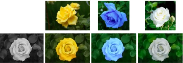
Example-based colorization algorithms are fully automatic. In addition to a target grayscale image to be colorized, they also take as input a color image called the reference image for providing chrominance information. It is necessary to assume that similar contents between the reference image and the target image should have similar chrominance. The third type of method is also automatic, but instead of taking a single reference image, a large number of training images are required as input (e.g. [4]) or else some form of semantic labels (e.g. [5]). Our method belongs to the second type and takes a single reference image as input. It has the advantage that user effort is minimized whilst still providing the user with certain control of the colorization by choosing a suitable reference image. An example is shown in Fig. 1 where different reference images are used to produce different yet meaningful colorized images. Note that only the chrominance information is transferred and the colorized images always keep the same luminance as the input.

Example-based colorization methods are typically com-posed of two steps: chrominance matching and color prop-agation. The chrominance information of the target image is provided by the similarities of pixels or patches in the luminance channel. However, existing methods process each pixel or patch in isolation, and thus suffer from inconsistent chrominance values due to matching errors. Such methods thus resort to color propagation as a post-processing step to improve the results. However, this is unlikely to correct all the matching errors in such a late stage which result in artifacts in the final results. Instead of matching patches (or features) directly, our method builds on an effective sparse pursuit representation. For efficiency and robustness, our method operates at the superpixel level. We extract low, mid and high level features for each superpixel, which are then concatenated to form its descriptor. The collection of feature vectors for all the superpixels from the reference image comprises the dictionary. We formulate colorization of target superpixels as a dictionary-based sparse reconstruction problem. Inspired by the observation that superpixels with similar spatial location and/or feature representation are likely to match close regions from the reference image, we further introduce into the energy formulation a regularization term which promotes locality and

Fig. 1. Image colorization using our method. By using different reference images (top row), the same input grayscale image (bottom left) is effectively colorized to have different yet meaningful colors (bottom row).

substantially improves the matching consistency and coloriza-tion results.

As post-processing, existing methods typically use a color propagation step to eliminate block effects and provide a smooth color image. The widely used least squares diffusion method [3] usually results in an oversmooth image with blurred edges. In [6], the variational based diffusion method is proposed, which involves a total variation (TV) regularization. However, the optimization in [6] only involves the chromi-nance channels, with no coupling of the chromichromi-nance channels with the luminance, which leads to halo effects near strong contours. Furthermore, such propagation methods only depend on the chrominance information of the matching result image, which is often prone to matching errors and poor edge struc-ture. As a result, such propagation methods cannot guarantee the correct edge structure in the final results either. For image colorization, the given target grayscale image is accurate and provides plenty of structure information. We thus propose a novel efficient luminance image guided joint filter to propagate the chrominance information while preserving accurate edges. Although recent work [7] also considers coupling the channels of luminance and chrominance in TV-based regularization to preserve image contours during colorization, the regularization is incorporated in a variational optimization framework which for each pixel selects the best color among a set of color candidates. It still suffers from artifacts of color inconsistency, because locality consistency is not taken into account in the process of choosing color candidates, and it is not possible to resolve this with a variational framework if none of the color candidates are suitable.

Compared with existing work, the main contributions of this paper include:

1) We propose a novel locality consistent sparse repre-sentation for chrominance matching and transfer, which improves the matching consistency dramatically. To our best knowledge, it is the first work that uses dictionary-based sparse representation for colorization using a single reference image, and the first method that ex-ploits locality consistency in the chrominance matching process.

2) We develop a luminance guided joint filter for chromi-nance channel to produce coherent colorized images while preserving accurate edge structure.

Experimental results demonstrate that our colorization method outperforms state-of-the-art methods, both visually and in quantitative analysis of standard measures and a user

study. We review the most relevant research in Sec. II and present the algorithm in Sec. III. We show experimental results in Sec. IV and finally draw conclusions in Sec. V.

II. RELATED WORK

A pioneering semi-automatic scribble based image coloriza-tion method was proposed by Levin et al. [3]. It requires a user to mark color scribbles on the target image, and then applies color propagation based on least squares approximation of linear combination of neighborhood. In order to reduce the color bleeding effects at edges, Huang et al. [8] proposed an adaptive edge detection based colorization algorithm. In [9], a new colorization technique based on salient contours was proposed to reduce color bleeding artifacts caused by weak object boundaries. Yatziv et al.[10] proposed a fast colorization method based on the geodesic distance weighted chrominance blending. In [11], the scribbles are automatically generated to reduce the burden of users, although the color for each scribble still needs to be manually specified. The colorization is con-ducted by quaternion wavelets along equalphase lines. Similar to scribbles, some methods use a sparse set of reference color points on the target image to guide colorization [12], [13]. The sparse representation was first used for image colorization in [14]. Their method however requires as input a large set of training color images to learn a color dictionary, as well as a small subset of color pixels on the target image. Colorization is formulated as a sparse reconstruction problem that uses patches from the dictionary to approximate the target grayscale image as well as the specified color pixels. The method directly works in the color space and thus requires a large training set to sufficiently cover the variation of target images. In addition, image colorization with scribbles can also be seen as a matrix completion problem [15]–[17]. A small portion of accurate chrominance values are required, and then rank regularization is used to guide the color propagation.

Example-based automatic colorization methods do not re-quire user interaction. In this class of algorithms, only a reference image with chrominance information is needed as input, and the target monochrome image is colorized automat-ically. It gives the user some flexible control to help overcome unavoidable semantic ambiguity by providing a suitable image. For example, leaves in an image may be green for spring, or yellow for autumn. Flowers may have a variety of colors such as yellow, blue or white (cf. Fig. 1). Most of the example-based colorization algorithms are motivated by the original work [18] by Welsh et al. For each pixel in the grayscale image, the best matching sample in the color image is found using neighborhood statistics. Then the chrominance values are transferred to the target grayscale image from the color reference image. In order to improve the accuracy of color matching, manual swatches are also defined in [18] to restrict where to search patches in the reference image. Since each pixel is matched in isolation, these methods suffer from color inconsistencies. In order to enhance color consistency, Irony et al. [19] assign the matching color with high confidence as the scribble and propagate the chrominance channel by least squares optimization [3]. Charpiat et al. [20] proposed a global

Luminance guided

joint filter

Locality consistent sparse matching Reference Image

*

…

Target Image

Segmentation and feature extraction

Segmentation and feature extraction

Sparse coefficients Chrominance matching result

Features from target image Dictionary: Features from reference image

…

superpixels

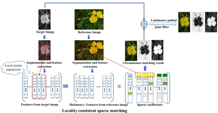
Fig. 2. The pipeline of the proposed colorization algorithm.

optimization method based on graph cut for automatic color assignment. Pang et al. [21] adopted self-similarity to enhance color consistency. In [22] a novel colorization method based on histogram regression was proposed. It assumes that the final colorized image should have a similar color distribution as the reference image, and color matching is conducted by finding and adjusting the zero-points of the color histogram. While enhancing the consistency of colorization, these methods do not however take the structural information of the target image into account, which leads to the blending edge effect. Gupta et al. [23] proposed a cascaded feature matching scheme to automatically find correspondences between superpixels of the reference and target images. An image space voting framework was proposed to improve spatial coherence for the results of initial color assignments derived from superpixel matching. However, locality consistency was not taken into account in the process of superpixel matching. Arbelot et al. [24] proposed a method for both colorization and color transfer. Based on the region covariance texture descriptor, they introduced a new multi-scale gradient descent optimization, and unnormalized bilateral filtering to improve the edge-awareness of feature descriptors, leading to improved results, especially near region boundaries. Incorrect matching may still exist if different regions have similar texture descriptors. In [6], a variational image colorization algorithm was proposed. For each pixel, some candidate matchings are given, and an optimization involving an edge-preserving total variation is used to choose the best matching. The work in [25] generalized the variational method to RGB space to ensure better color consistency. In order to eliminate halo effects near strong contours, [7] intro-duced a coupled regularization term with luminance channel to preserve image contours during the colorization process. Instead of using a static combination of multiple features to

improve the matching performance, [26] proposed an auto-matic feature selection based image colorization method via a Markov Random Field (MRF) model.

Our method also takes a single color image as reference. Unlike existing approaches, we formulate target colorization as an effective sparse pursuit dictionary-based formulation, where the dictionary is built using features from the reference image. We further introduce locality consistency regularization in the optimization framework to find consistent chrominance information for the target image. By incorporating locali-ty consistency in the matching stage rather than in post-processing as existing methods did, it substantially improves color consistency and reduces artifacts. This is further im-proved by a new edge preserving luminance-guided joint filter, which leads to significantly better results than existing methods.

Other methods for colorization use different types of input. Liu et al. [27] firstly recover an illumination-independent intrinsic reflectance image of the target scene from multi-ple color reference images obtained by Internet search, and then transfer color from the color reflectance images to the grayscale reflectance image while preserving the illumination component of the target image. The method is mainly de-signed for landmark scenes where Internet images are widely available and can be easily retrieved. Chia et al. [5] require a pre-segmented target image with semantic labels and search within Internet images with associated semantic labels to colorize the target image. The method is also generalized to semantic portrait color transfer [28]. Deshpande et al. [29] propose an automated method for image colorization that learns colorization from a set of examples (rather than one reference image) by exploiting the LEARCH (learning-to-search) framework. Wang et al. [30] colorize images based on

affective words. Recently, deep learning based methods have been proposed to colorize a given grayscale image [4], [31]– [33]. After training, the method only needs target grayscale images as input, although a large set of images are needed for training to cover the variation of target images. It is also unclear how semantic ambiguities (e.g. leaves of different colors) can be resolved. Image colorization is also related to color transfer where the target image is a color image and the purpose is to change its color style (e.g. [34]–[38]). A similar problem is color harmonization where the style of color image is enhanced to improve aesthetics [39], [40].

III. IMAGE COLORIZATION BY LOCALITY CONSISTENT SPARSE REPRESENTATION

The pipeline of the proposed algorithm is shown in Fig. 2. Firstly, we apply global linear luminance remapping to the reference image such that the resulting image has the same luminance mean and standard deviation as the target, which helps suppress the influence of global luminance difference between the two images, as in [18]. Then both the reference and target images are segmented into superpixels, and features are extracted from each superpixel. The features from the reference image comprise the dictionary, and each feature from the target image should be sparsely represented by a few elements of the dictionary. To enhance color consistency, a locality consistent sparse representation learning method is used that encourages matches for local similar superpixels in the target image to come from neighboring superpixels in the reference image. With the assumption that pixels with similar structure should have similar color, the chrominance information is transferred to the target image via sparse matching. The obtained color image however may still contain some mismatching and incorrect edge information, so we further develop an edge-preserving propagation process for the chrominance channel with the guidance of luminance information of the target image. Finally, the luminance channel and the chrominance channels compose the final colorization result of the target grayscale image.

A. Superpixel segmentation and feature extraction

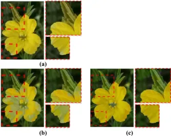
1) Superpixel segmentation: At the first step, we segment both the reference image and the target grayscale image into superpixels. For the reference image, superpixel segmentation is conducted using the color information in the reference image. The target grayscale image is segmented using the luminance information. Doing so maximizes the use of in-formation and ensures uniformity within each superpixel. We adopt the Turbopixel algorithm [41], which can process color and grayscale images while preserving the edge structure well. The parameters are set as the default values in the source code1. Fig. 3 shows the superpixel segmentation results for the color and grayscale images. From the magnified selection of the boundary area, we can see that the edge information is well preserved.

1_{http://www.cs.toronto.edu/˜babalex}

Fig. 3. Superpixel segmentation results. From the zoomed in window, it can be seen that the edge is well preserved after superpixel segmentation.

2) Feature extraction: For each superpixel, features from different levels are extracted to form its descriptor. For both the reference image and target image, the features are extracted only from the luminance channel to make them comparable. We use a combination of low, mid and high level features to cover a wide range of characteristics. We choose features to be robust, distinctive and efficient to compute. The low level intensity-based features include mean value, standard deviation, the local contrast and the histogram of intensity. A local image textural descriptor DAISY [42] composes the mid-level feature, and the saliency value of each superpixel is regarded as the high-level semantic feature.

Low-level feature. A 28-dimensional feature vector is computed for each superpixelSibased on the intensity values.

The first two componentsfl

1(i)andf2l(i)for the ith

super-pixel are the mean and standard deviation of the intensities of pixels in the superpixel, with the pixel intensity represented as a number between 0 (black) and 1 (white). The third dimension fl

3(i)is the local contrast. It measures the uniqueness of

su-perpixel intensity compared with its neighboring susu-perpixels: f3l(i) = X Sj∈N(Si) ω(p_i,p_j) f1l(i)−f1l(j) 2 ,

where N(Si) is the neighborhood of superpixel Si, which

is set to the 8 nearest superpixels (measured based on the Euclidean distance between the centers of superpixels) in all the experiments. Since the number of directly adjacent super-pixels can vary significantly, using geometric closeness is more robust than using adjacent superpixels.pirepresents the spatial

location of the center of superpixelSi, with each coordinate

normalized to [0,1]. ω(pi,pj) = exp −(pi−pj)2/σ2 is

the local weight function.σ= 0.25is used in our experiments. If the distance between superpixelsSj andSi is smaller, the

weight will be larger, leading to a more significant contribution to the contrast measure (Fig. 4(d)).

The last component fl

4(i) is a histogram of the intensity

distribution within each superpixel. In our experiments, the intensity range 0–1 is divided into 25 bins, and each entry represents the ratio between the number of pixels with the intensity belonging to the bin and the total number of pixels in the superpixel.

These four types of features are then concatenated to form the low-level feature fl _={fl

fl

4 is 25 dimensional, its entries are summed to 1, which

makes this component have a comparable contribution to other components.

Mid-level feature. Intensity-based low level features is effective at distinguishing regions with significant difference in intensity or their statistics, but performs worse for highly textured regions as the texture structure cannot be effectively captured. We resort to mid-level local texture features for this purpose. We use DAISY [42] as the mid-level feature, which is a fast local descriptor for dense matching. While retaining the robustness to rotation, transition and scaling similar to descriptors such as SIFT (Scale-Invariant Feature Transform) and GLOH (Gradient Location and Orientation Histogram), it can be calculated much faster. For each pixel, DAISY creates a 25×8 dimensional matrix descriptor, with each row as a normalized histogram. We reshape it to form a 200

dimensional vector feature, and further reduce the dimension to 25 using PCA (Principal Component Analysis), to make the later dictionary-based sparse representation more efficient, while keeping the comparable visual quality. The DAISY feature is normalized to have entries summed to 1. The mid-level texture feature is denoted as fm_.

High-level feature. Image saliency is used to model human attention in images, which is a higher-level semantic feature compared with intensity and textures (Fig. 4(e)). For the task of image colorization, the reference image and target image generally have similar structure, so for example the salient regions in the target image should be expected to match the candidates from high saliency regions of the reference image. The constraint of saliency is thus effective to ensure semantic consistency. In this paper, we use the saliency detection method [43] due to its robustness. The high-level saliency feature is denoted as fh_.

In order to make each feature have a comparable contribu-tion over all three levels, features containing single values are normalized to the range of[0−1], and vector-based features are normalized with a sum of 1.

B. Chrominance transfer by locality consistent sparse match-ing

In this paper, we formulate the superpixel matching problem as a sparse representation problem. The collection of features for superpixels from the reference image composes the dictio-naryR={f_Ri, i= 1,2,· · ·, M}, wheref_Ri = (fl Ri,f m Ri, f h Ri)

is the feature of the ith _{superpixel from the reference image}

and M is the total number of superpixels in the reference image. For each feature vector of the superpixel from the target grayscale image, its featuref_Tj = (fl

Tj,f m Tj, f

h

Tj)should

be sparsely represented by this dictionary with the assump-tion that the reference image and the target image should contain semantically similar objects. Then the chrominance information of the target image can be transferred from the corresponding superpixels in the reference image.

The general sparse representation [44] commonly used in subspace clustering assumes that a data point drawn from the union of multiple subspaces admits a sparse representation with respect to the dictionary formed by all other data points.

(a) (b) (c) (d) (e)

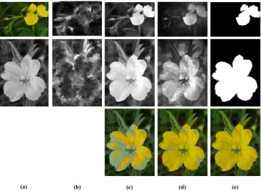
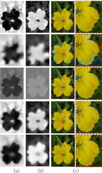
Fig. 4. Demonstration of different features and their contribution to colorization. (a) reference and target images, (b-e): from left to right, different features with the first two rows visualizing the features for reference and target images, and the last row showing the color matching results with corresponding features added. The mid-level DAISY feature is included by default, as well as the features previously added. (b) standard deviation, (c) mean, (d) local contrast, (e) saliency.

Fig. 5. Comparison between the traditional sparse method using isolated matching and the proposed locality consistent sparse matching.

In the noiseless case, the sparse coefficients can be found by solving the following ℓ1 optimization problem.

min

α

kαk₁, s.t.f_T =Rα, (1)

where f_T = {f_Tj} is a matrix collecting all the feature vectors of target superpixels and α is the matrix containing

coefficients for reconstructing f_T using feature vectors in the dictionary R. Sparse representation methods have achieved state-of-the-art results in a variety of applications. However, general sparse representation only focuses on pursuing the linear correlation of data. It does not take into account the local manifold structure of data, and hence if several data points have strong linear correlation with the given data, it will randomly choose one. In addition, a general sparse representa-tion processes data in isolarepresenta-tion, ignoring locality consistency, as illustrated in Fig. 5. For the task of image colorization, numerous isolated error matching will be introduced by using the general sparse method (see Fig. 6(a)). For example, some superpixels of the yellow flower are mismatched to a green leaf even if their neighboring superpixels are correctly matched. An intuitive approach to improving the matching accuracy is to

utilize the local structure of data. In this example, neighboring superpixels of the flower with similar features should be matched consistently.

Based on the above motivation, we propose a locality consistent sparsematching algorithm. We first define a locality structure consistency measurewij between two superpixelsSi

and Sj. Two criteria are involved: (i) two superpixels with

small spatial distance should have similar matching results with high probability; (ii) superpixels which are close in feature space should have similar matching results. Based on the above analysis, the local consistency measure is defined as follows, similar to bilateral filtering:

wij = exp ( −kpi−pjk 2 σ2 1 ) exp ( −kfi−fjk 2 σ2 2 ) , (2) where p_i is the spatial location of the center of the ith

superpixel, andf_i is the feature of theith superpixel.σ1 and

σ2are scaling parameters for the spatial and feature measures

(see Section IV for detailed discussion about their choices).

W={wij}measures the local consistency of superpixels.wij

is larger when two superpixels are closer in spatial location and in the feature space.

Finally, the locality consistent sparse matching model is formulated as: min Z kfT −RZk 2_+λX i,j wijkZi−Zjk2+βkZk1, (3)

whereZcontains reconstruction coefficients, andZi is theith

column ofZ with coefficients representing the ith _superpixel

of the target image.

The first term is the data-fidelity constraint, which ensures accurate reconstruction using the global linear representation. The second term is the new locality consistent regularization. When two superpixels are similar, wij is large. In this

sit-uation, kZi−Zjk needs to be small in order to minimize

the energy. Therefore, the matching results will be provided with high locality consistency by this term. The third term is the sparse regularization, which ensures that each target superpixel should only be represented by a small number of candidates in the reference image, which promotesuniqueness

of the matching results to avoid ambiguity in chrominance transfer.

Fig. 6 compares chrominance transfer results of the pro-posed locality consistent sparse matching method against two alternative isolated matching methods. Fig. 6(a) shows the result of the isolated cascaded matching method used in [23], and Fig. 6(b) is the result obtained using the general sparse representation model (Eqn. (1)). It can be seen that in both (a) and (b), some superpixels of the yellow flower are mismatched to green leaves even if their neighboring superpixels are cor-rectly matched. By using our locality consistent regularization (Eqn. (3)), the matching accuracy in Fig. 6(c) is substantially improved.

C. Optimizing the locality consistent sparse model

Minimization of model (3) can be solved efficiently by the alternating direction method of multipliers (ADMM) algorith-m [45]. In order to algorith-make the problealgorith-m separable, an extra

(a)

(b) (c)

Fig. 6. Demonstration of chrominance transfer results with (a) isolated matching by [23], (b) isolated sparse representation (Eqn. 1) and (c) our proposed locality consistent sparse representation (Eqn. 3).

variable P is introduced, and the original model (3) can be rewritten as follows in the matrix form:

min

Z,PkfT −RZk

2_+λ·tr(ZLZT_{) +βkPk}

1, s.t.Z=P,

where tr(·) is the trace of a matrix, which equals the sum of the diagonal elements. L = D−W is the Laplacian matrix of W, where D is the degree matrix of W, i.e.

D=diag(di), di =Pjwij. Using the method of Lagrange

multipliers gives the following equation:

min Z,PkfT −RZk 2_+λ·tr(ZLZT_{) +βkPk} 1 +γ 2kZ−Pk 2_+<τ,Z−P>,

whereτ is the Lagrange multiplier. Then the variablesZand

Pwill be updated in an alternating fashion.

When P is fixed, Z can be solved by the following differentiable optimization: min Z kfT −RZk 2_+λ·tr(ZLZT_{) +}γ 2kZ−P+ τ γk 2 (4) Given thekth _iterationPk _andτk_{, the optimalZfor Eqn. (4)}

is obtained by solving the following Sylvester equation

(γ−2RTR)Zk+1+λZk+1(LT +L) + 2RTfT

−γ(Pk−τ

k

γ ) = 0. (5)

For fixed Z, the optimalPcan be solved by optimizing

min P kPk1+ γ 2βkP−Z− τ γk 2_. (6) The problem (6) has a closed form solution, which can be solved by the following soft-thresholding operator

Pk+1=Sβ γ( Zk+1+τ k γ ), (7) where Sλ(v) =      v−λ, ifv≥λ 0, if|v|< λ v+λ, ifv≤ −λ

(a) (b)

(c) (d)

Fig. 7. Comparison of image filtering results on synthetic data. (a) luminance image (l), (b) initial chrominance image u0, (c) result of least squares

filtering (Eqn. 8), (d) our luminance guided joint filtering result.

Finally, the Lagrangian multiplier τ will be updated by τk+1 = τk+γ(Zk+1−Pk+1). This process repeats until

convergence. The pseudocode is provided in Algorithm 1. The parameters are set as follows: λ= 0.1,β = 1 and tolerance ε= 10−6. These are fixed for all the experiments.

Algorithm 1 The ADMM solution for optimizing (3).

Input:

DictionaryR, the features of target imagefT.

1: Initialize: P=0

2: repeat

3: For fixedP, solve Zby the Sylvester equation (5) 4: For fixed Z, solve P by the singular value shrinkage

operator (7);

5: Update the Lagrange multipliers: τk+1 = τk +

γ(Zk+1_−Pk+1₎

6: untilkf_T−RZk∞< εandkZ−Pk∞< ε Output: Return the optimal solution{Z∗}

After solving the locality consistent sparse problem, the chrominance information of the jth _{superpixel in the target}

image will be transferred from the corresponding chrominance channel of the dominant superpixel in the reference image (the superpixel with the largest representation coefficient), i.e. uTj = uSi, where i = arg maxk(Zj(k)), u represents a

chrominance channel, anduSi is the mean chrominance value

of thei-th superpixel in the reference image. We use the YUV color space in this paper, where uhere refers to the U and V chrominance channels respectively.

D. Edge-preserving joint filtering guided by luminance

Although the locality consistent sparse matching dramati-cally improves color transfer results, matching errors may still exist. In particular, as the chrominance channels are transferred on a superpixel basis, the resulting chrominance images show strong block effects and can have quite a few sparse outliers,

(a)

(b)

(c)

Fig. 8. Effect of edge-preserving joint filter. (a) U chrominance channel, (b) V chrominance channel (c) color image. The first row is the matching result, and from the second row to the last row are respectively the results of least-squares filtering (Eqn. 8), guided image filtering [46], joint bilateral filtering [47] used in [4], and our proposed luminance guided joint filtering

(Eqn. 9) _.

as shown in Fig. 8. In this section, we will develop a new luminance guided joint filter for the chrominance channel to achieve consistent chrominance images whilst preserving the edge information.

Most of the existing colorization methods use the following weighted least squares optimization [3] to propagate color information: min u X i (ui− X j∈N(i) ˜ wijuj)2 (8)

where w˜ij is the similarity measure between pixels i and j.

However, the model (8) is an optimized low-pass filter. It can smooth the block effect but also causes the edges to be blurred, as shown in the second row of Fig. 8. Moreover, this class of methods only uses the information of the chrominance image, which inevitably contains matching errors and poor edge

structures, making reliable propagation challenging. For image colorization, the given target grayscale image is assumed to be accurate and provides reliable structure information. Therefore, we propose to exploit the target grayscale image explicitly as guidance for the propagation of chrominance information.

In this paper, we propose a new joint filter for chromi-nance images guided by the lumichromi-nance images. One of the most important criteria for propagation is that the filtered chrominance image should preserve the edge structure well. However, the chrominance images obtained by direct matching in the previous step often fail to preserve the edges and may even introduce wrong edges. In this situation, the given target luminance image can provide accurate guidance. Based on the analysis above, such luminance guided chrominance channel filtering can be formulated as an optimization problem, with the optimization of both chrominance channels separable. As a result, we filter each chrominance channel individually, and the designed filter for each chrominance channel can be written as follows: min u E(u) = Z k (uk−u0k) 2_{+ηk∇u− ∇lk}2_dk (9) where k integrates over the whole image, u is the filtered chrominance image,u0is the chrominance image from sparse

matching, l is the given target luminance image, and ∇· is the gradient operator. The first term of equation (9) is the data fidelity term, and the second term is the gradient regularization with the guidance of the luminance image, which ensures accurate edge structure of the output chrominance image.

The optimaluthat minimizes this energy satisfies the Euler-Lagrange equation: ∂E ∂u − ∂ ∂x ∂E ∂ux − ∂ ∂y ∂E ∂uy = 0,

where ux = ∂u_∂x and uy = ∂u_∂y are the chrominance gradient

w.r.t.xandy. By substituting and differentiating, we have the following

u−η∇2_u=u

0−η∇2l. (10)

This is a typical 2D screened Poisson equation which has been discussed in [48], and it can be solved efficiently in the Fourier domain.

In order to evaluate the effectiveness of the proposed joint filter, we design a simple synthetic experiment. Fig. 7(a) is the original imagel∈R200×200of which the top half is0(black) and the bottom half is1(white). Fig. 7(b) simulates the initial distributionu0with some sample pixels set to different values

(0.5). Figs. 7(c)&(d) are obtained by filtering of the image (b), with weighted least squares (Eqn. 8) and our proposed luminance guided approach (Eqn. 9). It can be seen that the weighted least squares model produces an overly smoothed result and loses the edge structure whereas the joint filter proposed in this paper preserves the edge structure well with the guidance of the original image l.

We also evaluate the performance of the luminance guided joint filter on a real colorization example (see Fig. 8). For a thorough evaluation, we also compare our luminance guided joint filtering with the joint bilateral filtering [47] used in

recent colorization work [4], and guided image filtering [46]. Guided image filtering [46] is well known for improved structure preservation by using a guidance image and a locally adaptive linear model. We use the target grayscale image to guide the filtering of the chrominance images as [26] does. Fig. 8 compares the filtering results. With our joint filter (fifth row), the chrominance image has better consistency in uniform regions and preserves the edge structure well, whereas the least squares propagation result has an obvious blur effect around the edge (second row), causing color bleeding. The guided filter can also keep the edge sharp, but the detailed texture is overly smoothed (see the third row). Although the joint bilateral filtering [47] itself is anisotropic, individual Gaussian weighting functions are isotropic, and thus it would produce halo effects along salient edges. Perceptually, this leads to the final images losing some sharpness and having some ‘feathering’ artifacts around edges (see the fourth row). We also visualize the pixel distribution in the YUV color space in Fig. 9. It can be seen that the filtered results by least squares propagation (b), guided image filter (c) and joint bilateral filter (d) produce many colors not present in the reference image, while our proposed joint filter result (e) has a very similar distribution as the reference (a).

We summarize the overall locality consistent image col-orization algorithm in Algorithm 2. After superpixel segmen-tation and feature extraction, we use the locality consistent sparse matching to transfer the chrominance channels from the reference image to the target image (denoted as u0 and

v0). These chrominance images are further refined using the

luminance guided joint filter to produce improved chrominance images u and v. The final colorization image is obtained by combining the given target grayscale image with the chrominance imagesuandv.

Algorithm 2Image colorization by locality consistent sparse representation.

Input:

A color reference image R, a grayscale target image T. 1: Superpixel segmentation and feature extraction,

calculat-ing fR,fT, and the dictionaryR={fR} ;

2: Chrominance transfer by locality consistent sparse match-ing (Eqn. 3) to obtain the initial chrominance images u0

andv0;

3: Edge-preserving luminance guided joint filter (Eqn. 9) to produce the final chrominance images uandv;

Output: Return the colorized image TC by combining the

luminance imagel with the chrominance imagesuandv.

IV. EXPERIMENTALRESULTS

In this section, we present experimental results to evaluate the influence of different parameter settings, compare the performance against several state-of-the-art methods using extensive examples, along with a user study for quantitative evaluation of subjective user preferences. Finally we extend our method to color transfer.

(a)

(b)

(c)

Pixels in YUV Space

80 60 Y 40 20 0 80 70 60 50 40 30 20 10 0 V

(d)

(e)

Fig. 9. Pixel distribution in the YUV color space. (a-e): visualization of pixel distribution of the reference color image and the propagation results (second to fifth rows of Fig. 8). Compared with the original distribution as shown in (a), the color distribution generated by our proposed method (e) is very similar, whereas the least squares filtering (b), guided image filtering (c) and joint bilateral filtering (d) produce significant numbers of pixels with unrelated colors.

(a) (b)

(c) (d) (e)

Fig. 10. The influence of parametersσ1 andσ2 using extreme values. (a)

reference image, (b) target image, (c-e) sparse matching results corresponding to different parameters. (c)σ1 = 10−6,σ2= 1. (d)σ1 = 10,σ2= 1. (e)

σ1= 106,σ2= 1.

A. Parameter settings

There are 3 parameters key to the performance of the proposed algorithm. The first two parameters are σ1 and σ2

in the locality weighting function (Eqn. 5), and the third parameter is η in the edge-preserving joint filter (Eqn. 11). We analyze their effect by varying these parameters.

σ1controls the spatial locality, whileσ2controls the feature

similarity. As an extreme case, Fig. 10 shows the color matching results with σ2 fixed at 1 andσ1 adjusted to10−6,

10 and 106_{, respectively. When σ}

1 is close to 0, the weight W defined in Eqn. 2 will be close to 0, which means the locality consistency term in Eqn. 3 is almost ignored. Fig. 10 (c) shows that many mismatches occur without this term, e.g.,

(a) (b) (c) Ground truth

Fig. 11. The influence of edge-preserving parameterηto the filtering result with Fig. 10(d) as input. The first row shows the results withη= 10−5_,0_.05

and the ground truth image, the second and third rows present color distribu-tion using a 2-D color scatter diagram and a 1-D color histogram.

some patches of flowers are mismatched to the blue sky. On the other hand, whenσ1 is too big, the spatial consistency in

(Eqn. 2) will be fixed to a constant1for every superpixel, and the locality consistency term will be determined entirely by the feature similarity. Fig. 10 (e) shows that some isolated matches occur without the spatial constraint. Fig. 10 (d) reports the best performance with suitable parameters that enable both spatial and feature consistency. Note that these are sparse matching results, which will be further improved by our joint filtering.

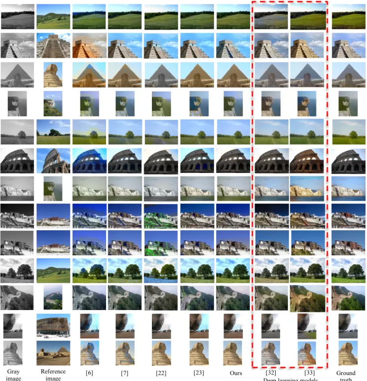
[22]

[6] [7] [23] Ours

Deep learning models

[32] [33] Ground truth Gray image Reference image

Fig. 12. Comparison of our colorization results with alternative methods.

The parameter η in the luminance guided joint filtering (Eqn. 9) controls the effect of edge-preserving. We evaluate the effect of varyingηbased on the matching result in Fig. 10 (d) where σ1= 10, σ2= 1 are used. The propagation results

with varying ηare shown in the first row of Fig. 11. It can be seen that small η results in oversmoothing and edge blending effect. The smaller the value ofη, the weaker the preservation of the edges. η = 0.05is a good choice for most images. In order to evaluate the propagation performance intuitively, we visualize it using the 1-D color histogram (third row) and

2-D color scatter diagram (second row). From the 1-2-D and 2-2-D color distributions, we can see that whenη= 10−5_{, the results}

have obvious color distortion with respect to the ground truth image. Comparatively, whenη= 0.05the color distribution is very similar to that of the ground truth image, which implies faithful color transfer.

For the rest of experiments, the parameters are set asσ1=

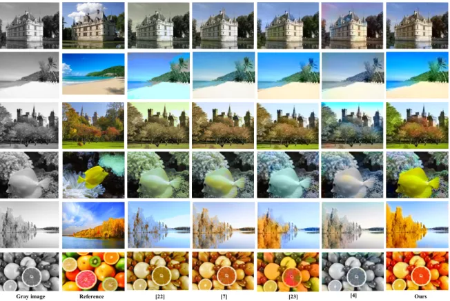
Reference [22] [7]

Gray image [23] [4] Ours

Fig. 13. Comparison of our colorization results with alternative state-of-the-art colorization methods.

B. Visual inspection

In this section, we compare the colorization results of our method against state-of-the-art methods [6], [7], [22], [23], [32], [33] for automatic colorization. The first four method-s [6], [7], [22], [23] are example-bamethod-sed colorization methodmethod-s, which only take one reference image with chrominance infor-mation to provide color for the target grayscale image, whereas methods [32], [33] are deep learning based, which exploit a huge number of images for training their models and do not take reference images into account. In order to make a fair comparison, the results of algorithm [22], [23], [32], [33] are generated by the code provided by the authors, and the results of [6] and [7] are provided by the corresponding authors.

As there is no benchmark for image colorization, we e-valuate different algorithms on natural images which cover a wide variety of image types. Some experimental results are shown in Fig. 12. Both [6] and [7] treat image colorization as a problem of automatically selecting the best color among a set of color candidates. In order to keep the structure information, such as edges and color consistency, a total variation based framework is proposed. [6] only retains the U and V channels, and there is no coupling of the chrominance channels with the luminance, which leads to halo effects near strong contours in their regularization algorithm (see e.g. the second and third rows of Fig. 12). In [7], a strong regularization by coupling the channels of luminance and chrominance is proposed to preserve image contours during colorization. However, for both methods [6] and [7], locality consistency is not taken into account in the process of choosing color candidates. Thus their results still contain artifacts of color inconsistency (see

examples in Fig. 12). The method [22] is a global matching algorithm. The luminance-color correspondence is found by finding and adjusting the zero-points of the histogram. It is automatic and efficient, and can get satisfactory performance when the image has strong contrast. However, due to its global mechanism, when the zero-points based correspondence has some error, it will result in many mismatches, as shown in the 8th-11th rows of Fig. 12. Furthermore the method [22] does not take into account structure preservation, resulting in visible color blending (e.g. the 4th row of Fig. 12). The method [23] similarly employs isolated cascaded matching. They then develop an explicit voting scheme for color assignment after the matching step to improve results. However, the isolated color mismatches still remain in the colorization results. For example, in the 11th row of Fig. 12, part of the wall is mismatched to the green leaves while its neighboring regions are colorized correctly. In comparison, locality consistency is significantly enhanced in our color matching process, and the colorization results are further improved by our luminance guided propagation. It can be seen from visual inspection of Fig. 12 that our algorithm achieves best performance, even for challenging cases with similar textures where existing methods fail to produce satisfactory results.

In addition to example-based methods, we also compare our colorization results against the latest deep-learning based methods [32], [33]. In general, they can generate reasonable colorized images, as shown in Fig. 12. However, there are still some obvious artifacts shown e.g. in the first row where part of the meadow is colorized in blue by [32] and in the last row where part of the pyramid is colorized in blue by

[33]. In addition, the output of such deep learning based methods cannot be controlled by the user, unlike example based methods.

Some colorization results for scenes with complex structure and large color variation are shown in Fig. 13. These examples are more challenging, as regions with substantially different colors can have similar local characteristics in grayscale im-ages. We compare our results with state-of-the-art colorization methods based on global and local matching as well as deep learning2_{. The method [22] is a global matching algorithm. For} such examples, the method does not reproduce the original colors from the reference images. For example, the method generates a colorless output for the example in the 1st row, and outputs images with a uniform blended color in the 3rd to 6th rows. For the example in the 2nd row, it colorizes the beach wrongly in turquoise, and produces large color patches with clear boundaries in the sky. The methods [7], [23] are based on local matching. For the example in the 1st row, compared with [7], [23], our result avoids the green tint on the building which does not appear in the reference image, and reproduces green color in the water as in the reference image. For the example in the 2nd row, the result of [7] has an overall blue tone in the result, with the plants and shadow looking blue, and sand appearing pale compared with the original color, whereas both our method and [23] produce output images with plausible colors. For the example in the 3rd row, the results of both [7] and [23] are significantly less colorful than the reference image. Our result effectively transfers the color from the reference image and produces a reasonable colorful output. The examples in the 4th and 5th rows have regions of different colors with similar textures. Thus the results of [7], [23] tend to either mix different colors, leading to a bland looking output (e.g. the fish example of [23]) or have patchy output using colors from different regions (e.g. the fish example of [7]). Our method produces better results overall. For the example in the 6th row, our method effectively colorizes a variety of fruits in suitable colors. Note that although the reference image contains limes (in green) and oranges (in yellow/orange), they look very similar in the grayscale image. As a result, our result colorizes fruits in yellow/orange rather than green, based on matching. While being plausible, it would be better if objects can be matched more accurately. This is a limitation of our current approach. Nevertheless, our locality consistent matching produces coherent colorization for objects, and avoids color inconsistencies (e.g. the grapefruit) in the results of [7], [23]. Our colorization result shows some color reflection (e.g. an orange adjacent to a red fruit has red tint reflected). This is in fact correct, as can be seen from the subtle hints in the grayscale target image (highlight and grayscale level change corresponding to reflection). We also present results of these examples with a state-of-the-art deep learning based method [4] using the code with a pre-trained model provided by the authors3_{. Different from our method, this} method does not require reference images and only takes target

2_{For this example, we compare with methods where code is publicly}

available, so the result of [6] is not included.

3_{http://cs.sjtu.edu.cn/shengbin/colorization/}

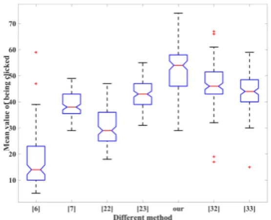
Fig. 14. Boxplots of user preferences for different methods, showing the mean (red line), quartiles, and extremes (black lines) of the distributions.

grayscale images as input. The results are not very colorful and contain some unreasonable colors. This may be because these examples are significantly different from the images used to train their model.

C. User evaluation

In addition to visual inspection, we would like to also make quantitative comparisons with existing methods. However, it is known that standard signal measures such as the standard Peak Signal to Noise Ratio (PSNR) can deviate substantially from human perceptual differences. Improved methods have been developed for image quality assessment in general, such as Structural SIMilarity (SSIM) [49]. However, such measures are not appropriate for the task of image colorization, e.g. because colorization different from the ground truth may still be perfectly plausible. Therefore, in order to make a fair comparison, we perform a user study to quantitatively evaluate our method against other three methods.

TABLE I

THE P-VALUE OFANOVATEST OF PROPOSED METHOD AGAINST OTHER METHODS.

method [6] [7] [22] [23] [32] [33] p-value 6.51e-74 1.47e-32 2.18e-56 4.20e-18 1.51e-06 2.95e-13 The user study is designed using the 2AFC (Two-Alternative Forced Choice) paradigm, widely used in psychological stud-ies due to its simplicity and reliability. To make the comparison more meaningful while limiting the user effort to a reasonable level, we use the full set of results in Fig. 12 containing 13 test images and colorization results generated by seven methods ([6], [7], [22], [23], [32], [33] and our method). The detailed user study results are given in the supplementary material. 120 users participated in the user study, with ages ranging from 18 to 60. For each test image, every pair of results is shown and the user is asked to choose the one of them that looks better. To make sure deep learning based methods are not disadvan-taged, we do not explicitly ask users to evaluate similarity of colorization to the given reference images. To avoid bias, we randomize the order of image pairs shown and their left/right position. Altogether, results of each method are compared against13×6 = 78results of alternative methods. We record

Target Reference Target Reference [35] [36] [37] [34] [38] Ours [35] [36] [37] [34] [38] Ours

Fig. 15. Comparison of color transfer using our method and state-of-the-art example-based methods.

the total number of user preferences (clicks) for each method, and treat these as random variables. The distribution of user preferences for each method is summarized in Fig. 14. The one-way analysis of variance (ANOVA) is used to analyze the user study results. ANOVA is designed to determine whether there are any significant differences between the means of two or more independent (unrelated) groups. It returns the p-value for the null hypothesis that the means of the groups are equal. The smaller the p-value obtained by ANOVA, the more significant the groups are. In this paper, the p-values are computed against each compared method and the results are shown in Table I. We can see that all of the p-values are small (<10−5_{) which implies the judgements of all users on}

different methods are statistically significant. From Fig. 14 we can see that majority of the users prefer the method proposed in this paper which has the highest mean score.

D. Extension to Color Transfer

Color transfer is an application related to colorization, with the aim of altering the color style of a target color

image to match that of a given reference image. The main difference between image colorization and color transfer is that no chrominance information is available for colorization. Although our method is designed for colorization, the pro-posed locality consistency based colorization algorithm can also be generalized to solve the color transfer problem. The overall pipeline is the same, with the following two changes to benefit from the additional color information of the target image: 1) Superpixel segmentation of the target image now uses the full color information, similar to the reference image. This helps to differentiate regions with similar grayscale level but different colors. 2) The feature similarity measure W

in the locality consistent sparse matching now uses all the color channels, instead of just using the grayscale level.

Note that we do not assume the reference and target colors are correlated, but instead the additional color information helps differentiate different content in the target image. Some examples of color transfer using our method are presented in Fig. 15. Compared with state-of-the-art color transfer methods, our method faithfully transfers the color style of the reference to the target, whereas existing methods tend to have visible artifacts of non-smooth pixels and unrelated colors.

V. CONCLUSIONS

In this paper, we propose a new automatic image col-orization method based on two major technical advances, namely locality consistent sparse representation and a new edge-preserving luminance guided joint filter. Extensive exper-iments of individual techniques and the overall system using visual inspection and a user study have shown that our novel method significantly outperforms state-of-the-art methods. Our method is also effectively generalized to color transfer. In the future, we would like extend our method to other color-related applications, such as image harmonization, semantic based image color enhancement, etc.

ACKNOWLEDGEMENTS

We would like to thank the authors of [4], [22], [23], [32], [33] for providing their source code, and the authors of [6] and [7] for providing the colorization results presented in Fig. 12 in the paper. We also want to thank the authors of [34]– [37] for providing the codes for image color transfer. This work is funded by National Natural Science Foundation of China (NSFC) 61262050, 61562062, 61502541, 61370186.

REFERENCES

[1] D. S`ykora, J. Buri´anek, and J. ˇZ´ara, “Colorization of black-and-white cartoons,”Image and Vision Computing, vol. 23, no. 9, pp. 767–782, 2005.

[2] E. S. Gastal and M. M. Oliveira, “Domain transform for edge-aware image and video processing,”ACM Transactions on Graphics, vol. 30, no. 4, p. 69, 2011.

[3] A. Levin, D. Lischinski, and Y. Weiss, “Colorization using optimization,”

ACM Transactions on Graphics, vol. 23, no. 3, pp. 689–694, 2004. [4] Z. Cheng, Q. Yang, and B. Sheng, “Deep colorization,” in IEEE

International Conference on Computer Vision, 2015, pp. 415–423. [5] A. Y.-S. Chia, S. Zhuo, R. K. Gupta, Y.-W. Tai, S.-Y. Cho, P. Tan, and

S. Lin, “Semantic colorization with internet images,”ACM Transactions on Graphics, pp. 156:1–7, 2011.

[6] A. Bugeau, V.-T. Ta, and N. Papadakis, “Variational exemplar-based image colorization,”IEEE Transactions on Image Processing, vol. 23, no. 1, pp. 298–307, 2014.

[7] F. Pierre, J.-F. Aujol, A. Bugeau, N. Papadakis, and V.-T. Ta, “Luminance-chrominance model for image colorization,”SIAM Journal on Imaging Sciences, vol. 8, no. 1, pp. 536–563, 2015.

[8] Y.-C. Huang, Y.-S. Tung, J.-C. Chen, S.-W. Wang, and J.-L. Wu, “An adaptive edge detection based colorization algorithm and its application-s,” inACM Multimedia, 2005, pp. 351–354.

[9] N. Anagnostopoulos, C. Iakovidou, A. Amanatiadis, Y. Boutalis, and S. Chatzichristofis, “Two-staged image colorization based on salient contours,” inIEEE International Conference on Imaging Systems and Techniques, 2014, pp. 381–385.

[10] L. Yatziv and G. Sapiro, “Fast image and video colorization us-ing chrominance blendus-ing,” IEEE Transactions on Image Processing, vol. 15, no. 5, pp. 1120–1129, 2006.

[11] X. Ding, Y. Xu, L. Deng, and X. Yang, “Colorization using quaternion algebra with automatic scribble generation,”Advances in Multimedia Modeling, pp. 103–114, 2012.

[12] H. Noda, M. Niimi, and J. Korekuni, “Simple and efficient colorization in YCbCr color space,” inInternational Conference on Pattern Recog-nition, 2006, pp. 685–688.

[13] D. Nie, Q. Ma, L. Ma, and S. Xiao, “Optimization based grayscale image colorization,”Pattern Recognition Letters, vol. 28, pp. 1445–1451, 2007. [14] J. Pang, O. C. Au, K. Tang, and Y. Guo, “Image colorization using sparse representation,” inIEEE International Conference on Acoustics, Speech and Signal Processing, 2013, pp. 1578–1582.

[15] S. Wang and Z. Zhang, “Colorization by matrix completion,” inAAAI Conference on Artificial Intelligence, 2012, pp. 1169–1175.

[16] Q. Yao and J. T. Kwok, “Colorization by patch-based local low-rank matrix completion,” inAAAI Conference on Artificial Intelligence, 2015, pp. 1959–1965.

[17] Y. Ling, O. C. Au, J. Pang, J. Zeng, Y. Yuan, and A. Zheng, “Image colorization via color propagation and rank minimization,” in IEEE International Conference on Image Processing, 2015, pp. 4228–4232. [18] T. Welsh, M. Ashikhmin, and K. Mueller, “Transferring color to

greyscale images,”ACM Transactions on Graphics, vol. 21, no. 3, pp. 277–280, 2002.

[19] R. Irony, D. Cohen-Or, and D. Lischinski, “Colorization by example,” in

Eurographics Conference on Rendering Techniques, 2005, pp. 201–210. [20] G. Charpiat, M. Hofmann, and B. Sch¨olkopf, “Automatic image coloriza-tion via multimodal prediccoloriza-tions,” inEuropean Conference on Computer Vision, 2008, pp. 126–139.

[21] J. Pang, O. C. Au, Y. Yamashita, Y. Ling, Y. Guo, and J. Zeng, “Self-similarity-based image colorization,” inIEEE International Conference on Image Processing, 2014, pp. 4687–4691.

[22] S. Liu and X. Zhang, “Automatic grayscale image colorization using histogram regression,”Pattern Recognition Letters, vol. 33, no. 13, pp. 1673–1681, 2012.

[23] R. K. Gupta, A. Y.-S. Chia, D. Rajan, E. S. Ng, and H. Zhiyong, “Image colorization using similar images,” inACM International Conference on Multimedia, 2012, pp. 369–378.

[24] B. Arbelot, R. Vergne, T. Hurtut, and J. Thollot, “Automatic texture guided color transfer and colorization,” inExpressive, 2016, pp. 21–32. [25] F. Pierre, J.-F. Aujol, A. Bugeau, N. Papadakis, and V.-T. Ta, “Exemplar-based colorization in rgb color space,” inIEEE International Conference on Image Processing, 2014, pp. 625–629.

[26] B. Li, Y.-K. Lai, and P. L. Rosin, “Example-based image colorization via automatic feature selection and fusion,”Neurocomputing, 2017. [27] X. Liu, L. Wan, Y. Qu, T.-T. Wong, S. Lin, C.-S. Leung, and P.-A. Heng,

“Intrinsic colorization,”ACM Transactions on Graphics, vol. 27, no. 5, p. 152, 2008.

[28] Y. Yang, H. Zhao, L. You, R. Tu, X. Wu, and X. Jin, “Semantic portrait color transfer with internet images,”Multimedia Tools and Applications, vol. 76, no. 1, pp. 523–541, 2017.

[29] A. Deshpande, J. Rock, and D. Forsyth, “Learning large-scale automatic image colorization,” in IEEE International Conference on Computer Vision, 2015, pp. 567–575.

[30] X.-H. Wang, J. Jia, H.-Y. Liao, and L.-H. Cai, “Affective image colorization,” Journal of Computer Science and Technology, vol. 27, no. 6, pp. 1119–1128, 2012.

[31] S. Iizuka, E. Simo-Serra, and H. Ishikawa, “Let there be color!: joint end-to-end learning of global and local image priors for automatic image colorization with simultaneous classification,” ACM Transactions on Graphics, vol. 35, no. 4, p. 110, 2016.

[32] G. Larsson, M. Maire, and G. Shakhnarovich,Learning Representations for Automatic Colorization, 2016, pp. 577–593.

[33] R. Zhang, P. Isola, and A. A. Efros,Colorful Image Colorization, 2016, pp. 649–666.

[34] E. Reinhard, M. Ashikhmin, B. Gooch, and P. Shirley, “Color transfer between images,”IEEE Computer Graphics and Applications, no. 5, pp. 34–41, 2001.

[35] T. Pouli and E. Reinhard, “Progressive histogram reshaping for creative color transfer and tone reproduction,” inNon-Photorealistic Animation and Rendering, 2010, pp. 81–90.

[36] F. Piti´e, A. C. Kokaram, and R. Dahyot, “Automated colour grading using colour distribution transfer,”Computer Vision and Image Under-standing, vol. 107, no. 1, pp. 123–137, 2007.

[37] X. Xiao and L. Ma, “Gradient-preserving color transfer,” inComputer Graphics Forum, vol. 28, no. 7, 2009, pp. 1879–1886.

[38] Z. Su, K. Zeng, L. Liu, B. Li, and X. Luo, “Corruptive artifacts suppression for example-based color transfer,” IEEE Transactions on Multimedia, vol. 16, no. 4, pp. 988–999, 2014.

[39] D. Cohen-Or, O. Sorkine, R. Gal, T. Leyvand, and Y.-Q. Xu, “Color harmonization,”ACM Transactions on Graphics, vol. 25, no. 3, pp. 624– 630, 2006.

[40] X. Li, H. Zhao, G. Nie, and H. Hui, “Image recoloring using geodesic distance based color harmonization,” Computational Visual Media, vol. 1, no. 2, pp. 143–155, 2015.

[41] A. Levinshtein, A. Stere, K. N. Kutulakos, D. J. Fleet, S. J. Dickinson, and K. Siddiqi, “Turbopixels: Fast superpixels using geometric flows,”

IEEE transactions on pattern analysis and machine intelligence, vol. 31, no. 12, pp. 2290–2297, 2009.

[42] E. Tola, V. Lepetit, and P. Fua, “Daisy: An efficient dense descriptor applied to wide-baseline stereo,”IEEE Transactions on Pattern Analysis and Machine Intelligence, vol. 32, no. 5, pp. 815–830, 2010. [43] C. Yang, L. Zhang, H. Lu, X. Ruan, and M.-H. Yang, “Saliency detection

via graph-based manifold ranking,” inIEEE Conference on Computer Vision and Pattern Recognition, 2013, pp. 3166–3173.

[44] J. Wright, A. Y. Yang, A. Ganesh, S. S. Sastry, and Y. Ma, “Robust face recognition via sparse representation,” IEEE Transactions on Pattern Analysis and Machine Intelligence, vol. 31, no. 2, pp. 210–227, 2009. [45] S. Boyd, N. Parikh, E. Chu, B. Peleato, and J. Eckstein, “Distributed

optimization and statistical learning via the alternating direction method of multipliers,” Foundations and Trends in Machine Learning, vol. 3, no. 1, pp. 1–122, 2011.

[46] K. He, J. Sun, and X. Tang, “Guided image filtering,”IEEE Transactions on Pattern Analysis and Machine Intelligence, vol. 35, no. 6, pp. 1397– 1409, 2013.

[47] G. Petschnigg, R. Szeliski, M. Agrawala, M. Cohen, H. Hoppe, and K. Toyama, “Digital photography with flash and no-flash image pairs,”

ACM Transactions on Graphics, vol. 23, no. 3, pp. 664–672, 2004. [48] P. Bhat, B. Curless, M. Cohen, and C. L. Zitnick, “Fourier analysis of

the 2D screened poisson equation for gradient domain problems,” in

European Conference on Computer Vision, 2008, pp. 114–128. [49] Z. Wang, A. C. Bovik, H. R. Sheikh, and E. P. Simoncelli, “Image

quality assessment: from error visibility to structural similarity,”IEEE Transactions on Image Processing, vol. 13, no. 4, pp. 600–612, 2004.