Bayesian Methods for Functional and Time Series Data

(1)

BAYESIAN METHODS FOR FUNCTIONAL AND

TIME SERIES DATA

A Dissertation

Presented to the Faculty of the Graduate School of Cornell University

in Partial Fulfillment of the Requirements for the Degree of Doctor of Philosophy

by

Daniel R. Kowal August 2017

(2)

c

(3)

BAYESIAN METHODS FOR FUNCTIONAL AND TIME SERIES DATA Daniel R. Kowal, Ph.D.

Cornell University 2017

We introduce new Bayesian methodology for modeling functional and time se-ries data. While broadly applicable, the methodology focuses on the challeng-ing cases in which (1) functional data exhibit additional dependence, such as time dependence or contemporaneous dependence; (2) functional or time series data demonstrate local features, such as jumps or rapidly-changing smoothness; and (3) a time series of functional data is observed sparsely or irregularly with non-negligible measurement error. A unifying characteristic of the proposed methods is the employment of the dynamic linear model (DLM) framework in new contexts to construct highly efficient Gibbs sampling algorithms.

To model dependent functional data, we extend DLMs for multivariate time series data to the functional data setting, and identify a smooth, time-invariant functional basis for the functional observations. The proposed model provides flexible modeling of complex dependence structures among the functional ob-servations, such as time dependence, contemporaneous dependence, stochastic volatility, and covariates. We apply the model to multi-economy yield curve data and local field potential brain signals in rats.

For locally adaptive Bayesian time series and regression analysis, we pro-pose a novel class of dynamic shrinkage processes. We extend a broad class of popular global-local shrinkage priors, such as the horseshoe prior, to the dy-namic setting by allowing the local scale parameters to depend on the history of the shrinkage process. We prove that the resulting processes inherit desirable

(4)

shrinkage behavior from the non-dynamic analogs, but provide additional lo-cally adaptive shrinkage properties. We demonstrate the substantial empirical gains from the proposed dynamic shrinkage processes using extensive simula-tions, a Bayesian trend filtering model for irregular curve-fitting of CPU usage data, and an adaptive time-varying parameter regression model, which we em-ploy to study the dynamic relevance of the factors in the Fama-French asset pricing model.

Finally, we propose a hierarchical functional autoregressive (FAR) model with Gaussian process innovations for forecasting and inference of sparsely or irregularly sampled functional time series data. We prove finite-sample fore-casting and interpolation optimality properties of the proposed model, which remain valid with the Gaussian assumption relaxed. We apply the proposed methods to produce highly competitive forecasts of daily U.S. nominal and real yield curves.

(5)

BIOGRAPHICAL SKETCH

Daniel Ryan Kowal was born in Albany, New York. After finishing high school at Salesianum School in Wilmington, Delaware, Daniel attended Washington University in St. Louis. While at Washington University, Daniel participated in the Pathfinder Program for Environmental Sustainability, completed a se-nior honors thesis Applications of linear mixed effects models: an analysis of Mis-souri school data, and graduated summa cum laudein mathematics with minors in computer science and legal studies. After graduating in 2012, Daniel en-tered the Cornell University Ph.D. program in statistics. During his graduate studies, Daniel co-authored publications in theJournal of the American Statistical Association, the Journal of Business & Economic Statistics, Cellular and Molecular Bioengineering, and the Journal of Biomechanics. He has received student paper awards from the American Statistical Association in both the Section on Bayesian Statistical Scienceand theNonparametric Statistics Section. Following the comple-tion of his Ph.D., Daniel will join the Rice University Department of Statistics as an assistant professor.

(6)

(7)

ACKNOWLEDGEMENTS

First, I would like to express my sincere gratitude to my co-advisers, Dr. David S. Matteson and Dr. David Ruppert, for their guidance, their time, and their commitment to my development as an independent researcher. I would also like to thank my undergraduate thesis advisor, Dr. Jimin Ding, for helping to set me on this path.

Second, I would like to thank my fellow Ph.D. students and friends, espe-cially Dr. Amy Willis, Dr. David Sinclair, and Dr. William Nicholson. Both cele-bration and commiseration are unwritten prerequisites for graduate study, and their vital roles in each are greatly appreciated.

Third, I would like to thank my family, especially my parents, for persis-tently emphasizing the value of higher education and extracurricular learning, and my brother, for teaching me mathematics from an early age, despite my frequent protests.

And finally, I especially thank my wife, Dr. Marsha Kowal, for the encour-aging notes, the travel packs, the early morning breakfast surprises, and most importantly, for her unwavering support.

(8)

LIST OF TABLES

2.1 Posterior means and 95% HPD intervals forγ_k(c), which measures the strength of the linear relationship betweenβ_k,t(c) andβ_k,t(1). . . . 29 3.1 Special cases of the inverted-Beta prior. . . 41 4.1 h-step RMSFEs for nominal yields, grouped (left to right) by

multivariate methods, parametric yield curve models, existing functional data methods, and proposed hierarchical FAR meth-ods. The minimum RMSFE in each row is italicized. . . 106 4.2 h-step RMSFEs for real yields, grouped (left to right) by

multi-variate methods, parametric yield curve models, existing func-tional data methods, and proposed hierarchical FAR methods. The minimum RMSFE in each row is italicized. . . 107 B.1 Ordinary linear regression results for the weekly manufacturing

industry data in the six-factor model. Significant factors at the 5% level are italicized. . . 133 B.2 Ordinary linear regression results for the weekly healthcare

in-dustry data in the six-factor model. Significant factors at the 5% level are italicized. . . 133

(11)

LIST OF FIGURES

2.1 Multi-economy yield curves from July 29, 2011 (solid) and Au-gust 5, 2011 (dashed), together with the corresponding one-week change curves. . . 23 2.2 Posterior means of the common FLCs, {f1, f2, f3, f4}, as a

func-tion of maturity,τ. . . 28 2.3 The MCMC sample proportions ofr2_k,₍_c₎_,tandP4

k=1r 2

k,(c),tthat ex-ceed the 95th percentile of the assumedχ2-distributions. . . 30 2.4 The raw LFP data from a rat during an FS trial. The vertical lines

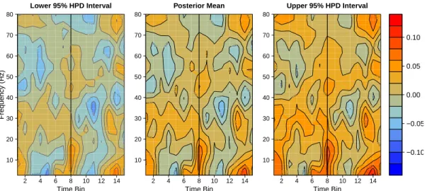
indicates the approximate time at which the rat processed the stimuli,t∗. . . 31 2.5 Pointwise 95% HPD intervals and the posterior mean for µ¯(3)_t ,

which is the average difference in squared coherence between the FC and FS trials. The black vertical lines indicate the event timet∗. . . 36 3.1 Bayesian trend filtering (D = 2) with dynamic horseshoe process

in-novations of minute-by-minute CPU usage data. (a) Observed datayt (points), posterior expectation (cyan) of βt, and 95% pointwise high-est posterior density (HPD) credible intervals (light gray) and 95% si-multaneous credible bands (dark gray) for the posterior predictive dis-tribution of yt. (b) Second difference of observed data ∆2yt (points), posterior expectation of ωt = ∆2βt (cyan), and 95% pointwise HPD intervals (light gray) and simultaneous credible bands (dark gray) for the posterior predictive distribution of ∆2_y

t. (c) Posterior expectation of time-dependent observation standard deviations, σt. (d) Posterior expectation of time-dependent innovation (prior) standard deviations,

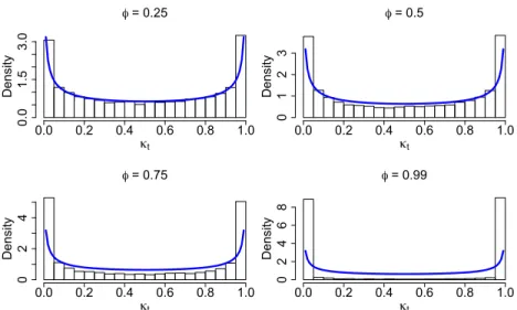
τ λt. . . 42 3.2 Simulation-based estimate of the stationary distribution ofκtfor

various AR(1) coefficients φ. The blue line indicates the density ofκtin the static (φ= 0) horseshoe,[κ]∼Beta(1/2,1/2). . . 48 3.3 Fitted curves for simulated data with T = 128and RSNR = 7.

Each panel includes the simulated observations (x-marks), the posterior expectations of βt(cyan), and the 95% pointwise HPD credible intervals (light gray) and 95% simultaneous credible bands (dark gray) for the posterior predictive distribution of{yt} under BTF-DHS model (3.8) with D = 2. The proposed esti-mator, as well as the uncertainty bands, accurately capture both slowly- and rapidly-changing behavior in the underlying func-tions. . . 56

(12)

3.4 Root mean squared errors for simulated data with T = 128and RSNR = 7. The Bayesian trend filtering (BTF) estimators differ in their innovation distributions, which determines the shrink-age behavior of the second order differences (D = 2): normal-inverse-Gamma (NIG), horseshoe (HS), and dynamic horseshoe (DHS). . . 58 3.5 Root mean squared error for out-of-sample minute-by-minute CPU

us-age data. The Bayesian trend filtering (BTF) estimators differ in their innovation distributions, which determines the shrinkage behavior of the second order differences (D = 2): normal-inverse-Gamma (NIG), horseshoe (HS), and dynamic horseshoe (DHS). . . 60 3.6 True regression functionsβ_j,t∗ (black line) and corresponding

pos-terior expectations (cyan), 95% pointwise HPD credible intervals (light gray) and 95% simultaneous credible bands (dark gray) for

βj,tunder the BTF-DHS model given by (3.9) and (3.10) for a sim-ulated data set. . . 63 3.7 Root mean squared errors for the regression coefficients, β_j,t∗

(left) and the true curves,y_t∗ =x0_tβ∗_t (right) for simulated data. . 64 3.8 Posterior expectations (cyan), 95% pointwise HPD credible

in-tervals (light gray) and 95% simultaneous credible bands (dark gray) for βj,t and σt (bottom right) under the BTF-DHS model given by (3.9) and (3.10) for value-weighted manufacturing in-dustry returns. The solid black line is zero, the dashed green line is the ordinary linear regression estimate, and the solid red line indicates periods for which the 95% simultaneous credible bands do not contain zero. . . 67 3.9 Posterior expectations (cyan), 95% pointwise HPD credible

in-tervals (light gray) and 95% simultaneous credible bands (dark gray) for βj,t and σt (bottom right) under the BTF-DHS model given by (3.9) and (3.10) for value-weighted healthcare industry returns. The solid black line is zero, the dashed green line is the ordinary linear regression estimate, and the solid red line indi-cates periods for which the 95% simultaneous credible bands do not contain zero. . . 68 4.1 Sample paths of t and Yt = µt +µ as a function of τ, where

t is a Gaussian process with the Mat´ern correlation function, ρ = (ρ1,0.1), σ = 0.01, and Yt is generated using the Bimodal-Gaussian FAR(1) kernel,t = 1, . . . , T = 50. The curves are time-ordered by color (from red/orange to blue/violet). Left to right:

t(τ), ρ1 = 2.5;t(τ), ρ1 = 0.5;Yt(τ), ρ1 = 2.5;Yt(τ), ρ1 = 0.5. Note

that we do not observeYtdirectly, but ratheryi,t = Yt(τi,t) +νi,t, where νi,t ∼ N(0, σ2ν) is measurement error with σν = σ/5 =

(13)

4.2 M SF Ee under various designs. Top left: FAR(1), T = 350, sparse-random design with the Linear-ukernel and smooth GP innovations. Top right: FAR(1),T = 50, sparse-random design with the Bimodal-Gaussian kernel and non-smooth GP innova-tions. Bottom left: FAR(1), T = 350, sparse-fixed design with the Bimodal-Gaussian kernel and smooth GP innovations. Bot-tom right: FAR(2), T = 125, sparse-fixed design with Bimodal-Gaussian and Linear−τ kernels and smooth GP innovations. The proposed methods provide superior forecasts and nearly achieve the oracle performance, despite the presence of sparsity. 99 4.3 M SEψ1 under various designs. Top left: FAR(1), T = 350,

sparse-random design with the Linear-ukernel and smooth GP innovations. Top right: FAR(1),T = 50, sparse-random design with the Bimodal-Gaussian kernel and non-smooth GP innova-tions. Bottom left: FAR(1), T = 350, sparse-fixed design with the Bimodal-Gaussian kernel and smooth GP innovations. Bot-tom right: FAR(2), T = 125, sparse-fixed design with Bimodal-Gaussian and Linear−τ kernels and smooth GP innovations. Es-timates ofψ1 are far superior for the proposed methods,

includ-ing the FAR(p) with model averaging. . . 100 4.4 One-step nominal (left) and real (right) yield curve forecasts

during 2016. Top: Time series of five (×) and ten (4) year ob-served maturities with one-step forecasts. Bottom: Observed (points) and forecast (line) curves on 8/2/16, corresponding to the dotted vertical line in the top panels. Posterior means (blue) and 95% pointwise and simultaneous prediction bands (light gray and dark gray, respectively) estimated using 10,000 MCMC simulations after a burn-in of 5,000. . . 104 A.1 Pointwise 95% HPD intervals and the posterior mean for µ¯(1)_t ,

which is the average difference in the PFC log-spectra between the FC and FS trials. The black vertical lines indicatet∗. . . 119 A.2 Pointwise 95% HPD intervals and the posterior mean for µ¯(2)_t ,

which is the average difference in the PFC log-spectra between the FC and FS trials. The black vertical lines indicatet∗. . . 120 A.3 The observed volatility clustering from the yield curve

applica-tion. The black lines are the posterior means of the squared resid-uals from the AR(1) process on theω(_k,tc)in the common trend hid-den Markov model of Section 2.4.1. The red lines are the poste-rior means of the corresponding volatility estimates σ2_k,₍_c₎_,t dis-cussed in Section 2.4.1. . . 121

(14)

B.1 Computation time per 1000 MCMC iterations for the Bayesian trend filtering model with dynamic horseshoe innovations (BTF-DHS). . . 127 C.1 M SF Ee (top) and corresponding M SEψ1 (bottom) under

var-ious designs. Left: FAR(1), T = 50, dense design with the Bimodal-Gaussian kernel and non-smooth GP innovations. Right: FAR(1), T = 350, dense design with the Bimodal-Gaussian kernel and smooth GP innovations. The proposed methods provide superior forecasts and nearly achieve the or-acle performance, despite the presence of sparsity. . . 147 C.2 The Bimodal-Gaussian kernel, ψ(τ, u) ∝ 0.75

π(0.3)(0.4)exp{−(τ − 0.2)2_/₍₀_.₃₎2₋₍_u₋₀_.₃₎2_/₍₀_.₄₎2_}₊ 0.45 π(0.3)(0.4)exp{−(τ−0.7) 2_/₍₀_.₃₎2₋ (u−0.8)2_/₍₀_.₄₎2_}_{, normalized so that}R R ψ2 `(τ, u)dτ du= 0.8. . . 148 C.3 Traceplot for one-step forecasts for nominal yield curves at

se-lected maturities during 2016. . . 150 C.4 Traceplot for one-step forecasts for real yield curves at selected

maturities during 2016. . . 151 E1 Standardized squared errors and relative absolute errors for

smooth (top) and non-smooth (bottom) integrands. The errors are small in magnitude, particularly in the smooth case, and de-cay quickly forM >20. . . 153

(15)

CHAPTER 1 INTRODUCTION

We present Bayesian methodology for modeling functional and time series data. The methods are broadly applicable for (dependent) functional and time series data, but we focus in particular on the following challenging cases for which existing methods are inadequate:

1. Functional data with additional complex dependence, such as time depen-dence, contemporaneous dependepen-dence, stochastic volatility, covariates, and change points (Chapter 2);

2. Functional data, time series data, or regression functions with local fea-tures, such as jumps or rapidly-changing smoothness (Chapter 3); and

3. Forecasting and inference of functional time series data with sparsely or irregularly sampled curves and for curves sampled with non-negligible measurement error (Chapter 4).

A unifying characteristic of the proposed methods is the employment of the dynamic linear model (DLM) framework in new contexts to construct inter-pretable models and computationally efficient MCMC sampling algorithms. In particular, we develop highly efficient Gibbs sampling algorithms that build upon existing DLM sampling components for large blocks of parameters (e.g., Rue, 2001; Durbin and Koopman, 2002). The novel applications of DLMs in-clude functional dynamic factor models, Bayesian trend filtering models, dy-namic shrinkage processes (see Chapter 3), and functional autoregressive mod-els. Importantly, the Bayesian framework permits joint estimation of the model

(16)

parameters and provides exact inference (up to MCMC error) on specific pa-rameters.

The proposed methodology is motivated by important applications includ-ing multi-economy interest rate modelinclud-ing, nominal and real yield curve fore-casting, dynamic extensions of the Fama-French asset pricing model, irregular curve-fitting of CPU usage data, and local field potential brain signals in rats. The methods are evaluated through extensive simulations, and compared to state-of-the-art alternative estimators, with favorable results.

In Chapter 2, we present a Bayesian model for multivariate, dependent tional data, in which we extend DLMs for multivariate time series to the func-tional data setting. We also develop Bayesian spline theory in a more general constrained optimization framework. The proposed methods identify a time-invariant functional basis for the functional observations, which is smooth and interpretable. We apply the methodology to study the interactions of multi-economy yield curves during the recent global recession, and analyze local field potential brain signals in rats, for which we develop a multivariate functional time series approach for multivariate time-frequency analysis.

In Chapter 3, we propose a novel class of dynamic shrinkage processes for Bayesian time series and regression analysis. We extend a broad class of popular global-local shrinkage priors, such as the horseshoe prior, to the dynamic setting by allowing the local scale parameters to depend on the history of the shrinkage process. We prove that the resulting processes inherit desirable shrinkage be-havior from the non-dynamic analogs, but provide additional locally adaptive shrinkage properties. The proposed dynamic shrinkage processes are widely applicable, particularly within the family of dynamic linear models. By

(17)

express-ing dynamic shrinkage processes on the log-scale, we adapt successful tech-niques from stochastic volatility modeling, and propose a P ´olya-Gamma scale mixture representation to produce a highly efficient Gibbs sampling algorithm. We use the proposed processes to produce superior Bayesian trend filtering es-timates and posterior credible intervals for irregular curve-fitting of minute-by-minute Twitter CPU usage data, and develop an adaptive time-varying param-eter regression model to assess the efficacy of the Fama-French five-factor asset pricing model with momentum added as a sixth factor.

In Chapter 4, we develop a hierarchical Gaussian process model for forecast-ing and inference of functional time series data. Unlike existforecast-ing methods, our approach is especially suited for sparsely or irregularly sampled curves and for curves sampled with non-negligible measurement error. The latent pro-cess is dynamically modeled as a functional autoregression (FAR) with Gaus-sian process innovations, with extensions for FAR(p) models with model aver-aging over the lag p. We propose a fully nonparametric dynamic functional factor model for the dynamic innovation process, with broader applicability and improved computational efficiency over standard Gaussian process mod-els. We prove finite-sample forecasting and interpolation optimality properties of the proposed model, which remain valid with the Gaussian assumption re-laxed. Extensive simulations demonstrate substantial improvements in fore-casting performance and recovery of the autoregressive surface over competing methods, especially under sparse designs. We apply the proposed methods to forecast nominal and real yield curves using daily U.S. data. Real yields are ob-served more sparsely than nominal yields, yet the proposed methods are highly competitive in both settings.

(18)

CHAPTER 2

A BAYESIAN MULTIVARIATE FUNCTIONAL DYNAMIC LINEAR MODEL

Portions of this chapter were published in Kowal et al. (2016).

2.1

Introduction

We consider a multivariate time series of functional data. Functional data anal-ysis (FDA) methods are widely applicable, including diverse fields such as eco-nomics and finance (e.g., Hays et al., 2012); brain imaging (e.g., Staicu et al., 2012); chemometric analysis, speech recognition, and electricity consumption (Ferraty and Vieu, 2006); and growth curves and environmental monitoring (Ramsay and Silverman, 2005). Methodology for independent and identically distributed (iid) functional data has been well-developed, but in the case of de-pendentfunctional data, the iid methods are not appropriate. Such dependence is common, and can arise via multiple responses, temporal and spatial effects, repeated measurements, missing covariates, or simply because of some natural grouping in the data (e.g., Horv´ath and Kokoszka, 2012). Here, we consider two distinct sources of dependence: time dependence for time-ordered functional observations and contemporaneous dependence for multivariate functional ob-servations.

Suppose we observe multiple functions Y_t(c)(τ), c = 1, . . . , C, at time points

t= 1, . . . , T. Such observations have three dominant features:

(19)

(b) For eachcandτ,Y_t(c)(τ)is atime seriesfort= 1, . . . , T; and

(c) For each t and τ, Y_t(c)(τ) is a multivariate observation with outcomes c = 1, . . . , C.

We assume thatT ⊆_Rd_{is compact, and focus on the case}_d _{= 1}_{in which}_τ _{is a} scalar. However, our approach may be adapted to the more general setting.

We consider two diverse applications of multivariate functional time series (MFTS).

Multi-Economy Yield Curves: LetY_t(c)(τ)denotemulti-economy yield curves ob-served on weekst = 1, . . . , T for economiesc= 1, . . . , C, which refer to the Fed-eral Reserve, the Bank of England, the European Central Bank, and the Bank of Canada. For a given currency and level of risk of a debt, the yield curve de-scribes the interest rate as a function of the length of the borrowing period, or time to maturity, τ. Yield curves are important in a variety of economic and financial applications, such as evaluating economic and monetary conditions, pricing fixed-income securities, generating forward curves, computing infla-tion premiums, and monitoring business cycles (Bolder et al., 2004). We are particularly interested in the relationships among yield curves for the aforemen-tioned globally-influential economies, and in how these relationships vary over time. However, existing FDA methods are inadequate to model the dynamic de-pendences among and between the yield curves for different economies, such as contemporaneous dependence, volatility clustering, covariates, and change points. Our approach resolves these inadequacies, and provides useful insights into the interactions among multi-economy yield curves (see Section 2.4.1).

(20)

peri-odic behavior of the process is often the primary interest. Time-frequency anal-ysisis used when this periodic behavior varies over time, which requires con-sideration of both the time and frequency domains (e.g., Shumway and Stof-fer, 2000). Typical methods segment the multivariate time series into (overlap-ping) time bins within which the periodic behavior is approximately stationary; within each bin, standard frequency domain or spectral analysis is performed, which uses the multivariate discrete Fourier transform of the time series to iden-tify dominant frequencies. Interestingly, although the raw signal in this set-ting is a multivariate time series, time-frequency analysis produces a MFTS: the multivariate discrete Fourier transform is afunctionof frequencyτ fortime

bins t = 1, . . . , T, where c = 1, . . . , C index themultivariatecomponents of the spectrum. We analyze local field potential (LFP) data collected on rats, which measures the neural activity of local brain regions over time (Ljubojevic et al., 2013). Our interest is in the time-dependent periodic behavior of these local brain regions under different stimuli, and in particular the synchronization be-tween brain regions. Our novel MFTS approach to time-frequency analysis pro-vides the necessary multivariate structure and inference—which is unavailable in standard time-frequency analysis—to precisely characterize brain behavior under certain stimuli (see Section 2.4.2).

To model MFTS, we extend the hierarchical dynamic linear model (DLM) framework of Gamerman and Migon (1993) and West and Harrison (1997) for multivariate time series to the functional data setting. For smooth, flexible, and optimal function estimates, we extend Bayesian spline theory to a more general constrained optimization framework, which we apply for parameter identifi-ability. Our constraints are explicit in the posterior distribution via appropri-ate conditioning of the standard Bayesian spline posterior distribution, and the

(21)

corresponding posterior mean is the solution to an appropriate optimization problem. We implement an efficient Gibbs sampler to obtain samples from the joint posterior distribution, which provides exact (up to MCMC error) inference for any parameters of interest. The proposed hierarchical BayesianMultivariate Functional Dynamic Linear Model has greater applicability and utility than re-lated methods. It provides flexible modeling of complex dependence structures among the functional observations, such as time dependence, contemporane-ous dependence, stochastic volatility, covariates, and change points, and can incorporate application-specific prior information.

The paper proceeds as follows. In Section 2.2, we present our model in its most general form. We develop our (factor loading) curve estimation technique in Section 2.3. In Section 2.4, we apply our model to the two applications dis-cussed above and interpret the results. We also provide the details of our Gibbs sampling algorithm, present MCMC diagnostics for our applications, and in-clude additional figures in Appendix A.

2.2

A Multivariate Functional Dynamic Linear Model

Suppose we observe functions Y_t(c): T → _Rat times t = 1, . . . , T for outcomes

c = 1, . . . , C, where T ⊆ _Ris compact. We refer to the following model as the

(22)

               Yt(τ) =F(τ)βt+t(τ), t(τ) E_t indep ∼ N(0,Et), β_t =Xtθt+νt, νt V_t indep ∼ N(0,Vt), θt =Gtθt−1+ωt, ωt W_t indep ∼ N(0,Wt), (2.1) where Yt(τ) = h Y_t(1)(τ), Y_t(2)(τ), . . . , Y_t(C)(τ) i0

is the C-dimensional vector of multivariate functional observations at time t evaluated at τ ∈ T; F(τ)is the

C×KCblock matrix with1×Kdiagonal blockshf₁(c)(τ), f₂(c)(τ), . . . , f_K(c)(τ)ifor

c = 1, . . . , C offactor loading curves evaluated atτ ∈ T, with K the number of factors per outcome, and zeros elsewhere;β_t = hβ₁(1)_,t, . . . , β_K,t(1), β₁(2)_,t, . . . , β_K,t(C)i

0 is theKC-dimensional vector offactorsthat serve as the time-dependent weights on the factor loading curves; Xt is the known KC ×p matrix of covariates at timet, wherepis the total number of covariates;θtis thep-dimensional vector of regression coefficients associated with Xt; Gt is the p×p evolution matrix of the regression coefficientsθt at timet; andt(τ), νt,andωtare mutually in-dependent error vectors with variance matrices Et, Vt, and Wt, respectively. We assume conditional independence of [t(τ)|Et] over both t = 1, . . . , T and

τ ∈ T; however, the latter assumption of independence overτ may be relaxed. We can immediately obtain a useful submodel of (2.1) by excluding covariates,

Xt = ICK×CK, and removing a level of the hierarchy, Vt = 0CK×CK, so that settingGt = G models βt (= θt, almost surely) with a vector autoregression (VAR).

To understand (2.1), first note that the observation level of the model com-bines thefunctionalcomponentF(τ)with themultivariate time seriescomponent β_t. In scalar notation, we can write the observation level as

Y_t(c)(τ) =

K X k=1

(23)

in which (_tc)(τ) are the elements of the vector t(τ). In our construction, we can always write the observation level of (2.1) as (2.2); simplifications for the other levels will depend on the choice of submodel. For model identifiability, we require orthonormality of the factor loading curves:

Z τ∈T

f_k(c)(τ)f_j(c)(τ)dτ =1(k =j) (2.3) fork, j = 1, . . . , Kand all outcomesc= 1, . . . , C, where1(·)is the indicator func-tion. In addition, to ensure a unique and interpretable ordering of the factors

β₁(c_,t), . . . , β_K,t(c) for each outcomec = 1, . . . , C, we order the factor loading curves

f₁(c), . . . , f_K(c)by decreasing smoothness. We discuss our implementation of these constraints in Sections 2.3.2 and 2.3.3.

There are three primary interpretations of the model, which provide insight into useful extensions and submodels.

First, we can view (2.2) as a basis expansion of the functional observations

Y_t(c), with a (multivariate) time series model for the basis coefficientsβ_k,t(c) to ac-count for the additional dependence structures, such as common trends (see Section 2.4.1), stochastic volatility (see Section 2.4.1), and covariates. Since the identifiability constraint in (2.3) expresses orthonormality with respect to theL2

inner product, we can interpretnf₁(c), . . . , f_K(c)oas an orthonormal basis for the functional observationsY_t(c). In contrast to common basis expansion procedures that assume the basis functions are known and only the coefficients need to be estimated (e.g., Bowsher and Meeks, 2008), we allow our basis functionsf_k(c) to be estimated from the data. As a result, the f_k(c) will be more closely tailored to the data, which reduces the number of functions K needed to adequately fit the data. Conditional on the f_k(c), we can specify the β_t- and θt-levels of (2.1) to appropriately model the remaining dependence among theY_t(c). Using

(24)

this interpretation, we also note that (2.1) may be described as a multivariate dynamic (concurrent) functional linear model, and therefore extends a highly useful model in FDA (Cardot et al., 1999).

Similarly, we can interpret (2.1) as a dynamic factor analysis, which is a com-mon approach in yield curve modeling (e.g., Hays et al., 2012; Jungbacker et al., 2013). Under this interpretation, theβ_k,t(c)are dynamicfactorsand thef_k(c)are fac-tor loading curves(FLCs); we will use this terminology for the remainder of the paper. Compared to a standard factor analysis, (2.1) has two major modifica-tions: the factorsβ_k,t(c) are dynamic and therefore have an accompanying (multi-variate) time series model, and thef_k(c)are functions rather than vectors.

Naturally, (2.1) has strong connections to a hierarchical DLM. Stan-dard hierarchical DLM algorithms for sampling β_t and θt assume that {F,Gt,Xt,Et,Vt,Wt}is known (e.g., Durbin and Koopman, 2002; Petris et al., 2009). Within our Gibbs sampler, we may condition on this set of parame-ters, and then use existing DLM algorithms to efficiently sample β_t and θt with minimal implementation effort. Unconditionally, F is unknown, but we impose the necessary identifiability constraints; see Section 2.3 for more de-tails. Gt may be known or unknown depending on the application, but in general it supplies the time series structure of the model (along with the time-dependent error variances): in Section 2.4.1, Gt = G is unknown to allow for data-driven dependence among the multi-economy yield curves, and in Section 2.4.2,Gt =ICK×CKis chosen to provide parsimonious time-domain smoothing. We assume that Xt is known, and may consist of covariates relevant to each outcome or can be chosen to provide additional shrinkage ofβ_tthroughθt. Al-though Gamerman and Migon (1993) suggest thatdim(θt) < dim(βt)for strict

(25)

dimension reduction in the hierarchy, we relax this assumption to allow for co-variate information. Finally, we treat the error variance matrices as unknown, but typically there are simplifications available depending on the application and model choice. We discuss some examples in Section 2.4.

We must also specify a choice for K. In the yield curve application, two natural choices are K = 3and K = 4for comparison with the common para-metric yield curve models: the Nelson-Siegel model (Nelson and Siegel, 1987) and the Svensson model (Svensson, 1994), both of which can be expressed as submodels of (2.1); see Diebold and Li (2006) and Laurini and Hotta (2010). More formally, we can treat K as a parameter and estimate it using reversible jump MCMC methods (Green, 1995), or selectK using marginal likelihood. In particular, since we employ a Gibbs sampler, the marginal likelihood estima-tion procedure of Chib (1995) is convenient for many submodels of (2.1). For more complex models, DIC provides a less computationally intensive approach than either reversible jump MCMC or marginal likelihood, and is very simple to compute. In Appendix A, we discuss a fast procedure based on the singu-lar value decomposition from our initialization algorithm which can be used to estimate a range of reasonable values forK.

2.3

Estimating the Factor Loading Curves

We would like to model the FLCsf_k(c)in a smooth, flexible, and computationally appealing manner. Clearly, the latter two attributes are important for broader applicability and larger data sets—including largerT, largerC, and largerm(_tc), where m(_tc) denotes the number of observation points for outcome cat time t.

(26)

The smoothness requirement is fundamental as well: as documented in Jung-backer et al. (2013), smoothness constraints can improve forecasting, despite the small biases imposed by such constraints. Smooth curves also tend to be more interpretable, since gradual trends are usually easier to explain than sharp changes or discontinuities.

However, there are some additional complications. First, we must incorpo-rate the identifiability constraints, preferably without severely detracting from the smoothness and goodness-of-fit of the FLCs. We also haveK curves to es-timate for each outcome—or perhaps K curves common to all outcomes (see Section 2.3.4)—similar to the varying-coefficients model of Hastie and Tibshi-rani (1993), conditional on the factorsβ_k,t(c). Finally, the observation points for the functions Y_t(c) are likely different for each outcome c, and may also vary with timet.

2.3.1

Splines

A common approach in nonparametric and semiparametric regression is to ex-press each unknown functionf_k(c) as a linear combination of known basis func-tions, and then estimate the associated coefficients by maximizing a (penalized) likelihood (e.g., Wahba, 1990; Eubank, 1999; Ruppert et al., 2003). We use B-spline basis functions for their numerical properties and easy implementation, but our methods can accommodate other bases as well. For now, we ignore dependence oncfor notational convenience; this also corresponds to either the univariate case(C = 1)orC >1withEtdiagonal and the FLCs assumed to be

(27)

alterna-tive). Following Wand and Ormerod (2008), we use cubic splines and the knot sequencea = κ1 = . . . = κ4 < κ5 < . . . < κM+4 < κM+5 = . . . = κM+8 = b,

withφ_B = (φ1, . . . , φM+4)the associated cubic B-spline basis,M the number of

interior knots, and T = [a, b]. While we could allow each fk to have its own B-spline basis and accompanying sequence of knots, there is no obvious reason to do so. In our applications, we useM = 20interior knots. For knot placement, we prefer a quantile-based approach such as the default method described in Ruppert et al. (2003), which is responsive to the location of observation points in the data yet is computationally inexpensive; however, equally-spaced knots may be preferable in some applications.

Explicitly, we writefk(τ) = φ0B(τ)dk, wheredk is the(M + 4)-dimensional vector of unknown coefficients. Therefore, the function estimation problem is reduced to a vector estimation problem. In classical nonparametric regression, dkis estimated by maximizing a penalized likelihood, or equivalently solving

min

dk

−2 log[Y|dk] +λkP(dk) (2.4)

where [Y|dk] is a likelihood, P is a convex penalty function, and λk ≥ 0. We express (2.4) as a log-likelihood multiplied by−2so that for a Gaussian likeli-hood, (2.4) is simply a penalized least squares objective. For greater generality, we leave the likelihood unspecified, but later consider the likelihood of model (2.2). To penalize roughness, a standard choice forP is theL2-norm of the sec-ond derivative offk, which can be written in terms ofdk:

P(dk) = Z τ∈T h ¨ fk(τ) i2 dτ =d0_kΩφdk (2.5)

where f¨k denotes the second derivative of fk and Ωφ = R

T φ¨B(τ) ¨φB 0

(τ) dτ, which is easily computable for B-splines. With this choice of penalty, (2.4) bal-ances goodness-of-fit with smoothness, where the trade-off is determined by

(28)

λk.

SinceP is a quadratic indk, for fixedλk, (2.4) is straightforward to solve for many likelihoods, in particular a Gaussian likelihood. Letting d¯k be this solu-tion, we can estimatefk(τ)for any τ ∈ T with fˆk(τ) = φ0B(τ)d¯k. For a general knot sequence, the resulting estimatorfˆkis an O’Sullivan spline, orO-spline, in-troduced by O’Sullivan (1986) and explored in Wand and Ormerod (2008). In the special case of univariate nonparametric regression in which there is a knot at every observation point, fˆk is a natural cubic smoothing spline (e.g., Green and Silverman, 1993). Alternatively, if we choose a sparser sequence of knots and setλk = 0, fˆk is a regression spline (e.g., Ramsay and Silverman, 2005). O-splines are numerically stable, possess natural boundary properties, and can be computed efficiently (cf. Wand and Ormerod, 2008).

2.3.2

Bayesian Splines

Splines also have a convenient Bayesian interpretation (e.g., Wahba, 1978, 1983, 1990; Gu, 1992; Van der Linde, 1995; Berry et al., 2002). Returning to (2.4), we no-tably have a likelihood term and a penalty term, where the penalty is a function of only the vector of coefficients dk and known quantities. Therefore, condi-tional onλk, the termλkP(dk)provides prior information aboutdk, for example that fk = φ0Bdk is smooth. Under this general interpretation, (2.4) combines the prior information with the likelihood to obtain an estimate ofdk. A natural Bayesian approach is therefore to construct a prior fordk based on the penalty P, in particular so that the posterior mode ofdk is the solution to (2.4). For the most common settings in which the likelihood is Gaussian and the penalty P

(29)

is (2.5), the posterior distribution ofdkwill be Gaussian, so the posterior mean will also solve (2.4).

To construct a prior from P, it is computationally and conceptually con-venient to reparameterize dk so that the penalty matrix Ωφ is diagonal. Un-der a Gaussian prior, this corresponds to prior independence of the compo-nents ofdk. The reparameterization will also affect the basisφB, but otherwise will leave the likelihood in (2.4) unchanged. Following Wand and Ormerod (2008), let Ωφ = UΩDΩU0Ω be the singular value decomposition of Ωφ, where

U0_ΩUΩ =I(M+4)×(M+4) andDΩis a diagonal matrix withM + 2positive

compo-nents. Denote the diagonal matrix of these positive entries byDΩ,P and letUΩ,P be the corresponding(M + 4)×(M + 2)submatrix ofUΩ. Using the

reparam-eterized basisφ0(τ) = h1, τ,φ0_B(τ)UΩ,PD −1/2 Ω,P

i

and penaltyd0_kΩDdk with ΩD = diag(0,0, λk, . . . , λk), the new solution dˆk to (2.4) satisfies fˆk(τ) = φB(τ)d¯k = φ0(τ)dˆk; see Wand and Ormerod (2008) for more details. It is therefore natural to use the prior dk ∼ N(0,Dk), where Dk = diag 108,108, λ−k1, . . . , λ

−1

k

and

λk > 0, which satisfies D−k1 ≈ ΩD. Notably, this prior is proper, yet is diffuse over the space of constant and linear functions—which are unpenalized by P. This reparameterization is a common approach for fitting splines using mixed effects model software (e.g., Ruppert et al., 2003).

Since we assume conditional independence between levels of (2.1), our con-ditional likelihood for the FLCs is simply that of model (2.2), but we ignore dependence oncfor now:

Yt(τ) = K X k=1 βk,tfk(τ) +t(τ) = K X k=1 βk,tφ0(τ)dk+t(τ) (2.6) wheret(τ) iid

∼ N(0, σ2₎_{for simplicity; the results are similar for more}

(30)

the functional dataYtgiven the FLCsfk(ordk), also conditional onβk,tandσ2. Under the likelihood of model (2.6) and the reparameterized (approxi-mate) penalty d0_kD−_k1dk, the solution to (2.4) conditional on dj, j 6= k is given by dˆk = Bkbk where B−k1 = D −1 k +σ −2PT t=1β 2 k,t P τ∈Ttφ(τ)φ 0 (τ), bk = σ−2PT t=1βk,t P τ∈Tt h Yt(τ)− P j6=kβj,tfj(τ) i

φ(τ), and Tt ⊆ T denotes the dis-crete set of|Tt| =mtobservation points forYtat timet. Note that ifTt = T1 for

t = 2, . . . , T, thenBk andbkmay be rewritten more conveniently in vector no-tation. Most importantly for our purposes, under the same likelihood induced by (2.6) and the prior dk ∼ N(0,Dk), the posterior distribution of dk is multi-variate Gaussian with meandˆkand varianceBk. For convenient computations, Wand and Ormerod (2008) provide an exact construction ofΩφand suggest effi-cient algorithms fordˆkbased on the Cholesky decomposition; we provide more details in Appendix A.

To identify the ordering of the factors and FLCs in (2.2), we constrain the smoothing parametersλ1 > λ2 > · · · > λK >0. While other model constraints are available, this ordering constraint is particularly appealing: it sorts the FLCs

fk by decreasing smoothness, as characterized by the penalty functionP, and leads to a convenient prior distribution on the smoothing parameters λk. In the Bayesian setting, the smoothing parameters are equivalently the prior preci-sions of the penalized (nonlinear) components ofdk. Lettingdk,jdenote thejth component ofdk, the prior on the FLC basis coefficients isdk,j

iid

∼ N(0, λ−_k1)for

j = 3, . . . , M + 4. This is similar to the hierarchical setting of Gelman (2006), in which there areM+ 2groups for eachλk, k = 1, . . . , K. SinceM+ 2is typically large, we follow the Gelman (2006) recommendation to place uniform priors on the group standard deviations λ−_k1/2, k = 1, . . . , K. Incorporating the ordering

(31)

constraint, the conditional priors are λ−_k1/2 ∼ Uniform(`k, uk), where `1 = 0, `k = λ −1/2 k−1 for k = 2, . . . , K, uk = λ −1/2 k+1 for k = 1, . . . , K −1, and uK = 104. The upper bound onλ−_K1/2, and therefore allλ−_k1/2, is chosen to equal the diffuse prior standard deviation of dk,1 and dk,2. The full conditional distributions of

the smoothing parametersλk are Gamma 1 2(M+ 1), 1 2 PM+4 j=3 d2k,j truncated to

(u−_k2, `−_k2)fork = 1, . . . , K, where we define`−₁2 =∞. Notably, we avoid the dif-fuse Gamma prior onλk, which can be undesirably informative and is strongly discouraged by Gelman (2006). More generally, our approach provides a natu-ral and data-driven method for estimating the smoothing parameters, yet does not inhibit inference. Details on the sampling ofλk are provided in Appendix A.

2.3.3

Constrained Bayesian Splines

We extend the Bayesian spline approach to accommodate the necessary iden-tifiability constraints for the MFDLM. For each k = 1, . . . , K, we impose the orthonormality constraintsR

T fk(τ)fj(τ) = 1(k = j)forj = 1, . . . , K. The unit-norm constraint preserves identifiability with respect to scaling, i.e., relative to the factorsβk,t(up to changes in sign). The orthogonality constraints distinguish between pairs of FLCs, and in our approach identify the FLCs with distinct pos-terior distributions.

While other identifiability constraints are available for thefk, orthonormality is appealing for a number of reasons. As discussed in Section 2.2, the orthonor-mality constraints suggest that we can interpret{f1, . . . , fK}as an orthonormal basis for the functional observationsYt. As such, the orthogonality constraints

(32)

help eliminate any information overlap between FLCs, which keeps the total number of necessary FLCs to a minimum. Furthermore, the unit norm con-straint allows for easier comparisons among the fk. Of course, the fk will be weighted by the factorsβk,t, so they can still have varying effects on the condi-tional mean ofYtin (2.2). Finally, we can write the constraints conveniently in terms of the vectorsdkanddj:

Z τ∈T fk(τ)fj(τ)dτ = Z τ∈T φ0(τ)dkφ0(τ)dj dτ =d0kJφdj =1(k =j) (2.7) forj = 1, . . . , K, whereJφ = R τ∈T φ(τ)φ 0

(τ)dτ is easily computed for B-splines, and only needs to be computed once, prior to any MCMC sampling.

The addition of an orthogonality constraint to a (penalized) least squares problem has an intuitive regression-based interpretation, which we present in the following theorem:

Theorem 2.1. Consider the penalized least squares objectiveσ−2Pn

i=1(yi−X

0 id)2 +

λd0Ωd, whereyi ∈ R, dis an unknown (M + 4)-dimensional vector,Xi is a known

(M+ 4)-dimensional vector,Ωis a known(M+ 4)×(M+ 4)positive-definite matrix, and σ2_{, λ >} ₀ _{are known scalars. The solution is} _d_ˆ ₌ _Bb_{, where} _B−1 ₌ _λ_Ω ₊

σ−2Pn

i=1XiX0i andb =σ−2 Pn

i=1Xiyi. Now consider the same objective, but subject

to theJ linear constraintsd0L =0forLa known(M + 4)×J matrix of rankJ. The solution isd˜=B˜b, whereb˜is the vector of residuals from the generalized least squares regressionb =LΛ+δ withE(δ) = 0andVar(δ) = B.

Proof. The optimality ofdˆis a well-known result. For the constrained case, the Lagrangian isL(d,Λ) = σ−2Pn i=1(yi −X 0 id)2 +λd 0 Ωd+d0LΛ, where Λis the

J-dimensional vector of Lagrange multipliers associated with theJ linear con-straints. It is straightforward to minimizeL(d,Λ)with respect to dand obtain

(33)

the solutiond˜=B˜b=B(b−LΛ). Similarly, solving∇L(d˜,Λ) = 0forΛimplies thatΛ = (L0BL)−1_L0_Bb

, which is the solution to the generalized least squares regression ofbonLwith error varianceB.

The result is interpretable: to incorporate linear constraints into a penalized least squares regression, we find˜bnearest tobunder the inner product induced byB among vectors in the space orthogonal to Col(L). In our setting, extend-ing (2.4) under a Gaussian likelihood to accommodate the (linear) orthogonality constraintsd0_kJφdj = 0 for j 6= k may be described via a regression of the un-constrained solution on the constraints. However, the unit norm constraint is nonlinear. This constraint affects the scaling but not the shape offk. Therefore, a reasonable approach is to construct a posterior distribution fordkthat respects the (linear) orthogonality constraints only, and then normalize the samples from this posterior to preserve identifiability. We provide more details in Appendix A.

To extend the unconstrained Bayesian splines of Section 2.3.2 to incor-porate the orthogonality constraints, we write the constraints d0_kJφdj =

0 for j 6= k as the linear constraints in Theorem 2.1 with L[−k] =

(Jφd1, . . . ,Jφdk−1,Jφdk+1, . . . ,JφdK) and J = K − 1. Using the full condi-tional posterior distribution dk ∼ N(Bkbk,Bk) from Section 2.3.2, we can ad-ditionally condition on the linear constraints d0_kL[−k] = 0, and obtain the

con-strained full conditional distribution dk ∼ N(B˜kbk,B˜k), where B˜k = Bk −

BkL[−k](L0_[−k]BkL[−k])

−1_L0

[−k]Bk. Conditioning on the orthogonality constraints

is particularly interpretable in the Bayesian setting, and is convenient for pos-terior sampling; see Appendix A for more details. By comparison, Theorem 2.1 implies that the solution to (2.4) under the likelihood of model (2.6), the

(34)

penaltyd0_kD−_k1dk, and subject to the linear constraints d0kL[−k] = 0 is given by

˜

dk = Bk˜bk, where˜bk = bk−L[−k]Λ[−k]and Λ[−k] = (L_[0−k]BkL[−k])

−1_L0

[−k]Bkbk.

Notably, B˜kbk = Bk˜bk = d˜k, which is a useful result: by simply conditioning on the linear orthogonality constraints in the full conditional Gaussian distribu-tion fordk, the posterior mean of the resulting Gaussian distribution solves the constrained regression problem of Theorem 2.1. In this sense, the identifiability constraints onfk are enforced optimally.

2.3.4

Common Factor Loading Curves for Multivariate

Model-ing

Reintroducing dependence on cfor the FLCs f_k(c), suppose thatC > 1, so that our functional time series Y_t(c) is truly multivariate. If we wish to estimate a priori independent FLCs for each outcome c (with Et diagonal), then we can sample from the relevant posterior distributions independently forc= 1, . . . , C

using the methods of Section 2.3.3. The more interesting case is thecommon fac-tor loading curves modelgiven byf_k(c) =fk, so that all outcomes share a common set of FLCs. In the basis interpretation of the MFDLM, this corresponds to the assumption that the functional observations for all outcomesY_t(c),c= 1, . . . , C,

t= 1, . . . , T share a common basis. We find this approach to be useful and intu-itive, since it pools information across outcomes and suggests a more parsimo-nious model. Equally important, the common FLCs approach allows for direct comparison between factorsβ_k,t(c)andβ_k,t(c0)for outcomescandc0, since these fac-tors serve as weights on thesameFLC (or basis function)fk. We use this model in both applications in Section 2.4.

(35)

The common FLCs model implies f_k(c)(τ) = φ0₍_c₎(τ)d(_kc) = fk(τ). However, since the FLCs for each outcome are identical, it is reasonable to assume that they have the same vector of basis functionsφ, sof_k(c) =fkis equivalent tod

(c) k = dk. Moreover, by writing f (c) k (τ) = φ 0

(τ)dk, we can use all of the observation points across all outcomesc= 1, . . . , Cand timest= 1, . . . , T, yet the parameter of interest,dk, will only be(M + 4)-dimensional.

Modifying our previous approach, we use the likelihood of model (2.2) with the simple error distribution (_tc)(τ) iid∼ N(0, σ2

(c)). The implied full

conditional posterior distribution for dk is again N(B˜kbk,B˜k), but now with B−_k1 = D−_k1 + PC c=1σ −2 (c) P t∈T(c)(β (c) k,t)2 P τ∈T_t(c)φ(τ)φ 0 (τ) and bk = PC c=1σ −2 (c) P t∈T(c)β (c) k,t P τ∈T_t(c) h Y_t(c)(τ)−P j6=kβ (c) j,tfj(τ) i

φ(τ). For full generality, we allow the (discrete) set of timesT(c)_{to vary for each outcome}_c_{and the}

(dis-crete) set of observation points T_t(c) to vary with both time t and outcome c, with |T_t(c)| = m(_tc). Note that we reuse the same notation from Section 2.3.3 to emphasize the similarity of the multivariate results to the univariate (ora priori

independent FLC) results. The common notation also allows for a more concise description of the sampling algorithm, which we present in Appendix A.

2.4

Data Analysis and Results

2.4.1

Multi-Economy Yield Curves

We jointly analyze weeklyyield curves provided by the Federal Reserve (Fed), the Bank of England (BOE), the European Central Bank (ECB), and the Bank of Canada (BOC; Bolder et al. 2004) from late 2004 to early 2014 (T = 490andC =

(36)

4). These data are publicly available and published on the respective central bank websites—and as such, we treat them as reliable estimates of the yield curves. For each outcome, the yield curves are estimated differently: the Fed uses quasi-cubic splines, the BOE uses cubic splines with variable smoothing parameters (Waggoner, 1997), the ECB uses Svensson curves, and the BOC uses exponential splines (Li et al., 2001). Therefore, the functional observations have already been smoothed, although by different procedures. The available set of maturitiesT_t(c)is not the same across economiesc, and occasionally varies with time t. The most frequent values ofm(_tc), t = 1, . . . , T, are 11 (Fed), 100 (BOE), 354 (ECB), and 120 (BOC), with maturitiesτ ranging from 1-3 months up to 300-360 months. To facilitate a simpler analysis, we letY_t(c)(τ)be the week-to-week

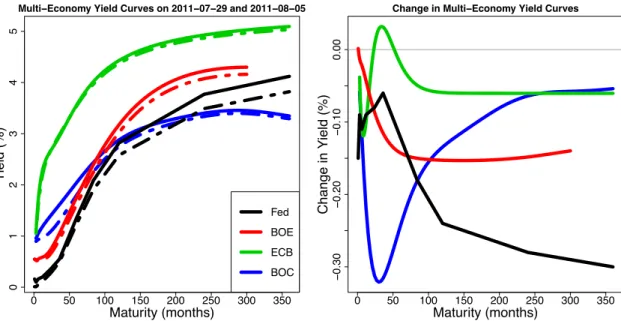
changein thecth central bank yield curve on weektfor maturityτ. Differencing the yield curves conveniently addresses the nonstationarity in the weekly data, and, because the yield curves are pre-smoothed, does not introduce any notable difficulties with time-varying observation points. We show an example of the multi-economy yield curves observed at adjacent times on July 29, 2011 and August 5, 2011, as well as the corresponding one-week change in Figure 2.1.

The literature on yield curve modeling is extensive. Yield curve mod-els commonly adopt the Nmod-elson-Siegel parameterization (Nmod-elson and Siegel, 1987), often within a state space framework (e.g., Diebold and Li, 2006; Diebold et al., 2006, 2008; Koopman et al., 2010). Many Bayesian models also use the Nelson-Siegel or Svensson parameterizations (e.g., Laurini and Hotta, 2010; Cruz-Marcelo et al., 2011). However, the Nelson-Siegel parameterization does not extend to other applications, and often requires solving computationally intensive nonlinear optimization problems. Alternatively, Chib and Ergashev (2009) develop an arbitrage-free affine term structure model, which is similarly

(37)

0 50 100 150 200 250 300 350 0 1 2 3 4 5

Multi−Economy Yield Curves on 2011−07−29 and 2011−08−05

Maturity (months) Y ield (%) Fed BOE ECB BOC 0 50 100 150 200 250 300 350 − 0.30 − 0.20 − 0.10 0.00

Change in Multi−Economy Yield Curves

Maturity (months)

Change in Y

ield (%)

Figure 2.1: Multi-economy yield curves from July 29, 2011 (solid) and August 5, 2011 (dashed), together with the corresponding one-week change curves.

cast in a Bayesian state space framework. More similar to our approach are the Functional Dynamic Factor Model (FDFM) of Hays et al. (2012) and the Smooth Dynamic Factor Model (SDFM) of Jungbacker et al. (2013), both of which fea-ture nonparametric functional components within a state space framework. The FDFM cleverly uses an EM algorithm to jointly estimate the functional and time series components of the model. However, the EM algorithm makes more so-phisticated (multivariate) time series models more challenging to implement, and introduces some difficulties with generalized cross-validation (GCV) for estimation of the nonparametric smoothing parameters. The SDFM avoids GCV and instead relies on hypothesis tests to select the number and location of knots—and therefore determine the smoothness of the curves. However, this suggests that the smoothness of the curves depends on the significance levels used for the hypothesis tests, of which there can be a substantial number as

m(_tc), C, or T grow large. By comparison, our smoothing parameters naturally depend on the data through the posterior distribution, which notably doesnot

(38)

create any difficulties for inference.

The multi-economy yield curves application is a natural setting for the com-mon FLCs model of Section 2.3.4. First, since f_k(c) = fk for c = 1, . . . , C, the functional component of the MFDLM is the same for all economies, which helps reconcile the aforementioned different central bank yield curve estimation tech-niques. More specifically, the conditional expectationsµ(_tc)(τ) ≡ PK

k=1β (c)

k,tfk(τ) are linear combinations of thesame{f1, . . . , fK}, and therefore are more directly comparable forc = 1, . . . , C. Second, the common FLCs model is very useful when the set of observed maturities T_t(c) varies with either outcome c or time

t. Since the fk are estimated using all of the observed maturities ∪t,cT

(c)

t , we notably do not need a missing data model for unobserved maturities at timet

for economyc. In addition, for anyτ ∈ int range∪t,cT

(c)

t

, we may estimate

fk(τ) and µ(tc)(τ) without any spline-related boundary problems—even when

τ 6∈ rangeT_t(c). By comparison, non-common FLCs—or more generally, any linear combination of outcome-specific natural cubic splines—would impose a linear fit forτ 6∈ rangeT_t(c), which may not be reasonable for some applica-tions.

The Common Trend Model

To investigate the similarities and relationships among theC = 4economy yield curves, we implement the following parsimonious model for multivariate de-pendence among the factors:

       β_k,t(1) =ω_k,t(1) β_k,t(c) =γ_k(c)β_k,t(1)+ω_k,t(c) c= 2, . . . , C (2.8)

(39)

where γ_k(c) ∈ _Ris the economy-specific slope term for each factor with the dif-fuse conjugate prior γ_k(c) iid∼ N(0,108₎_{. For the errors} _ω(c)

k,t, we use independent AR(r) models with time-dependent variances, which we discuss in more de-tail in Section 2.4.1. We also implement an interesting extension of (2.8) based on the autoregressive regime switching models of Albert and Chib (1993) and McCulloch and Tsay (1993) using the model β_k,t(c) = s(_k,tc)(γ_k(c)β_k,t(1)) +ω_k,t(c), where n

s(_k,tc) :t= 1, . . . , To is a discrete Markov chain with states {0,1}. While this more complex model is not supported by DIC, it is a useful example of the flex-ibility of the MFDLM; we provide the details in Appendix A.

Letting c = 1 correspond to the Fed yield curve, we can use (2.8) to inves-tigate how the factorsβ_k,t(c) for each economyc > 1are directly related to those of the Fed,β_k,t(1). Since the U.S. economy is commonly regarded as a dominant presence in the global economy (e.g., D´ees and Saint-Guilhem, 2011), the Fed yield curve is a natural and interesting reference point. Model (2.8) relates each economy c > 1 to the Fed using a regression framework, in which we regress

β_k,t(c) on β_k,t(1) with AR(r) errors; since the yield curves were differenced, there is no need (or evidence) for an intercept. The slope parameters γ_k(c) measure the strength of this relationship for each factork and economy c. In addition, we can investigate the residuals ω(_k,tc) to determine times t for which β_k,t(c) deviated substantially from the linear dependence onβ_k,t(1) assumed in model (2.8). Such periods of uncorrelatedness can offer insight into the interactions between the U.S. and other economies.

(40)

Stochastic Volatility Models

For the errors ω_k,t(c) in (2.8), we use independent AR(r) models with time-dependent variances, i.e.,ω(_k,tc) = Pr

i=1ψ (c) k,iω (c) k,t−i +σk,(c),tz (c) k,t with z (c) k,t iid ∼ N(0,1),

c = 1, . . . , C. The AR(r) specification accounts for the time dependence of the yield curves, while theσ2

k,(c),t model the observed volatility clustering. This lat-ter component is important: in applications of financial time series, it is very common—and often necessary for proper inference—to include a model for the volatility (e.g., Taylor, 1994; Harvey et al., 1994). It is reasonable to suppose that applications of financial functional time series may also require volatility modeling; the weekly yield curve data provide one such example. Notably, our hierarchical Bayesian approach seamlessly incorporates volatility model-ing, since, conditional on the volatilities, DLM algorithms require no additional adjustments for posterior sampling.

Within the Bayesian framework of the MFDLM, it is most natural to use a stochastic volatility model (e.g., Kim et al., 1998; Chib et al., 2002). Stochastic volatility models are parsimonious, which is important in hierarchical model-ing, yet are highly competitive with more heavily parameterized GARCH mod-els (Dan´ımod-elsson, 1998). We model the log-volatility, log(σ2

(c),k,t), as a stationary AR(1) process (for fixedcandk), using the priors and the efficient MCMC sam-pler of Kastner and Fr ¨uhwirth-Schnatter (2014). We provide a plot of the volatil-itiesσ2

(41)

Results

We fit model (2.8) to the multi-economy yield curve data, using the the Kast-ner and Fr ¨uhwirth-Schnatter (2014) model for the volatilities and settingr = 1, which adequately models the time dependence of the factors, with the diffuse stationarity prior ψ_k,(c₁) iid∼ N(0,108₎ _{truncated to} ₍₋₁_,₁₎_{. We use the common}

FLCs model of Section 2.3.4, and let Et = diag σ2 (1), . . . , σ 2 (C) with σ₍−_c2₎ iid∼ Gamma(0.001,0.001). We prefer the choice K = 4, which corresponds to the number of curves in the Svensson model. However, since the observationsY_t(c)

and the conditional expectations µ(_tc)(τ) are both smooth by construction, the errors(_tc) are also smooth—and therefore correlated with respect toτ. To mit-igate the effects of the error correlation, we increase the number of factors to

K = 6, so that the fitted model (2.2) explains more than 99.5% of the variabil-ity in Y_t(c)(τ). Since we are primarily interested in the first four factors, we fix

γ_k(c) = 0fork > 4in model (2.8), so the two additional factors for each outcome are modeled as independent AR(1) processes with stochastic volatility. We ran the MCMC sampler for7,000iterations and discarded the first 2,000 iterations as a burn-in. The MCMC sampler is efficient, especially for the factorsβ_k,t(c) and the common FLCsfk; we provide the MCMC diagnostics in Appendix A.

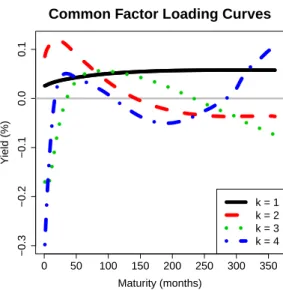
In Figure 2.2, we plot the posterior means of the common FLCs fk for

k = 1, . . . ,4. We can interpret these fk as estimates of the time-invariant un-derlying functional structure of the yield curves shared by the Fed, the BOE, the ECB, and the BOC. The FLCs are very smooth, and the dominant hump-like features occur at different maturities—following from the orthonormality con-straints—which allows the model to fit a variety of yield curve shapes. Interest-ingly, the estimated f1, f2, and f3 are similar to the level, slope, and curvature

(42)

functions of the Nelson-Siegel parameterization described by Diebold and Li (2006). Since the factors β(_k,tc) serve as weights on the FLCs fk in (2.2), we may interpret the factorsβ_k,t(c)—and therefore the slopesγ_k(c)—based on these features of the yield curve explained by the correspondingfk.

0 50 100 150 200 250 300 350 −0.3 −0.2 −0.1 0.0 0.1

Common Factor Loading Curves

Maturity (months) Y ield (%) k = 1 k = 2 k = 3 k = 4

Figure 2.2: Posterior means of the common FLCs,{f1, f2, f3, f4}, as a function of

maturity,τ.

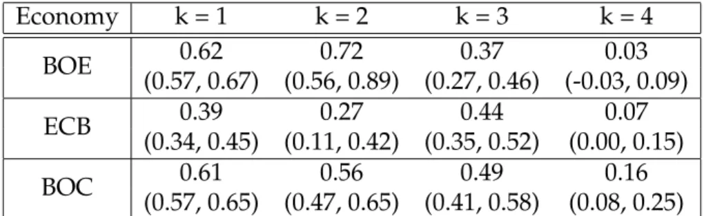
In Table 1, we compute posterior means and 95% highest posterior density (HPD) intervals forγ_k(c), which measures the strength of the linear relationship betweenβ_k,t(c) and β_k,t(1). For the level and slope factorsk = 1,2, the ECB is sub-stantially less correlated with the Fed factors than are the BOE and BOC factors. Fork = 4, the BOE, ECB, and BOC factors are nearly uncorrelated with the Fed factors.

Finally, we analyze the conditional standardized residuals from model (2.8),

rk,(c),t =

ω_k,t(c)−φ(_k,c)₁ω_k,t(c)₋₁/σk,(c),t iid

∼ N(0,1), to determine periods of time t

for which (2.8) is inadequate, which can indicate deviations from the assumed linear relationship between the Fed factors and the other economy factors. By computing the MCMC sample proportion of r_k,2₍_c₎_,t ∼ χ2₁ that exceed a critical

(43)

Economy k = 1 k = 2 k = 3 k = 4 BOE 0.62 0.72 0.37 0.03 (0.57, 0.67) (0.56, 0.89) (0.27, 0.46) (-0.03, 0.09) ECB 0.39 0.27 0.44 0.07 (0.34, 0.45) (0.11, 0.42) (0.35, 0.52) (0.00, 0.15) BOC 0.61 0.56 0.49 0.16 (0.57, 0.65) (0.47, 0.65) (0.41, 0.58) (0.08, 0.25)

Table 2.1: Posterior means and 95% HPD intervals forγ_k(c), which measures the strength of the linear relationship betweenβ_k,t(c) andβ_k,t(1).

value of the χ2-distribution, e.g., the 95th percentile χ2₁_,₀_.₀₅ ≈ 3.84, we can ob-tain a simple estimate of the probability that r2_k,₍_c₎_,t exceeds the critical value and, by that measure, is likely an outlier. We can compute a similar quantity for P4

k=1r 2

k,(c),t ∼χ

2

4, which aggregates across factorsk = 1, . . . ,4. In Figure 2.3, we

plot these MCMC sample proportions, restricted to the U.S. recession of Decem-ber 2007 to June 2009. Around NovemDecem-ber 2008, there were outliers for all three economies fork = 2,3,4and the aggregate, which suggests that the U.S. interest rate market may have behaved differently from the other economies during this time period. We are currently investigating an extension of model (2.8) to in-corporate several important financial predictors as covariates, with a particular focus on the weeks during the recession.

2.4.2

Multivariate Time-Frequency Analysis for Local Field

Po-tential

Local field potential (LFP) data were collected on rats to study the neural ac-tivity involved in feature binding, which describes how the brain amalgamates distinct sensory information into a single neural representation (Botly and De

(44)

Figure 2.3: The MCMC sample proportions ofr2 k,(c),tand P4 k=1r 2 k,(c),tthat exceed the 95th percentile of the assumedχ2_{-distributions.}

Rosa, 2009; Ljubojevic et al., 2013). LFP uses pairs of electrodes implanted di-rectly in local brain regions of interest to record the neural activity over time; in this case, the brain regions of interest are the prefrontal cortex (PFC) and the posterior parietal cortex (PPC). The rats were given two sets of tasks: one that required the rats to synthesize multiple stimuli in order to receive a reward (calledfeature conjunction, or FC), and one that only required the rats to process a single stimulus in order to receive a reward (calledfeature singleton, or FS). FC involves feature binding, while FS may serve as a baseline. The tasks were re-peated in 20 trials each for FS and FC, during which electrodes implanted in the PFC and the PPC recorded the neural activity. Therefore, the raw data signal is a bivariate time series with 40 replications for each rat; we show an example of the bivariate signals for one such replication in Figure 2.4a. Each signal replicate is 3 seconds long, and has been centered around the behavior-based laboratory estimate of the time at which the rat processed the stimuli, which we denote byt∗.

(45)

(a) The bivariate LFP signal. 0.0 0.2 0.4 0.6 0.8 −140 −135 −130 −125 −120 −140 −135 −130 −125 −120 −115 −300 −290 −280 −270 −260 −250 −240 2 4 6 8 10 12 14 10 20 30 40 50 60 70 80 Log−Spectrum, PFC Frequency (Hz) 2 4 6 8 10 12 14 10 20 30 40 50 60 70 80 Log−Spectrum, PPC Time Bin Frequency (Hz) 2 4 6 8 10 12 14 10 20 30 40 50 60 70 80 Log−Cross−Spectrum 2 4 6 8 10 12 14 10 20 30 40 50 60 70 80 Squared Coherence Time B