Wireless sensor network redeployment under the target coverage constraint

Wireless sensor network redeployment under the target

coverage constraint

Dimitrios Zorbas, Tahiry Razafindralambo

To cite this version:

Dimitrios Zorbas, Tahiry Razafindralambo. Wireless sensor network redeployment under the

target coverage constraint. [Research Report] RR-7818, INRIA. 2011, pp.16.

<

hal-00646342

>

HAL Id: hal-00646342

https://hal.inria.fr/hal-00646342

Submitted on 29 Nov 2011

HAL

is a multi-disciplinary open access

archive for the deposit and dissemination of

sci-entific research documents, whether they are

pub-lished or not.

The documents may come from

teaching and research institutions in France or

abroad, or from public or private research centers.

L’archive ouverte pluridisciplinaire

HAL

, est

destin´

ee au d´

epˆ

ot et `

a la diffusion de documents

scientifiques de niveau recherche, publi´

es ou non,

´

emanant des ´

etablissements d’enseignement et de

recherche fran¸

cais ou ´

etrangers, des laboratoires

publics ou priv´

es.

IS S N 0 2 4 9 -6 3 9 9 IS R N IN R IA /R R --7 8 1 8 --F R + E N G

RESEARCH

REPORT

N° 7818

Wireless sensor network

redeployment under the

target coverage

constraint

RESEARCH CENTRE LILLE – NORD EUROPE

Parc scientifique de la Haute-Borne 40 avenue Halley - Bât A - Park Plaza 59650 Villeneuve d’Ascq

Wireless sensor network redeployment under

the target coverage constraint

Dimitrios Zorbas, Tahiry Razafindralambo

Project-Teams POPS

Research Report n° 7818 — November 2011 — 13 pages

Abstract: A critical problem of wireless sensor networks is the efficient handling of the nodes energy under the target coverage constraint. The sensors are randomly deployed in the field covering a set of targets. Due to the randomness of the deployment some targets are covered by a few only sensors. Thus, the maximum achieved network lifetime is upper bounded by the energy of the sensors that cover the most poorly covered target. To tackle this problem one could move some sensors to these poorly covered areas from areas that are covered by many sensors. In this paper we present centralised and localised solutions that can be used to redeploy the sensing nodes and balance the amount of energy between the sensors that cover each target. We simulate our algorithms and our findings show an over 100% increase of the amount of energy of the sensors that cover the most poorly covered target in the network.

Redéploiement de réseau de capteurs contraint

par la couverture de cible

Résumé :

WSN redeployment 3

1

Introduction

Wireless sensors networks consist of hundreds of tiny nodes with limited battery lifetime. The nodes are used to monitor a number of events that periodically occur in some areas of the field called the “targets”. The nodes use their sensing range to monitor the events that may occur in a proximate target. Moreover, they use their communication range to exchange data with other nodes in the network.

Because of the randomness of the deployment, other targets may be cov-ered by a small number of sensors and others by a large number of nodes. In applications where there is the need of full coverage, the target that is covered by the lowest number of nodes, sets an upper bound on the maximum achieved network lifetime [8]. In other words, the sensors that cover poorly covered tar-gets exhaust their energy faster than the other sensing nodes in the network. This observation leads to at least one uncovered target, while other targets still remain covered by many nodes. Since the monitoring process terminates when at least one target cannot be covered anymore, the energy of the sensors that cover other targets cannot be used.

To tackle the problem above, we present two algorithms, a centralised algo-rithm and a localised one, that redeploy sensors between target areas, such that all the targets will be covered by about the same number of sensors. Specifi-cally, our algorithms take nodes from targets that are covered by many sensors and move them to more sparsely covered targets. By this way, they distribute the available energy among all the targets in the network and increase the total amount of energy that is related to the most poorly covered target.

The redeployment takes place before other operations of the network, such as the monitoring operation or the routing operation. Apparently, during the redeployment, the nodes’ movement consumes energy, so the network after the redeployment consists of less energy than before. However, this amount of energy is spent by the sensors that cover richly covered targets and without the redeployment process their energy would remain useless.

An important requirement of a sensor network is the connectivity with the sink. Making the assumption that initially all the sensing nodes are connected with the sink using neighbouring relay nodes, the final network will remain connected as well. This statement holds true, since the nodes are moved only from a target to another target and no relay node changes position. In the case where there is an insufficient number of relay nodes, redeployment cannot guarantee connectivity and a relay node redeployment is needed. This paper focuses on sensing node redeployment leaving this special case for consideration in our future work.

The rest of the paper is organised as follows. In Section 2, we present the related work in the fields of target coverage and mobile sensor networks. In Section 3, we provide a formal description of our problem, while in Section 4 we present our two solutions. In Section 5 we evaluate our methods and we compare them to the case where the nodes are non-mobile. Finally, Section 6 concludes the paper.

4 Zorbas & Razafindralambo

2

Related work

Most of the works about target coverage in WSNs deal with the problem of dividing the available sensors in sets, such that only one set is active at any time [2, 7, 8]. By successively activating the sets, the network lifetime can be increased. In [8] a special care is taken for the sensors cover poorly covered targets, when the monitoring data of each sensing node are forwarded to the sink. However, these works assume static nodes and the maximum achieved network lifetime still depends on the initial number of sensors cover the most poorly covered target in the network.

From the other hand, the works that deal with sensor redeployment consider only the case of the uniform coverage of a large monitored area [6, 5, 3, 4]. The algorithms presented in these works are basically based on the use of virtual forces or voronoi diagrams, where each node pushes its neighbours to more sparsely covered areas. However, these algorithms cannot be used in the target coverage problem, since they require a continuous deployed area (not only the area around each target) in order to provide a uniform area coverage.

3

The Target Coverage Redeployment Problem

LetT0 ={t1, t2, . . . , tk} be the set of targets and S0={s1, s2, . . . , sn} the set

of sensors. Initially, each target inT0is covered by at least one sensor inS0if it

is in a sensor’s sensing rangeRs. Each sensor has a maximum communication

rangeRc and an initial battery lifetime equal tol0. A sensor may spend a part

of this energy to move itself to another location. This amount of energy depends on the distance and it is equal toαm. Moreover, letlj be the energy of a sensor

sj throughout the redeployment process.

Set N = {N1, N2, . . . , Nk} contains the sets of sensors that each target is

covered by. navg is the average number of sensors that cover a target among all

the targets and it is given by:

navg=

|N1|+|N2|+. . .+|Nk|

k , (1)

where|Ni|is the cardinality ofNi,i∈[1, k]. LetN′ contain the sets of sensors

that each target is covered by after the redeployment process.

The objective of the redeployment algorithm is to solve the Target Cover-age Redeployment Problem (TCRP) by achieving min(|N1′|,|N2′|, . . . ,|Nk′|) =

⌊navg⌋, and maximise

|N′

min|

X

j=1

lj, subject to lj >0 ∀ sj ∈S0, where tmin is the

target covered by the lowest number of sensors at the end of the redeployment. InN′ _{the most poorly covered target is defined as the target that the sum}

of the energy of the sensors covering this target is less than or equal to the sum of the energy of the sensors covering each of the other targets in the network.

If we consider a constant energy consumption per meter, the maximum dis-tance that a node is able to be moved isdmax=_αl0_m. Since a sensor is moved from

a target area to another target area, the maximum distance that two targets can be found, in order to exchange sensors, is equal todmax. This practically

means that if a sensor is equipped with two AA-type batteries and consumes

WSN redeployment 5

100J/mto move itself, then the maximum distance between two targets will be 141 meters. In other words, the maximum allowed size of a square-shaped terrain would be 20,000m2_.

4

Solutions for TCRP

In this section we present two solutions to solve TCRP. The first one is a cen-tralised algorithm that has a complete knowledge of the parameters of the net-work; the location of the nodes, the location of the targets and the distances between them. The second one is a localised solution where the nodes decide if, who and where a sensor may be moved. According to this solution each node does not have a complete knowledge of the network, but it initially knows its own location and the coordinates of the targets.

Greedy-TCR (see Algorithm 1) is a centralised algorithm that begins by computingnavg and the sharing factor (i.e. sf) for each target in the network

(Step 1). The sharing factor shows how many sensors may offer or receive a particular target by other targets in order to decrease or increase the number of sensors that is covered by. In Step 2, each target that can receive nodes computes a number of distances to sensors that cover targets with redundant nodes. This number of sensors depends on how many nodes the target-donator is covered by. Greedy-TCR keeps these distance in a temporary setDalong with the target-receiver, the target-donator and the sensor that may be moved. All these distances are examined in Step 3 and the shortest distances are selected. The sharing factors of the targets are updated respectively.

Since no other node can be moved, Greedy-TCR moves the selected sensors to the appropriate location. Each sensor moves on the straight line between its initial location and the receiver. It stops when the distance to the target-receiver is equal to Rs. Greedy-TCR checks if the target-receiver is the only

target that can be covered from this location. If not, Greedy-TCR avoids to cover multiple targets using a single sensor, a fact that could affect the sharing factor of some other targets and could lead to infinite number of movements. Thus, the node is moved to a place that can cover only the target-receiver. If the energy consumption due to the movement is higher than the available energy of the sensor, the algorithm abandons this movement and continues with the next sensor.

Even if no other sensor can be moved due to the restrictions on the selection of the distances (e.g. a node has no available energy), some targets may still remain covered by a higher number of sensors thannavg. Greedy-TCR, in Step

4, finds the target surrounded by the minimum amount of energy among all the targets and moves towards it the closest node to this target. These nodes had not been tested during Step 2, because other sensors where closer to the target-receivers. Greedy-TCR ends by returning setN′_.

Greedy-TCR may not provide always the optimal solution (i.e. the minimum total traveling distance). In order to find the optimal result an algorithm should check among n₂! possible solutions inheriting a prohibitive complexity. The longest run of Greedy-TCR appears when all the targets take part in Step 2 of the algorithm. Thus, the complexity of Greedy-TCR isO(k2n), wherekis the number of targets andnthe number of sensors.

Local-TCRis a distributed and localised algorithm that operates in rounds.

6 Zorbas & Razafindralambo Algorithm 1:Greedy-TCR require:S06=∅,Ni6=∅,∀ti∈T0,T06=∅,l0>0 // Step 1 navg= |N1|+|N2|+...+|_Nk| k ; foreacht∈T0do if |Nt|> navgthen sft=⌊|Nt| −navg⌋; else sft=⌈navg− |Nt|⌉; // Step 2 D=∅; foreacht∈T0do if sft<0then foreacht′_∈T 0do ifsft′ >0then

select thesft′ shortest distances fromtto a sensorsj that coverst′; keep these distances inDalong witht,t′andsj;

// Step 3

moving_nodes=∅;

whileno node can be moveddo foreachd∈Ddo

select the shortestd;

sft=sft+ 1;

sf_t′=sf_t′−1;

marksj as a moving node;

foreachsj∈moving_nodesdo

movesj to the appropriate location and updatelj;

// Step 4

Repeat Step 1;

foreacht∈T0do

if sft>0then

compute targett′surrounded by the minimum amount of energy; find the sensorsjthat coverstand it is in the shortest distance tot′; movesj tot′;

returnN′_;

In each round (see Algorithm 2) the sensing nodes perform a number of opera-tions to decide which nodes will be moved from a target area to another. During the first operation each node covering a target discovers the neighbouring nodes that also cover this particular target. Each node keeps this set of neighbouring sensors in its memory, excluding those that cover other targets at the same time. Along with the neighbour set, a node is able to buildnifor eachtiit monitors.

niis named “target cardinality” and represents the number of sensors that cover

ti (i.e. ni is equal to|Ni|).

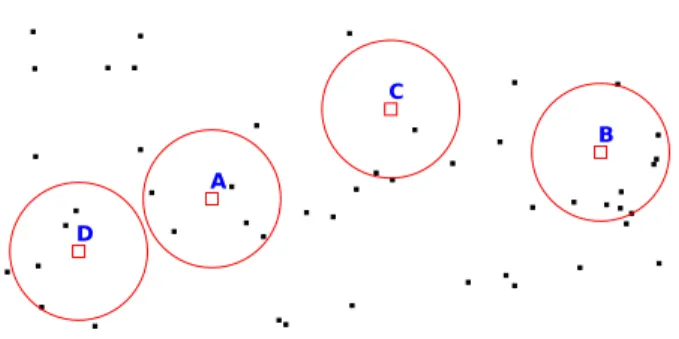
In Figure 1 a network consists of four targets (squares) and a number of sensing nodes (dots) covers these targets. All the nodes that are between the circle and the target, can monitor this particular target and consistni of target

ti (i.e. nA= 5,nB = 8, nC= 2andnD = 4). The radius of the circle is equal

toRs.

Since all nodes know their neighbours and how many other sensors cover their covered targets, they can compute their sharing factor. To do this, each par-ticular node receives the corresponding cardinalities of the neighbouring nodes; the nodes that are in its communication range and cover different targets than what the particular node covers. In Figure 1, supposing that the communica-tion range is about 5 times the sensing range, a node that covers target “B” can

WSN redeployment 7

Figure 1: A network with 4 targets

directly communicate with nodes covering target “C” and nodes covering target “A”, but not with nodes covering target “D”.

Each particular node computes a local sharing factor of the cardinalities of the targets that it covers along with the cardinalities of the targets that the neighbouring nodes cover. The cardinalities that are larger or equal to the average cardinality of the targets that the particular node covers, are not taken into account in this computation. Depending on the value of the local average, a node can offer (supporter) or receive nodes (receiver) for the targets it covers. Each supporter keeps in its memory the closest receivers for each target it supports. In Figure 1, a node that covers target “A” computes a sharing factor equal to⌊nA−nA+n₃D+nC⌋= 1. nB is not taken into account, because

nB> nA. So, nodes covering “A” can be supporters for this round.

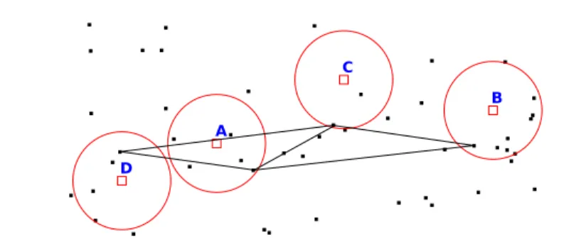
During the next phase, each supporter receives the sharing factor of all the other supporters in the network. This operation is needed in order to avoid having two different supporters sending sensors to the same receiver. To avoid flooding of the network, one or more head-nodes are assigned for each target and a backbone network is built. This backbone network consists of head-nodes that may be supporters or receivers. A supporter can be head of a targetti if

there is no other node inNi closer to a neighbouring target. Supporters that

are not head-nodes can receive the sharing factors of the other supporters in the network through their target head-node. The lines illustrated in Figure 2 correspond to the backbone paths.

Since all supporters have the sharing factor of the other ones, they compare it with their own. The node with the highest sharing factor is allowed to de-cide who, where and how many nodes will be moved. This node is called the “leader”. In order to avoid having two leaders in the same round, nodes multiply their sharing factor with a random value in(1,1.01]before send it to the other supporters. For example, a node covering target “B” will be the leader in Figure 1.

During the last phase, the leader finds the receiver that needs the highest number of sensors and computes how many nodes could offer it. The number of nodes that will be moved, let sayf, is equal to⌊max(ns1, . . . , nsk)−min(nr1, .., nrl)

2 ⌋,

where ts1, . . . , tsk are the targets covered by the supporter and tr1, . . . , trl are

the targets covered by the receiver. The leader looks in the set of neighbouring nodes for thef closest nodes to the target-receiver. In case that its own distance is shorter than at least one of the otherf nodes, it can move itself excluding one of the otherf nodes. Since the moving nodes have been discovered, the leader

8 Zorbas & Razafindralambo

Figure 2: Head-nodes and backbone paths of the network

computes their final destination similar to the centralised algorithm. The next round starts when the nodes have reached their final destination. In the exam-ple of Figure 1, the two left nodes of target “B” will be moved, since they are closer to target “C”. The new location of these two nodes is indicated by a circle in Figure 3.

Theorem 1. Local-TCR always balances the number of monitoring nodes be-tween two neighbouring targets when the number of nodes covering the two tar-gets differs by two or more sensors.

Proof. Since all the nodes covering these two targets have built the set of neigh-bouring nodes and the cardinality sets, they are ready to compute their sharing factor. Lettµ and tλ be the two targets, wherenµ−nλ ≥2. Let alsosµ and

sλ be two sensors that covertµ andtλ, respectively. The sharing factors of the

two sensors will be:

sfsµ =⌊nµ− nµ−nλ 2 ⌋=⌊ nµ−nλ 2 ⌋, and sfsλ =⌊nλ− nλ 1 ⌋= 0.

This practically means that sµ will move at mostf =⌊nµ−₂nλ⌋nodes towards

tλ in Phase 5. In order to have a balanced final network, it should be true that

n′

µ−n′λ ≤1. It is true thatn′µ = nµ−f and n′λ =nλ+f. It follows that

nµ−f−nλ−f ≤1which is equal tonµ−nλ≤1 + 2f. Usingnµ−nλ≥2, it

follows thatf ≥1

2, which is true becausef is integer andf ≥1.

In the very special case where three successive targets are covered by k1,

k2 and k3 sensors respectively, andk1−k2 = 1and k2−k3 = 1, Local-TCR

will fail to balance the number of sensors between t1 and t3. This problem

could be solved by allowing the sensors to receive the coverage status of their 2-hop neighbouring nodes in the network during Phase 2. However, this would increase the total overhead of the network.

5

Evaluation and discussion of the results

In this section we simulate the proposed algorithms and we compute the amount of energy of the sensors cover the most poorly covered target. We compare the results to the case where the nodes are static and cannot be moved.

We assess the algorithms in 50 topologies with random and uniform target and sensor deployments and we compute the average energy value of these 50

WSN redeployment 9

Figure 3: New location of the nodes moved

topologies. The 95% confidence intervals are shown in each figure. The commu-nication range of the nodes is50mand their sensing range is10m. We assume that two targets cannot be found in a distance shorter than the sensing range. The battery of the sensors is initially equal to 20KJ (this is a typical energy capacity of one C-type or two AA-type batteries [1]). A sensor consumes 100

Joules of energy in order to travel one meter distance, except from the last scenario where the energy consumption varies.

5.1

Simulation results

The first scenario involves 60 deployed sensors and 15 targets scattered on a ter-rain with variable size. Varying the terter-rain size we assess the algorithms on the network density. The results presented in Figure 4 show an over 100% increase on the energy corresponds to the most poorly covered target in comparison to the case where the nodes cannot be moved (i.e. Wo redeployment). As it was expected, the minimum energy decreases as the terrain size increases and less sensors are able to monitor the targets. The centralised algorithm performs a little bit better than the localised algorithm, as it has a complete knowledge of the network and can move sensors between distant targets minimising the total traveling distance.

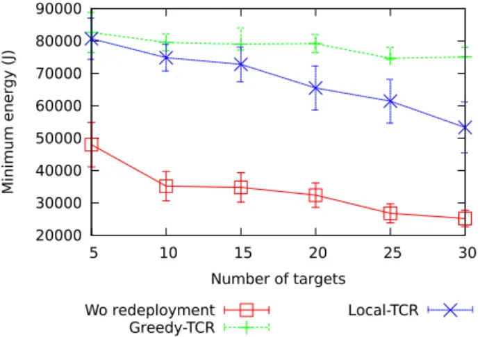
In Figure 5 is shown the performance of the algorithms in a scenario with constant number of sensors and fixed terrain size. We gradually increase the number of targets from 5 to 30. The two algorithms improve a lot the total amount of energy of the sensors that cover the most poorly covered target, but the centralised algorithm performs better than the localised when many targets are deployed. As in the previous scenario, this occurs due to the fact that the localised algorithm moves sensors only between neighbouring targets and, thus, some sensors travel longer distances to move to a distant target. When the number of targets is higher, the number of movements is increased and the nodes consume more energy.

In the next scenario, we evaluate the algorithms in the case where the num-ber of targets remains constant in a fixed-size terrain with variable numnum-ber of sensors. The findings are illustrated in Figure 6 and show a high increase in cases where the number of sensing nodes is above 40. When a few only nodes are deployed the improvement is small due to the fact that the most of the targets are covered by one or two nodes. However, in all the cases, the localised algorithm remains very close to the centralised approach.

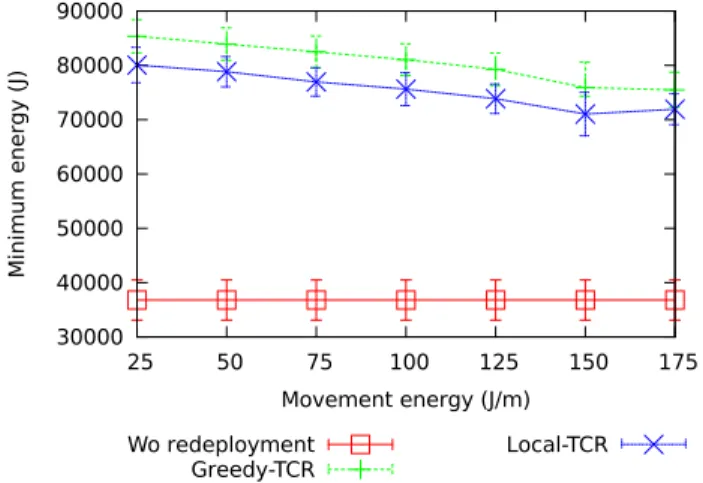
Finally, in the last scenario, we vary the energy consumption yielded by a

10 Zorbas & Razafindralambo Algorithm 2:Local-TCR require:S06=∅,T06=∅,l0>0 // Phase 1 foreachs∈S0do neighbouring_sets=∅; foreachs′ in communication range ofsdo if s′_∈S

0and covers the same targetsthen

neighbouring_sets=neighbouring_sets∪ {s′};

foreachs∈S0do

foreachtin sensing range ofsdo

nt= 1;

foreachs′in communication range ofsdo ifs′_∈S

0and coverstthen

nt=nt+ 1;

// Phase 2

foreachs∈S0do

foreachtin sensing range ofsdo

sfs=sfs+nt;

sfs′=sfs/(# of targets in sensing range ofs);

foreachs′

in communication range ofsdo

if s′∈S0then

foreacht′ _{in sensing range ofs}′_do

ifnt′ < sfs′ then

sfs=sfs+nt′;

sfs=sfs/(# of covered and examined targets);

sfs=⌊(max(ns1, ..., nsk)−sfs)⌋; if sfs>0then sis supporter; else if sfs= 0then sis receiver; // Phase 3 foreachsupportersdo can_supports=∅;

foreachreceivers′in communication range ofsdo

can_receive_s′ =∅;

foreachtin sensing range ofs′_do

ifs′ is in the closest distance tosthen

can_supports=can_supports∪ {t};

can_receives′ =can_receives′∪ {s};

ifno other node inneighbouring_sets is closer tos′ then makesands′head-nodes;

// Phase 4

foreachsupportersdo

receive the sharing factor of the other supporters (multiplied by a random number in (1,1.02]);

compute the max sharing factorsfmaxthat you have received;

if sfs> sfmaxthen

sis the leader;

// Phase 5 (operations by leader s)

f=⌊max(ns1, . . . , nsk)−min(nr1, .., nrl)

2 ⌋;

find thefclosest nodes to the target-receiver;

move this nodes to the target-receiver if they have available energy;

node’s movement. We keep constant the other parameters of the network. The results illustrated in Figure 7 show that even in the case where the energy con-sumption is large, both Greedy-TCR and Local-TCR can increase the amount

WSN redeployment 11

! " #$

% & " #$

Figure 4: Total amount of energy of the sensors covering the most poorly covered target (minimum energy) in a scenario with 60 nodes, 15 targets and a variable terrain size

!" # $%&'

( ) "$%&'

Figure 5: Total amount of energy of the sensors covering the most poorly covered target (minimum energy) in a scenario with 60 nodes, 10Km2 _{terrain size and}

variable number of targets

of energy that corresponds to the most poorly covered target.

6

Conclusion and future work

In this paper we dealt with the redeployment of a set of sensors that cover a number of targets in the field. Since the nodes are randomly deployed, sensors that cover the most poorly covered target set an upper bound on the network lifetime. To tackle this problem, we presented two algorithms that balance the number of sensors between the targets. The first algorithm works centralised and has a complete knowledge of the network parameters. The second one is a localised solution that is based on the neighbouring information. The evaluation results showed that the energy of the sensors that cover the most poorly covered

12 Zorbas & Razafindralambo

!"

# $% !"

Figure 6: Total amount of energy of the sensors covering the most poorly covered target (minimum energy) in a scenario with variable number of nodes, 15 targets and 10Km2_{terrain size}

!"#$

% &' !"#$

Figure 7: Total amount of energy of the sensors covering the most poorly covered target (minimum energy) in a scenario where we vary the movement energy consumption

target can be doubled by applying one of the previous redeployment approaches. Since connectivity is an important requirement of a sensor network, we are working on providing a scheme that ensures connectivity, even in the case where the network is not initially connected.

References

[1] Battery energy storage.http://www.allaboutbatteries.com/Energy-tables.html. [2] Ionut Cardei and Mihaela Cardei. Energy efficient connected coverage in

wireless sensor networks. Int. J. Sen. Netw., 3(3):201–210, 2008.

WSN redeployment 13

[3] Nojeong Heo and P.K. Varshney. Energy-efficient deployment of intelligent mobile sensor networks. Systems, Man and Cybernetics, Part A: Systems and Humans, IEEE Transactions on, 35(1):78 – 92, jan. 2005.

[4] Foued Kribi, Pascale Minet, and Anis Laouiti. Redeploying mobile wireless sensor networks with virtual forces. InProceedings of the 2nd IFIP confer-ence on Wireless days, WD’09, pages 254–259, Piscataway, NJ, USA, 2009. IEEE Press.

[5] Guiling Wang, Guohong Cao, and T. La Porta. Proxy-based sensor deploy-ment for mobile sensor networks. In Mobile Ad-hoc and Sensor Systems, 2004 IEEE International Conference on, pages 493 – 502, oct. 2004. [6] Guiling Wang, Guohong Cao, and Thomas F. La Porta. Movement-assisted

sensor deployment. IEEE Transactions on Mobile Computing, 5:640–652, June 2006.

[7] Qun Zhao and Mohan Gurusamy. Lifetime maximization for connected target coverage in wireless sensor networks. IEEE/ACM Trans. Netw., 16(6):1378–1391, 2008.

[8] Dimitrios Zorbas and Christos Douligeris. Connected coverage in wsns based on critical targets. Computer Networks, 55(6):1412 – 1425, 2011.

Contents

1 Introduction 3

2 Related work 4

3 The Target Coverage Redeployment Problem 4

4 Solutions for TCRP 5

5 Evaluation and discussion of the results 8

5.1 Simulation results . . . 9

6 Conclusion and future work 11

RESEARCH CENTRE LILLE – NORD EUROPE

Parc scientifique de la Haute-Borne 40 avenue Halley - Bât A - Park Plaza 59650 Villeneuve d’Ascq

Publisher Inria

Domaine de Voluceau - Rocquencourt BP 105 - 78153 Le Chesnay Cedex inria.fr