Alma Mater Studiorum
Alma Mater Studiorum –
– Università di Bologna
Università di Bologna
DOTTORATO DI RICERCA IN
SCIENZE STATISTICHE
Ciclo XXIX
Settore Concorsuale di afferenza:13/A5
Settore Scientifico disciplinare: SECS-P/05
ESSAYS IN THE ECONOMETRIC ANALYSIS
OF SYSTEMIC RISK MEASURES
Presentata da: Alice Monti
Coordinatore Dottorato
Relatore
Prof. Alessandra Luati
Prof. Giuseppe Cavaliere
Correlatore
Prof. Christian Brownlees
Contents
1 Introduction 1
1.1 Systemic risk: definition and measurement . . . 1
1.2 Motivation and overview . . . 4
2 Systemic Risk review 9 2.1 Systemic Risk measures . . . 9
2.1.1 CoVaR-based Systemic Risk measures . . . 11
2.1.2 MES-based Systemic Risk measures . . . 16
2.1.3 Alternative probability-distribution measures . . . 20
2.1.4 Network Analysis measures . . . 26
2.2 Econometric models for Systemic Risk . . . 28
2.2.1 GARCH model . . . 29
2.2.2 GJR model . . . 31
2.2.3 DCC model . . . 32
2.3 Concluding remarks . . . 37
3 Systemic Risk evaluation 39 3.1 Related literature on backtest . . . 40
3.1.1 Unconditional coverage test . . . 42
3.1.2 Independence test . . . 43
3.1.3 Correct conditional coverage test . . . 44
3.2 Related literature on test and loss function . . . 44
3.2.1 Conditional volatility evaluation . . . 45
3.2.2 Tick loss function . . . 46 iii
3.2.3 Dynamic quantile test . . . 47
3.2.4 Magnitude loss function . . . 48
3.3 A new approach to evaluate tail forecasts . . . 49
3.3.1 New loss functions in CoVaR framework . . . 49
3.3.2 New loss functions in MES framework . . . 51
3.4 Concluding remarks . . . 52
4 Empirical study of 2007−2009 crisis 55 4.1 US financial data . . . 55
4.2 In-sample estimation . . . 58
4.3 Out-of-sample forecast . . . 63
4.3.1 Sub-samples comparison . . . 66
4.4 Concluding remarks . . . 67
5 Econometric modeling of long-range dependence in Systemic Risk mea-surement 69 5.1 Related literature . . . 70
5.1.1 Component-GARCH model . . . 71
5.1.2 Spline-GARCH model . . . 74
5.1.3 FIGARCH model . . . 76
5.2 A new Asymmetric-Component-GARCH model . . . 77
5.2.1 Model Specification . . . 78 5.2.2 Forecasting . . . 79 5.3 Empirical analysis . . . 79 5.3.1 In-sample estimation . . . 80 5.3.2 Out-of-sample forecast . . . 89 5.3.3 Sub-samples comparison . . . 95
5.3.4 Case-study: Bank of America . . . 98
5.4 Concluding remarks . . . 98
6 Conclusions 101
CONTENTS v Appendices
A The empirical measures 119
A.1 Empirical CoVaR measure by Adrian and Brunnermeier . . . 119
A.2 Empirical CoVaR measure by Girardi and Ergun . . . 120
A.3 Empirical MES measure . . . 122
A.4 Algorithm procedure for empirical measures . . . 122
Abstract
This thesis aims at the study of systemic risk measurement, which became crucial after the 2007−2009financial crisis. The objective of the thesis is twofold: (i) we address the issue of assessing the accuracy of systemic risk measures, (ii) we investigate the role of the long-range dependence in systemic risk forecasting, under both methodological and em-pirical perspectives. From the methodological point of view, we propose two appropriate loss functions, the Tail Tick Loss function and the Tail Mean Square Error, specifically designed to evaluate the CoVaR and MES accuracy, respectively. Moreover, we introduce a comprehensive model called Asymmetric-Component-GARCH (ACGARCH), which is able to capture both the leverage effect and long-range dependence. An empirical analysis of different bivariate volatility models to the daily returns of91US financial institutions in the period 2000−2012 confirms the need of employing appropriate loss functions to evaluate systemic risk accuracy and to discriminate among different competing models. Moreover, empirical results encourage the usage of the ACGARCH model in the systemic risk framework.
Acknowledgements
I would like to thank my supervisor Prof. Giuseppe Cavaliere for accepting me as PhD student and for giving me the chance to learn from him. I express my sincere gratitude to my co-supervisor Prof. Christian Brownlees for the great support and the very relevant research experience I did as visiting PhD student in Barcelona. Thanks to all my research group for the useful comments and support. In particular, I am grateful to Prof. Michele Costa for precious advices, to Prof. Iliyan Georgiev for extremely useful suggestions and, last but not least, to Dr. Luca De Angelis for all his support during the all PhD. Many thanks to my family for teaching me to never give up, for giving me the opportunity to chase my passions and for believing always in me. A special thanks to Alessandro for bearing and sharing tough moments and stressful periods. This PhD experience has enriched me from both human and educational perspectives and I am very glad to have completed this journey.
Chapter 1
Introduction
This chapter explains systemic risk, whose a single definition is not shared in the litera-ture, motivating the importance of its measurement for the society. How to define and measure it is the object of interest over the last years, however it is still an open issue. After providing an overview over the existing definitions and different approaches’ points of view, the motivation and the structure of the thesis work are presented.
1.1
Systemic risk: definition and measurement
The 2007−2009 financial crisis developed the need of measuring systemic risk for the whole economy with the purpose to evaluate the vulnerability of the financial system and the risk of different financial institutions on the whole market, since a single institution’s risk measure does not necessarily reflect systemic risk (e.g. Value-at-Risk). The failure of big financial institutions infected the entire financial system and even brought severe consequences to the real economy on a global scale, such as the bankruptcy of Lehman Brothers, which demonstrated the fragility of the whole financial system. Furthermore, through the spillovers from the financial system to the real economy, which drops into a deep recession, and through the bailouts of big companies with taxpayers’ money, finan-cial crises impose high costs for the society, leading to consider managing systemic risk as a desirable goal.
In the light of the global financial crisis and due to the acknowledgement of the impor-1
tance of systemic risk, several organisms were created in order to control and supervise the stability of the financial system. Among the others, the U.S. Congress, in 2010, created the Office of Financial Research (OFR), and European Systemic Risk Board (ESRB) was born in April 2009 in order to ensure financial stability. Finally, regulators have been given a mandate to measure and monitor systemic risk.
The precise definition of systemic risk is still ambiguous and many proposals are present in the literature. Billio et al., in 2012, specify systemic risk as “any set of circumstances that threatens the stability of or public confidence in the financial system”, whereas the European Central Bank (ECB), in 2010, defines it as a risk of financial instability “so widespread that it impairs the functioning of a financial system to the point where economic growth and welfare suffer materially”. Daniel Tarullo, the Federal Reserve Governor, in2009, states that “Financial institutions are systemically important if the failure of the firm to meet its obligations to creditors and customers would have significant adverse consequences for the financial system and the broader economy”. Finally, Acharya et al., in 2010, claim that systemic risk is the risk of a crisis in the financial sector and its spillover to the economy at large.
Systemic risk may easily be confused with systematic risk, also known as market risk or undiversifiable risk. Systematic risk is the risk explained by factors that influence the economy as a whole, and, in a portfolio, can’t be diversified. Systemic risk is, instead, more complex and, according to Staum (2012), is composed by different risks: the systematic risk and those risks deriving from several financial market phenomena, such as contagion, spillover, transmission of losses and distress from one institution to another one. Contagion can take several forms, and, in asset pricing, it is defined as when an institution’s sale of assets into an illiquid market can cause a decline in asset prices and, thus, losses to others.
During the last decade, after that the global financial crisis highlighted the impor-tance, and boosted the development, of detailed study of systemic risk, several measures have been developed and proposed in the literature from regulators, researchers and practitioners points of view and different models have been used to estimate them ac-cording to their structure. Bisias et al., in 2012, survey not exhaustively systemic risk measures and the conceptual frameworks, describing that “when leverage is used to boost
1.1 Systemic risk: definition and measurement 3
returns, losses are also magnified, and when too much leverage is applied, a small loss can easily turn into a broader liquidity crunch via the negative feedback loop of forced liquidations of illiquid positions cascading through the network of linkages within the financial system”. In measuring systemic risk, the authors state that it is fundamental to develop a conceptual framework in a coherent fashion, and to collect and access the correct types of input-data required by the specific adopted measure.
On the contrary, Brunnermeier and Oehmke, in 2013, survey the literature on bub-bles, financial crisis and systemic risk, explaining that systemic risk builds up in the background during the run-up phase of imbalances or bubbles and it materializes only when the crisis explodes (crisis phase). As a consequence, spillover and amplification ef-fects determine the overall damage to the economy. The crisis phase starts when a trigger event occurs, whose negative effect on the financial system and real economy is ampli-fied through several channels. Research conducted on quantitative methods relating to financial stability are generally classified into three categories:
• Early Warning Indicators (EWIs), which estimate the probability of the trigger event, like bubbles;
• systemic risk measures, which evaluate the vulnerability of the financial system;
• macro stress tests, which evaluate the effects of predetermined stress scenarios on the financial system.
Stress tests are standard devices used to determine the capital that an institution will need to raise if there is a financial crisis. Regulators have to conduct stress tests every year in the United States.
Systemic risk measures attempt to capture the total and marginal risk contributions of different financial institutions on the whole market. Therefore, they are related to firm-level risk measures, which become important given the implementation of Basel II bank regulations. The purpose of these firm-level risk measures is to reduce a vast amount of data to a meaningful single statistic that summarizes risk. Risk measures for individual financial institutions, however, are typically not good systemic risk measures, since their sum does not capture the systemic risk. The sum of all risk contributions, in fact, should be equal to the total systemic risk and each one should incentivize financial
institutions to (marginally) take on the appropriate amount of systemic risk. Therefore, it becomes crucial to develop a systemic risk measure for the whole economy and a way to allocate this systemic risk across the financial institutions. Furthermore, Systematically Important Financial Institutions (SIFIs) should be individually identified by systemic risk measure, since they could cause negative risk spillover effects on others due to their interconnectedness (Brunnermeier and Oehmke, 2013).
Ellis et al., in2014, claim that “the diversity within the financial system also supports the fact that a single measure of systemic risk is unlikely to be universally applicable, nor is a single instrument of financial stability policy”. Again, according to Hattori et al. (2014), using only systemic risk measures is not sufficient to assess financial stability as a whole, because systemic risk measures are silent on the loss caused by other trigger events or the probability of such black swan events. Hattori et al. (2014) suggest to use a combination of several quantitative tools to monitor and evaluate the financial system completely and comprehensively, such as EWIs, systemic risk measures and macro stress tests.
Furthermore, the difficulty of measuring systemic risk concerns another aspect. Cerutti et al., in 2012, face the problem of scarcity of data that capture the international di-mensions of systemic risk and claim that market price-based indicators are not always reliable risk measures. The global crisis has shown the important role played by financial linkages and channels of propagation, which require many not (yet) available data to be identified. The authors also report some examples which demonstrate that many aspects of global systemic risk simply cannot be captured using existing data, adding that the institutional infrastructure for global systemic risk management is inadequate or simply non-existent.
As a conclusion, measuring systemic risk is still an open issue, not yet solved.
1.2
Motivation and overview
The purpose of this work is to study how systemic risk can be measured, modeled, evaluated and compared. Our contribute to the existing literature is twofold.
1.2 Motivation and overview 5
is a key step towards the definition of a precise systemic risk measure. We focus on two of the most widespread systemic risk measures, namely∆Conditional-Value-at-Risk (∆CoVaR) (Adrian and Brunnermeier, 2011) and SRISK (Brownlees and Engle, 2015). Given the lack of statistical tools to compare them because of their economic nature, we analyze their straightforward main components, called Conditional-Value-at-Risk (here-after CoVaR) and Marginal Expected Shortfall (here(here-after MES). Therefore, we propose two new loss functions, one appropriate for each measure, with the purpose to test and compare the CoVaR and MES forecasting performances. We are also able to detect the most reliable models to predict CoVaR and MES measures, respectively.
Second, we investigate the stylized facts of financial data not captured by the standard models widely used in the literature, in particular we notice that financial data present long-range dependence. Given the lack of application of long-range dependence models in systemic risk framework, we propose a novel econometric model, in order to improve systemic risk estimation and forecasting. Thus, we contribute to the existing literature by defining, studying and applying a new model which combines in capturing leverage effect and long-range volatility dependence.
The thesis work is organized as follows. We start, in Chapter 2, with a review of the main systemic risk measures present in the literature and we continue revising the main widely used econometric models to compute them. In particular, we focus on the methodology composed by Generalized Autoregressive Conditional Heteroskedasticity (GARCH) approach for time-varying volatility (Bollerslev, 1986) and Dynamic Condi-tional Correlation (DCC) approach for time-varying correlation (Engle, 2002), called DCC-GARCH-type model.
The urgent need of measuring systemic risk, after the global financial crisis, leads to a huge availability of measures and models without providing comparisons or tools in order to discriminate them. Statistical tools designed to test and compare systemic risk forecasts, in fact, have not been properly developed, and a deep analysis on their accuracy has largely unexplored. As a consequence, a regulator or a practitioner, who has to compute systemic risk for its financial institution, for example, is in difficulty in identifying and choosing the measure and the related model to use to estimate and forecast systemic risk. Under this basic idea, considered as our first contribution to the
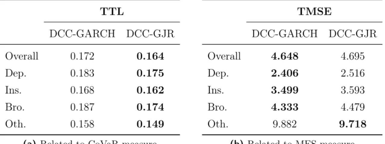
existing literature, we review, in Chapter 3, the main backtests, used to evaluate the adequacy of systemic risk measures, and the existing loss functions, used to evaluate the accuracy of risk measures, with the purpose to identify those adaptable to be used in systemic risk framework. Focusing on the accuracy, we modify and adapt these selected loss functions according to the specific systemic risk measure considered. Therefore, we develop, in Section 3.3, two new loss functions specifically designed for the CoVaR and MES frameworks, namely Tail Tick Loss and Tail Mean Square Error loss functions, respectively.
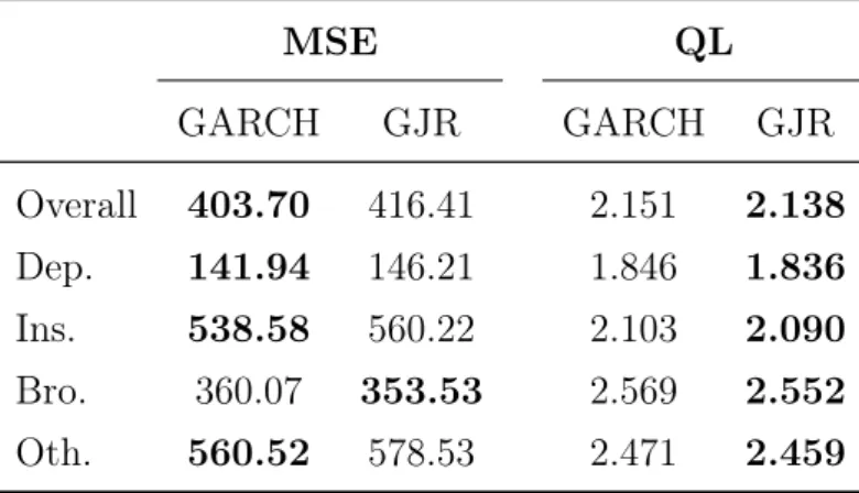
We then conduct, in Chapter 4, an empirical study of the 2007−2009 US financial crisis based on the application of DCC-GARCH-type models. We consider daily equity data of91 top US financial institutions, used by Brownlees and Engle (2015), which are all large capitalization Blue Chip companies as of end of June 2007. The dataset covers the period from January3rd2000 to December31th2012. We divide the sample period into two sub-samples in order to estimate systemic risk measures in the first sub-sample period and to forecast them in the second one. For comparative purposes, we consider the widely used quantile regression and linear regression models as benchmarks. Hence, applying the new loss functions developed in the previous Chapter, we compare the forecasting performances obtained by the benchmark and DCC-GARCH-type models, which take into account also the leverage effect present in financial data.
However, the topic is challenging and the difficulty to develop a systemic risk measure able to capture the entire nature of systemic risk with the purpose to avoid that financial institutions’ failures boost consequent failures of other financial institutions by contagion is high. Empirical results, shown in Chapter 4, go in this direction and indicate criticizes in capturing systemic events during2000−2012years. These findings lead us to explore, and then include within the methodology, other stylized facts of financial data, in par-ticular the long-range dependence in volatility, considered as our second main contribute to the existing literature, that is not yet applied in systemic risk framework. In Chap-ter 5, we then illustrate the existing econometric models that capture the long-range dependence in volatility and we propose a novel model, called Asymmetric-Component-GARCH (ACAsymmetric-Component-GARCH), able to capture both the leverage effect and long-range depen-dence in financial data. We apply the ACGARCH and existing models to the same
1.2 Motivation and overview 7
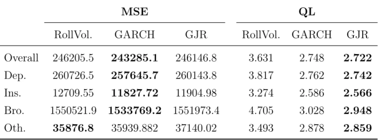
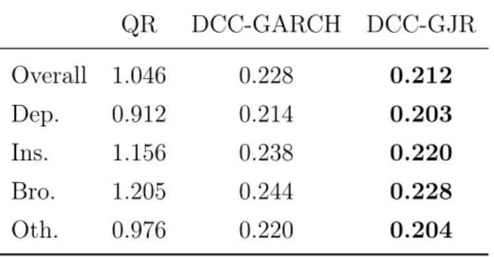
dataset used in Chapter 4, and the empirical results confirm our intuition of including long-range dependence. Moreover, using the new loss functions outlined in Section 3.3, we are able to detect the more suitable specification for the volatility that systemic risk framework requires.
Finally, Chapter 6 concludes the thesis work summing up the issues, our contributions and our findings.
The structure of all chapters is the same. They begin with an introduction part to the considered problem and they end with a concluding remarks section. Moreover, Chapters 3 and 5 provide our proposals connected to the considered issue.
Chapter 2
Systemic Risk review
An overview of the existing financial and econometric literature of measuring systemic risk is now presented. During the last decade, several systemic risk measures has been proposed in the literature from different point of views, such as probability-distribution measures, network measures, deriving both from the principal component analysis and from the graph theory. A special focus is on CoVaR-based and MES-based measures, given their widespread usage and application by banks and financial institutions. Finally, the related econometric models to estimate them are presented, with a particular focus on DCC-GARCH-type methodology, which is very popular and allows to consider time-varying correlations and volatilities.
2.1
Systemic Risk measures
The Financial Stability Board (2011) states that systemic risk score should reflect size, leverage, liquidity, interconnectedness, complexity, and substitutability. A good risk measure for systemic risk, in practice, should capture many different facets that describe the importance of a given financial institution in the financial system.
According to Bisias et al. (2012), systemic risk measures could be categorized into five groups organized by the four “L’s” of financial crisis (liquidity, leverage, losses, and linkages) that they capture, and by the techniques used. In particular, these groups are:
• probabilities of loss,
• default likelihood,
• illiquidity,
• network effects, and
• macroeconomic conditions.
Theprobability-distribution measures are based on the joint distribution of asset returns and assume that risk is driven by a stable and exogenous data-generating process (risk-management approach). The joint distribution of negative outcomes of a collection of SIFIs provides informative estimates of correlated losses. These measures are quantile-based risk measures that focus on extreme losses (the tail of the distribution). They possess some useful properties, like left continuous and non-decreasing functions of alpha and equivariant to monotone transformations. The advantage of these measures is that they require little information (they rely on public market data, such as stock returns) and make use of statistical methods with minimal assumptions to obtain an estimate of a financial institution’s contribution on the system.
The measures of default likelihood can be constructed for each institution and link each other through their joint distribution. The contingent-claims analysis can value the implied default probabilities, such as the distressed insurance premium (Huang et al.,
2009), and can measure the implicit cost of guarantees.
Illiquidity is a systemic risk measure and the serial correlation in observed returns can be a proxy for it (Getmansky et al.,2004).
The network analysis measures, instead, are measures of connectedness and provide direct indications of linkages between firms. They are easily aggregated to produce overall measures of “tight coupling” and are based on two main approaches; the first uses the principal component analysis, whereas the second is derived from the graph theory, such as Granger-causality measure (Billio et al., 2012).
Finally, the macroeconomic measures are as much as the macro models of business and credit cycles, unemployment, inflation and growth.
2.1 Systemic Risk measures 11
2.1.1
CoVaR-based Systemic Risk measures
The most common and popular risk measure, used by financial institutions, is the Value-at-Risk (VaR). VaR at timet is defined as the α quantile:
Prt−1
h
rit ≤VaRiα,ti=α
where rti is the returns series of institution i and α is the confidence level. It focuses on the risk of an individual institution i in isolation and it is the maximum loss of the institution within the α%-confidence level (see, e.g. Jorion, 2007). The α-VaR is the maximum dollar loss within the α-confidence interval (Kupiec, 2002; Jorion, 2007). It can be interpreted as the minimal capital cushion that has to be added to the firm profit,
X, to keep the probability of a default belowα. Otherwise, this measure is not a coherent risk measure, it is not convex in X (failing to detect concentration of risks) and it does not distinguish between different outcomes withinα-tails. In addition, it fails to consider the institution as part of a system, which might itself experience instability and spread new sources of systemic risk. VaR could be time-varying in relation to the model used for its computation or static, when the time t is fixed. In the light of the 2007−2009
financial crisis, VaR fails to capture the nature of systemic risk (the risk that stability of the financial system as a whole is threatened), because it ignores tail comovement and spillover effect.
All CoVaR-based measures and VaR measure are typically negative.
CoVaR measure by Adrian and Brunnermeier
Adrian and Brunnermeier, in 2011, propose the Conditional-Value-at-Risk (CoVaR), which measures direct and indirect spillover effects to capture externalities that an in-dividual institution imposes on the system, predicting the future systemic risk using current institutional characteristics. CoVaR is defined as the VaR of the system returns
s conditional on some eventC(ri
t) of institutioni, i.e. is defined as theα-quantile of the
conditional probability distribution: Prt−1 h rts ≤CoVaRsα,t|i C(r i t) i =α
The authors define the CoVaR conditioning event as C(ri
t) = {rit = VaR i
α,t}, hence the
CoVaR measure corresponds to the VaR of the system conditional on institution being in financial distress, i.e. exactly at its VaR.
Adrian and Brunnermeier (2011) model the joint dynamics of the equity returns of individual financial institutions and of the financial system, with the purpose to capture the empirical relationship between VaRs in the tails of the joint distribution. The contri-bution of the individual institution (including size, leverage and maturity mismatches in the bank’s assets and liabilities) to systemic risk is computed as the difference between the VaR of system conditional on the institution being in distress and the VaR of system when the institution is in a normal state, i.e. the median state. This difference is called
∆-Conditional Value-at-Risk (∆CoVaR) and defined as:
∆CoVaRsα,t|i =CoVaRs|r i t=VaRiα,t α,t −CoVaR s|ri t=Med(rti) α,t
where Med indicates Median state. The authors find a very strong relation between the institutions’ VaR and their ∆CoVaR in the time-series, while they have only a weak relation in the cross section. While two institutions may be similar in terms of VaR, their contribution to systemic risk could differ substantially. Hence, ∆CoVaR allows to evaluate the systemic spillover of an individual institution to the system. CoVaR, in fact, is able to identify the risk on the system by individually SIFIs and allows characterizing contagion under balance sheet deleveraging.
Furthermore, Adrian and Brunnermeier, in 2011, introduce a second measure called
Exposure CoVaR, which reverses the conditioning and quantifies the exposure of a single institution to systemic financial distress. CoVaR measure is also not explicitly sensitive to size or leverage.
Castro and Ferrari, in 2014, analyze ∆CoVaR as a tool for ranking financial insti-tutions and gauging the interconnectedness in the financial system. ∆CoVaR measure has been used to identify and rank SIFIs by developing a significance test that allows determining whether or not a financial institution can be classified as being systemi-cally important on the basis of the estimated systemic risk contribution, as well as a test of dominance which aims to determine whether or not, according to ∆CoVaR, one financial institution is more systemically important than another, that a financial firm
2.1 Systemic Risk measures 13
contributes more to systemic risk than another. They conclude that a larger ∆CoVaR makes a statistically significant contribution to systemic risk more likely but does not necessarily imply that an institution’s contribution is significant and that the results of pairwise tests of dominance should also be considered.
CoVaR measure by Girardi and Ergun
CoVaR conditioning set does not consider severe losses which are further in the tail and, moreover, CoVaR is not backtestable. As a consequence, Girardi and Ergun, in 2013, propose a generalization of this measure. They generalize the definition of CoVaR by assuming that the conditioning financial distress event refers to the institution i being at most at its VaR, that isC(rit) ={ri
t≤VaR i
α,t}. They define CoVaR as theα-quantile
of the conditional distribution:
Prt−1 h rst ≤CoVaRsα,t|i r i t ≤VaR i α,t i =α (2.1)
Conditioning on this set, in fact, allows to consider more severe losses considering those beyond VaR farther in the tail, then it is a more general case of financial distress of institution i.
Furthermore, the authors define the systemic risk contribution of an institution as the change from its CoVaR in its benchmark state to its CoVaR under financial distress and investigate the link between institutions’ contributions to systemic risk and their characteristics. They propose the percentage difference∆CoVaR(%) as:
∆CoVaRsα,t|i(%) = 100 " CoVaRs|r i t=VaRiα,t α,t −CoVaR s|ri t=Med(rti) α,t CoVaRs|r i t=Med rit α,t # = 100 ∆CoVaR s|i α,t CoVaRs|rit=Med(rit) α,t
According to Girardi and Ergun, the financial distress is the institution’s returns se-ries being at most at its VaR as opposed to being exactly at its VaR, as proposed by Adrian and Brunnermeier (2011). This change allows backtesting CoVaR measure using standard tests used to backtest VaR. Due to time-varying correlations, the CoVaR of an institution here has a time-varying exposure to its VaR. This feature enables us to detect and incorporate in the systemic risk measurement possible changes over time in the linkage between the institution and the financial system.
Reboredo and Ugolini, in 2015, apply this CoVaR to measure systemic risk in Euro-pean sovereign debt markets before and after the onset of the Greek debt crisis.
Asymmetric CoVaR
Studying the identification of the main factors behind systemic risk, Lòpez-Espinosa et al. (2012) find that CoVaR measure underestimates the bank’s contribution to systemic risk. Hence, they propose Asymmetric CoVaR that accounts for asymmetries in the initial specification. The asymmetries based on the sign of bank returns, in fact, play an important role in capturing the sensitivity of system-wide risk to individual bank returns and, ignoring them, balance sheets on the financial system can result in an underestimation of systemic risk when markets are declining.
Mutu (2014) apply the Asymmetric CoVaR for estimating the systemic risk on a large sample of European banks during 2005−2011.
Multivariate CoVaR measure
Cousin and Di Bernardino, in 2013, propose two alternative extensions of the univariate CoVaR, namely Multivariate Lower-Orthant CoVaR and Multivariate Upper-Orthant CoVaR, in a multivariate setting. These measures are based on multivariate general-ization of quantiles, but are able to quantify risks in a much more parsimonious and synthetic way. The two proposed multivariate VaR are vector-valued measures with the same dimension as the underlying risk portfolio. The lower-orthant VaR is constructed from level sets of multivariate distribution functions, whereas the upper-orthant VaR is constructed from level sets of multivariate survival functions. Both these measures sat-isfy the positive homogeneity, the translation invariance and the elicitability property, which provides a natural methodology to perform backtesting, since defined CoVaR are the minimizers of suitable expected losses. Besides, analyzing how these measures are impacted by a change in marginal distributions, both in dependence structure and in risk level, it results that an increase of marginal risks yields an increase of the multivariate VaR.
proper-2.1 Systemic Risk measures 15
ties and the behavior of multivariate CoVaR, in addition to the estimation, comparing them with existent risk measures. In particular, both multivariate CoVaRs verify the additivity property under some conditions and, since they are based on the correspond-ing quantile functions, they are more robust to extreme values than any other central tendency measures.
Multiple-CoVaR measure
CoVaR measure not only captures the overall risk embedded in each institution, but also reflects individual contributions to the systemic risk, capturing extreme tail co–movements. However, recent financial crisis are characterized by the contemporaneous distress of sev-eral institutions emphasizing the difficulty to accurately measure marginal contributions to overall risk of an institution taken in isolation. The spillover effect of a financial downturn may propagate through other institutions being in distress at the same time. Thus, it is necessary overall risk measures that account for contemporaneous multiple distresses as conditioning events.
Bernardi et al., in 2013, propose Multiple–CoVaR as systemic risk measure, to cap-ture interconnections among multiple connecting market participants, that is particu-larly relevant during period of crisis when several institutions may contemporaneously experience distress instances. They aim to measure the dynamic evolution of tail risk interdependence accounting for the well known characteristics of financial time series. The institutions’ marginal risk contribution, called Multiple–∆CoVaR, is measured as the difference between the Multiple–CoVaR of each institution conditional on a given set of different institutions being under distress and the Multiple–CoVaR of institution evaluated when the same set of institutions are at their normal state, identified as the median state.
Applying the Shapley value methodology the authors are able to overcome the CoVaR deficiency of subadditivity, for which the sum of individual contributions does not equal the total risk measure, providing misleading information for policy purposes. The Multi-CoVaR measure and the Shapley value methodology have already been used by Cao (2013) to calculate the total systemic risk and to efficiently allocate total systemic risk to each financial institution, satisfying the addivity property.
2.1.2
MES-based Systemic Risk measures
Another measure similar to VaR is the Expected Shortfall (ES), defined as the expected loss of the system conditional on the loss being greater than the VaR calculated at a given level of confidence 1−α. In particular, ES is the risk measure calculated on the returns series of the system s as:
ESsα,t(C) =Et
rstrst ≤C
where C is a threshold value to represent the systemic event. ES measure has better formal properties than VaR, but it is difficult to estimate the tail, so it is necessary to make parametric assumptions on the tail distribution.
Starting from ES measure, Acharya et al., in 2010, introduce the concept ofMarginal Expected Shortfall (MES), which defines the systemic risk contribution as the expected equity returns of an individual institution conditional on the system being distressed. Hence, the marginal contribution of an institution ito systemic risk is:
MESiα,t|s(C) = Et
ritrst ≤C
(2.2)
Usually the threshold value is equal to C =VaRsα,t1. All MES-based measures and ES
measure are typically negative, whereas SES measure is typically positive.
According to Weiss et al. (2014), MES can be viewed as a measure of moderate systemic risk that regulators can use to predict a crash of the banking sector.
Popescu and Turcu, in2014, transpose the concept of systemic risk from the financial stock market to the sovereign debt crisis, in order to determine which Eurozone coun-tries are the most systemically important evaluating their contribution to systemic risk. The authors compute MES measure using Eurozone members’ bond yields and debts. MES can accurately rank countries according to their riskiness, and spot those that con-tribute the most to the overall risk, giving information about which countries need more monitoring.
1It is important to notice that these distributions are continuous. Consequently, inserting<or ≤in
2.1 Systemic Risk measures 17
SES measure
Acharya et al., in 2010, propose Systemic Expected Shortfall (SES), which measures the conditional capital shortfall of a financial firm and captures the downside risk of a financial institution conditional on the whole system (its contribution). SES evaluates the banks’ exposure to systemic tail events, which nevertheless can easily be reverted to capture risk contribution, and is defined as:
SESit =Ezai−wi
W < zA
where wi indicates bank’s equity, z a fraction of assets ai, W indicates the aggregate
banking capital andA the aggregate assets.
The empirical measure is derived from a linear combination of MES measure and leverage, leading indicators that predict an institution’s SES, justified using a theoretical model that incorporates systemic risk externalities:
SESit=β0+β1LVGi+β2MESiα
where LVGi is the excess ex-ante leverage.
SES is defined as an individual bank’s (contribution) propensity to be undercapi-talized when the financial system as a whole is undercapiundercapi-talized, which increases in its leverage, volatility, correlation, and tail-dependence. Hence, institutions with highest MES contribute most to market decreases. The authors estimate the ex-ante MES and leverage using daily equity returns from the year prior to the global financial crisis, which they then use to explain the cross-sectional variations in equity returns perfor-mances during the crisis. They empirically demonstrate the ability of SES components to predict emerging systemic risk during the financial crisis of 2007−2009. One of the useful properties of the SES, such as MES, is its additivity, under which the sum of individual institutions’ risks is identical to the overall systemic risk.
SRISK measure
SES measure is static and unable to measure systemic risk ex-ante as it requires data from actual financial crises. An alternative dynamic reduced form estimation of capital
shortages is provided by Brownlees and Engle (2015). They, in fact, resume MES measure and propose SRISK to measure the systemic risk contribution of a financial firm.
The authors define SRISK systemic risk measure of firm i on day t as the prediction of a financial entity in case of a systemic event, that is when system declines below a threshold C over a time period h:
SRISKit =Et CSit+hrst+1:t+h < C =Wit (kLVGit−(1−k)LRMESit−1) where
• CSit+h is the capital shortfall of firm i over a time horizonh, defined as:
CSit=kAit−Wit=k(Dit+Wit)−Wit
where Wit is the market value of equity, Dit is the book value of debt, Ait is the value of quasi assets and k is the prudential capital fraction;
• LVGit denotes the quasi-leverage ratio (Dit+Wit)/Wit;
• LRMESit is Long Run MES, defined as the expectation of the firm equity multi-period return conditional on the systemic event:
LRMESit=Et
rti+1:t+hrts+1:t+h < C
wherert+1:t+h is the multi-period equity return between period t+ 1 and t+h, of
firm and system, respectively.
In addition to MES, the authors take into account the size and the leverage of the institution, i.e. during a crisis in the whole financial system, which together determine the expected capital shortage a financial institution would suffer if a systemic event occurred. Hence, institutions with higher SRISK values are more risky and contribute more to the financial sector undercapitalization in a crisis. The authors associate the systemic risk of a financial institution with its contribution to the deterioration of the system capitalization that would be experienced in a crisis. They analyze the systemic risk of top U.S. financial firms between2005 and2010. Their empirical results show that SRISK has significantly higher predictive power than SES and provides useful ranking
2.1 Systemic Risk measures 19
of systemically risky firms at various stages of the financial crisis. They conclude that volatile and undiversified institutions with respect to the market exhibit high MES.
Brownlees and Engle (2015) construct a system wide measure of financial distress using the SRISK across all firmsi= 1, . . . , N. Hence, the total amount of systemic risk, called aggregate SRISK, is:
SRISKt= N X
i=1
(SRISKit)+
where(SRISKit)+indicatesmax(SRISKit,0)The aggregate SRISK of the financial system
provides early warning signals of distress in the real economy. Finally, the percentage SRISK measure is:
SRISK%it= SRISK i t SRISKt if SRISKit>0
CES measure
Banulescu and Dumitrescu, in 2015, propose a systemic risk measure, calledComponent Expected Shortfall (CES), which measures the financial institution’s ’absolute’ contribu-tion to the ES of financial system. In fact, the sum of CES of all financial institucontribu-tions in the system is equal to ES of financial system. Thus, the risk of the aggregate finan-cial system according to the institutions therein is easily decomposable. Hence, CES of institution i at timet is defined as:
CESit=wti MESit wherewi
t denotes the weight or size of institutioniin financial system, that is its relative
market capitalization. More precisely, CES is a non-linear combination of four elements: volatility, correlation, tails expectations and the weight of the firm.
Furthermore, CES can be easily used to identify the SIFIs: the larger CES, the greater the contribution and the more systemically risky the institution. This ranking is obtained according to the financial institutions’ riskiness and captures those institutions that effectively suffered major transformations during the crisis and constituted a significant part of the total risk of the financial system. It is also very similar to the ranking obtained using SRISK for the same periods.
Aggregate MES measure
Yun and Moon, in2014, propose an overall systemic risk indicator calledAggregate MES
for the banking system as a whole. It is interpreted as the MES of the returns of a portfolio consisting of individual banks’ equities when the market returns fall below a certain threshold level, similar to the overall SRISK index. MES puts the distress of the market and CoVaR puts the distress of an individual financial institution. The authors estimate the daily MES and∆CoVaR measures in the Korean banking sector. Although MES and CoVaR differ in defining systemic risk contributions, both are qualitatively very similar in explaining the cross-sectional differences in systemic risk contributions across banks. The systemic risk contributions are closely related to some bank characteristic variables. However, there are differences between the cross-sectional and the time series dimensions in the effects of these variables.
2.1.3
Alternative probability-distribution measures
In this subsection we review alternative systemic risk measures that are categorized into the probability-distribution group.
CoRisk measure
International Monetary Fund (IMF), in2009, proposeCo-Risk measure in order to cap-ture non-linearities and take into account direct and indirect financial linkages between institutions. Hence, CoRisk examines the co-dependence between the Credit Default Swap (CDS) of various financial institutions, thus the CDS of firm i conditional on the CDS spread of the otherj at α quantile is:
CoRiskiα|j = 100 βα,0+ PK k=1βα,kRiskk+βα,jCDS j α CDSiα −1 ! where
• CDSiα and CDSjα are the CDS spreads of institutions i and j, respectively, corre-sponding to theα percentile of their empirical sample;
2.1 Systemic Risk measures 21
• Riskk indicates k= 1, . . . , K common risk factors;
• the coefficients βα,0, βα,m and βα,j are the parameters estimated by the quantile
regression: CDSiα =βα,0+ K X k=1 βα,kRk+βα,jCDSjα
Usually α is very high, such as 95%, since the interest is on CoRisk in distress periods. A high CoRisk indicates an increased sensitivity of the default risk of institutionito the default risk of the institution j.
CoRisk is more informative than unconditional systemic risk measures because it provides a market assessment of the proportional increase in a firm’s credit risk induced, directly and indirectly, from its links to another firm.
DIP measure
Huang et al., in 2009, propose Distress Insurance Premium (DIP), which represents an hypothetical insurance premium against catastrophic losses in a portfolio of financial institutions. This indicator is given by the risk-neutral expectation of losses conditional on exceeding a minimum loss threshold. According to Huang et al. (2009), DIP of bank
iat time t is defined as “a theoretical premium to a risk-based deposit insurance scheme that guarantees against most severe losses for the banking system”:
PDit= ats
i t
atLGDit+btsit
where si
t is the observed CDS spread, LGD i
t is the loss given default, at = Rt+T t e −rτdτ, bt = Rt+T t τ e
−rτdτ, and r is the risk-free rate.
The systemic importance of each bank (or bank group) can be properly defined as its marginal contribution, which is a function of its size, probability of default and asset correlation, to the hypothetical DIP of the whole banking system, that is to systemic risk. This systemic risk measure is based on overall sector losses conditional on the default of a particular financial institution. The two key default risk factors, that are the probability of default of individual banks and the asset return correlations among banks, are estimated from CDS spreads and equity price co-movements, respectively. A higher
DIP may be driven by both an increased probability of default of individual banks and a greater exposure to common risk factors. An advantage of this approach is that the marginal contribution of each bank adds up to the aggregate systemic risk.
Subsequently, Huang et al. (2012) apply DIP measure to firms with CDS and equity contracts, which are publicly tradable and do not rely on accounting or balance sheet information. They find that a bank’s contribution to systemic risk is roughly linear in its default probability, but highly nonlinear with respect to institution size and asset correlation.
JPoD measure
Segoviano and Goodhart, in2009, propose a set of joint distress indicators that are built upon the concept of Banking System Multivariate Density (BSMD) and are based on chain defaults of financial institutions. They exploit the information embedded in large international banks’ credit spreads to construct a banking stability index and estimate cross-border interbank dependence for tail events using credit default swap data. Among the others, they propose:
• Joint Probability of Distress (JPoD), which represents the probability of all banks in the system (portfolio) in distress at the same time, i.e. the tail risk of the system, and captures changes in the distress dependence among the banks, which increases in times of financial distress;
• Banking Stability Index (BSI), which is based on the conditional expectation of default probability measure developed by Huang (1992) and reflects the expected number of banks in distress given that at least one bank has become distressed. A higher number signifies increased instability. This measure can also be interpreted as a relative measure of banking linkage.
According to Segoviano and Goodhart (2009), these indicators are able to “capture both linear and non-linear distress dependencies among the banks in the system, and its changes at different times of the economic cycle”.
2.1 Systemic Risk measures 23
Λ
VaR measure
In order to fix the gaps of VaR measure, in particular the lack of sensitivity or, in other terms, the slow adjustment of confidence levels during changes in the economic cycle, Frittelli et al., in 2014, propose Lambda Value-at-Risk (ΛVaR) measure, obtained by defining a new class of law invariant risk measures based on an appropriate family of acceptance sets. This VaR generalization takes into account not only the probability of the losses, but the balance between such probability and the amount of the loss. Given a monotone and right continuous function Λ : R → [λm, λM] with 0 < λm ≤ λM < 1,
ΛVaR of return X is a generalized quantile represented by the mapΛVaR:P →R and is defined as:
ΛVaR=−sup{m ∈R|P(X ≤x)≤Λ(x), ∀x≤m}
Here, the confidence level may not be constant and depends on the profit and loss of the risk factor, implying the idea that risk managers would need to reserve more capital in the case of expected greater losses and less capital in the case of expected smaller losses. In addition, the risk measure solves several VaR problems, including the lack of subadditivity and the inability to capture “tail risk”, and satisfies important theoretical properties that formalize two fundamental principles: the monotonicity of the risk preferences and the fact that “diversification cannot increase the risk”. Hitaj and Peri, in 2015, present the first empirical application of ΛVaR to equity markets and demonstrate the elicitability property under general conditions, guaranteeing proper backtesting and a statistically meaningful comparison with the VaR.
Correlation-based Measures
Patro et al. (2013) analyze the relevance and effectiveness of stock return correlations among financial institutions as an indicator of systemic risk, finding that daily stock return correlation is a simple, robust, forward-looking, and timely systemic risk indicator. They use this indicator with the purpose of monitoring systemic risk, analyzing the trends and fluctuations of daily stock return correlations and default correlations among22U.S. bank holding companies and investment banks. This indicator captures the trend as well as the fluctuations in the levels of systemic risk in the U.S. economy and it is not subject
to the model specification errors and data limitations that other potential systemic risk measures may face.
In the literature, balance sheet based low-frequency indicators as well as market-based (market prices and rates) high-frequency indicators have been suggested. Rodríguez-Moreno and Peña (2013) focus on the later type of indicators, comparing two potential systemic risk’s group detectors: aggregate market (macro) and individual institution (micro). They conclude that CDS based measures achieve better results than measures based on interbank rates or stock prices and are therefore the best indicators indicating an approaching crisis.
Tail Dependence-based Measures
Other researches focus on extreme dependence measures, believing that they are very valuable tools in systemic risk measurement. Understanding loss dependence in the joint extremes of the loss distributions, in fact, is crucial in understanding systemic risk be-cause the prevalence of dependence in the extreme tails of loss distributions is indicative of high contagion potential between financial institutions. Among these authors, Jobst (2013) examined the multivariate tail dependence of the implied volatility of equity op-tions as an early warning indicator of systemic risk within the financial sector, using non-parametric methods of estimating changes in the dependence structure.
Furthermore, Balla et al. (2014) propose two complementary systemic risk indicators derived from multivariate extreme value theory (EVT), which can capture the tail de-pendencies between stock returns of large U.S. depository institutions. They investigate these extreme loss tail dependencies and derive extreme dependence-based systemic risk indicators. The first indicator is the proportion of asymptotically dependent depository institution pairs to the total number of depository institution pairs in our sample, thus measuring the prevalence of asymptotic dependence between large US depository institu-tions. The second one is the average strength of asymptotic dependence across all pairs of depository institutions. These measures of tail co-movement can help to understand the vulnerability and the contagion potential of a financial institution during a financial crisis.
2.1 Systemic Risk measures 25
CISS indicator
Hollò et al., in2012, propose theComposite Indicator of Systemic Stress (CISS), a finan-cial stress index (FSI) with the aim of measuring the current state of instability in the financial system as a whole or, equivalently, the level of systemic stress. It is interpreted as that amount of systemic risk, which has already materialized and is summarized in a single (usually continuous) statistic. Thus, it has to capture the level of stress in its economically most important, i.e. systemically most risky elements. CISS is built on the aggregation of five subindices, i.e. the equity market, the bond market, the money market, the foreign exchange market, and the financial intermediaries’ sector. It is a defined as:
CISSt= (wt◦st)Ct(wt◦st)
where st is the vector of subindices, wt is the vector of weights for subindices,Ct is the
time-varying cross-correlation matrix, and◦denotes the Hadamard-product (i.e. element by element multiplication).
While it would be unrealistic to expect that such a highly condensed composite index can sufficiently characterize something as complex as systemic risk (Billio et al., 2012), a comprehensive FSI permits the real time monitoring and assessment of the stress level in the whole financial system and helps to better delineate and describe historical crisis episodes. CISS is focus on the systemic dimension of financial stress, since its specific statistical design, which is shaped according to standard definitions of systemic risk, whereas it applies the basic portfolio theory to the aggregation of individual financial stress indicators into the composite indicator, taking into account the time-varying cross-correlations between the subindices. Hence, CISS monitors in real time the overall level of frictions and tensions in the financial system.
Hollò et al. (2012) apply CISS index to Eurozone data, whereas Louzis et al. (2012) adopt it for Greece. Also Milwood (2013) computes CISS to assess systemic risk for the financial markets in Jamaica, using the foreign exchange market, equity market, money market and bond market from January2002to June2012. As well, Cabrera et al. (2014) apply the CISS for Colombian data during the period 2000−2014, taking into account several dimensions related to financial markets.
2.1.4
Network Analysis measures
Some aforementioned risk measures estimate the magnitude of losses, that is what an institution would experience during a market crisis, and only capture systemic exposures to the degree historical data represent well systemic losses. However, during periods of rapid financial innovation, extreme losses in one financial sector need not coincide with simultaneous losses in another financial sector even though their connectedness implies higher systemic risk (Billio et al., 2012). Hence, as an alternative to systemic risk measures based on the marginal risk contributions of individual institutions,network analysis is concerned with the joint distribution of losses of all market participants. Network analysis is a useful approach to:
• quantifying the potential capital losses of a contagious event;
• identify financial interlinkages among institutions, in particular the most systemic institutions, which trigger the stronger domino effects in case of default, and the most vulnerable institutions, which are most harshly affected by the default of another institution.
Billio et al., in2012, base their approach on graph theory measuring network connected-ness grounds, and propose two econometric measures of systemic risk, namely Principal Component Analysis and Granger-Causality Network, which capture the interconnect-edness among financial institutions, such as hedge funds, banks, broker-dealers, and insurance companies. In addition, these measures of connectedness complement SES and DIP measures by estimating directly the statistical connectedness between the asset returns of a financial institution’s network.
The authors find that the correlation between two financial sectors rises during and after systemic shocks, whereas its role is minor during non-crisis periods. In particular, the banking and insurance sectors are more important sources of connectedness and sys-temic risk than other sectors. An increase in dynamic causality index (computed as the number of causal relationships in window divided by the total possible number of causal relationships) indicates a higher level of system interconnectedness. Their philosophy is that statistical relationships between returns can yield valuable indirect information
2.1 Systemic Risk measures 27
about the build-up of systemic risk.
Bianchi et al., in2015, identify contagion as an increase in the strength of network con-nectedness and consider it as a central part for systemic risk measurement, since those dramatic shocks to a single institution can quickly affect others with different size and structure.
Principal Component Analysis
The first measure proposed by Billio et al. (2012) is based on Principal Component Analysis (PCA) measure, which gauges the degree of commonality among a vector of asset returns. The purpose is to identify common components among different sectors of financial markets. When the asset returns of a collection of entities are jointly driven by a small number of highly significant factors, fewer principal components are needed to explain the variation in the vector of returns. Hence, sharp increase in the proportion of variability, explained by the first n principal components, is a natural indication of systemic risk. The authors use PCA to decompose the covariance matrix of the four index returns and find that the first and second principal components capture the majority of return variation during the whole sample.
Granger-Causality Network
The second measure proposed by Billio et al. (2012) is Granger-Causality Network
measure, an explicit measure of financial networks derived from graph theory. The purpose is to detect the direction of causality between pairs of financial sectors.
The authors use Granger-causality test statistics for asset returns to define the edges (relationships) of a network of financial institutions, i.e. to measure the correlation between sectors directly and unconditionally on extreme losses. Moreover, they show that Granger-causality networks are highly dynamic and become densely interconnected prior to systemic shocks.
2.2
Econometric models for Systemic Risk
The mostly used method to estimate these systemic risk measures is the DCC-GARCH-type model, a data-driven approach with the advantage in capturing the time-varying systemic risk exposure of an institution or the system (advantage not shared by the quantile regression method). When for example CoVaR is estimated using a GARCH model, in fact, the time-series relation between an institution’s CoVaR and its VaR be-comes time-varying due to the time-varying correlation (see Girardi and Ergun, 2013; Benoit et al.,2013). This feature is a precondition for the accurate depiction of systemic event (Louzis et al., 2012) and permits to capture and incorporate in the systemic risk measurement possible changes over time in the linkage between the institution and the system (Girardi and Ergun, 2013). The estimation of this methodology is performed in two steps. First the conditional volatilities are estimated by an univariate GARCH-type model (described in the next paragraphs 2.4 and 2.2.2). Then, the conditional correla-tions are estimated by a bivariate DCC model (described in paragraph 2.5). The basic idea behind this model is that the covariance matrix can be decomposed into conditional standard deviations and a correlation matrix. Both these matrices are designed to be time-varying.
We implement the DCC model because the DCC-GARCH-type methodology is the mostly used method to estimate these systemic risk measures in the existing litera-ture. However, several choices are available from the wide literature about multivariate GARCH models to model multivariate conditional covariances. Among the others, other relevant contributions are the Constant Conditional Correlations (CCC) model (Boller-slev,1990), the Vech model (Bollerslev et al., 1988), the Factor GARCH (Engle and Ng,
1993), the BEKK model (Engle and Kroner, 1995), the Generalized Orthogonal Factor GARCH (Lanne and Saikkonen, 2007), based on principal components have been sug-gested to solve the problem of estimation in presence of a great number of time series and to achieve computational feasibility. More recently, the Flexible Dynamic Conditional Correlations have been suggested by Billio et al. (2006) as an efficient generalization of the DCC model. This parsimonious model specification allows to use a large number of series without implying that the number of parameters becomes explosive and maintains the same GARCH dynamics of the DCC correlation structure, relaxing the constraint for
2.2 Econometric models for Systemic Risk 29
which all the correlations have to follow the same pattern. A fairly comprehensive survey of the literature is provided in Bauwens et al. (2006). The DCC-GARCH model has clear computational advantages, among which the number of parameters to be estimated in the correlation process is independent of the number of the analyzed series. Thus, potentially very large correlation matrices can be estimated. However, compared for example to the CCC model, the advantage of simple estimation is lost, as the correlation matrix has to be inverted for each time, t, during every iteration.
Several empirical studies have been conducted on systemic risk using DCC in con-junction with different univariate GARCH-type models. Some examples which use the DCC-GARCH model are Girardi and Ergun (2013), Cabrera et al. (2014); while other examples which use the DCC-GJR model are Cao (2013), Popescu and Turcu (2014), Yun and Moon (2014), Brownlees and Engle, (2015) and Engle et al. (2015).
2.2.1
GARCH model
GARCH models (Bollerslev, 1986) are very popular in the literature for the analysis of the volatility of the financial returns and their application to study these financial phenomena is almost consolidate. They model in a parsimonious way the conditional heteroskedasticity. These models consider that volatility changes over time and include lagged values of the variance in its conditional equation, in order to allow a longer memory and more parsimony. Moreover, they are also consistent with the volatility clustering phenomenon.
Model specification
Given the univariate model for the returns at t= 1, . . . , T with zero mean:
rt=t, t=σtzt (2.3)
wheretis the error term defined as a sequence of independent and identically distributed
(i.i.d.) random variables with zero mean andσ2
t variance, i.e. t ∼iid(0, σt2), andztis the
variance is: σt2 =ω+ p X i=1 αi2t−i+ q X j=1 βjσt2−j (2.4)
The most popular model in the empirical literature is the GARCH(1,1):
σ2t =ω+αt2−1+βσ2t−1
The unconditional variance is:
σ2 = ω
1−α−β
The conditions to ensure that the non-negativity of the GARCH(1,1) variance are:
ω > 0, α ≥0, β ≥0
and the additional condition to ensure that the conditional variance is strictly stationary is:
α+β <1
These models are estimated using the Quasi-Maximum Likelihood (QML) estimation procedure.
Forecasting
The k-step-ahead forecast of the conditional volatility, withk > 2, for the GARCH(1,1) model is:
σ2t+k|t =σ2+ α+βk−1 σt2+1|t−σ2
where the one-step-ahead forecast is:
σt2+1|t =ω+α2t +βσt2 The notation σ2 t+k|t indicates Et σ 2 t+k ≡ E σ2 t+k|Ft
, where Ft is the information set
2.2 Econometric models for Systemic Risk 31
2.2.2
GJR model
GARCH models have been plenty extended to capture even more stylized facts that they cannot capture. Financial time series, in fact, exhibit different effects, such as volatility clustering, leverage effect, weekend and seasonality effects, and so on.
Glosten et al., in 1993, develop the GJR-GARCH (GJR) model to capture exactly the leverage effect present in the financial data. The model, in fact, considers the effect of negative and positive shocks allowing the conditional variance to respond differently to the past negative and positive innovations. Given the same basic idea, the GJR model is closely related to the Threshold-GARCH (TGARCH) and the Asymmetric-GARCH (AGARCH).
Model specification
Considering the univariate model specified in the previous paragraph (2.4) by equation 2.3, the GJR(p, q) specification for the conditional variance is:
σt2 =ω+ p X i=1 αi2t−i+γi2t−iI(t−i<0) + q X j=1 βjσt2−j
whereγi captures the leverage effect, that means the different impact of negative shocks
on volatility than positive shocks, and I(t−i<0) denotes the indicator function:
I(t−i<0) = (
1 if t−i <0
0 otherwise Then, the GJR(1,1) model is expressed as:
σt2 =ω+α2t−1+γ2t−1I(t−1<0)+βσ
2
t−1
The unconditional variance is:
σ2 = ω
1−α−1
2γ−β
The conditions to ensure that the non-negativity of the GJR(1,1) variance are:
and the additional condition to ensure that the conditional variance is strictly stationary is:
α+β+1 2γ <1
where the 1/2 multiplying γ comes from the assumption of symmetric conditional dis-tribution for the returns zt.
The GJR model, as GARCH, is estimated by Quasi-Maximum Likelihood (QML).
Forecasting
The k-step-ahead forecast of the conditional volatility, with k > 2, for the GJR(1,1) model is: σt2+k|t =ω+ k−1 X i=0 α+γ 2 +β i + α+ γ 2 +β k−1 σt2+1|t
where the one-step-ahead forecast is:
σ2t+1|t=ω+α2t +γ2tI(t<0)+βσ
2
t
2.2.3
DCC model
One specification of Multivariate GARCH (MGARCH) models is the Dynamic Con-ditional Correlation (DCC) model, proposed by Engle (2002), which uses a nonlinear combination of univariate GARCH models with time-varying cross-equation weights to model the conditional covariance matrix. DCC model has the advantage to capture the time-varying systemic risk exposure of a financial institution in the market (see Girardi and Ergun, 2013; Benoit et al., 2013) and permits to incorporate in the systemic risk measurement possible changes over time in the linkage between the financial institution and the financial system (Girardi and Ergun, 2013). Moreover, modeling the change in time of co-movements between the financial institution and the system allows the systemic risk measure to gauge the contagion between the financial institution and the financial system (Cabrera et al., 2014).
2.2 Econometric models for Systemic Risk 33
Model specification
Let rrrsi,t = (rts, rti)
0 be the vector denoting the system-institution return pair at time
t= 1, . . . , T. The vector is composed by rs
t, the return series of the systems, andrti, the
return series of the institution i, fori= 1, . . . , N:
rst =s,t, s,t=σs,tzs,t
rit=i,t, i,t =σi,tzi,t
where s,t ∼iid(0, σs,t2 )and i,t ∼iid(0, σi,t2 ). Their joint dynamics are given by:
rrrsi,t =si,t, si,t = ΣΣΣ
1/2
si,tzzzsi,t
wheresi,t = (s,t, i,t)0 ∼iid(000,ΣΣΣsi,t) andzzzsi,t = (zs,t, zi,t)0 ∼iid(000, III2),III2 is the
two-by-two identity matrix. The time-varying covariance matrix is:
Σ ΣΣsi,t =
"
σs,t2 σs,tσi,tρsi,t
σs,tσi,tρsi,t σ2i,t #
LetCCCsi,t be the conditional correlation matrix, whose elements areρsi,t, defined as:
Σ ΣΣsi,t =DDD 1/2 si,tCCCsi,tDDD 1/2 si,t = " σs,t 0 0 σi,t # " 1 ρsi,t ρsi,t 1 # " σs,t 0 0 σi,t #
whereDDD1si,t/2 is the (2×2) diagonal matrix of conditional standard deviations. The con-ditional volatilities are estimated by a GARCH-type model (such as the GARCH model and GJR model outlined in the previous paragraphs 2.4, 2.2.2), then the conditional correlations are estimated by the following DCC model (Engle, 2002):
CCCsi,t =QQQsi,t∗−1QQQsi,tQQQ∗−si,t1
whereQQQ∗si,t =diag(QQQsi,t)1/2 andQQQsi,t is the pseudo correlation matrix:
Q Q Qsi,t = " qss,t qsi,t qsi,t qii,t #
which follows a process of:
QQQsi,t = 1−a−b ¯ Q QQsi+a ηηηsi,t−1ηηη0si,t−1 +b QQQsi,t−1
whereQQQ¯si is the unconditional correlation matrix of the standardized residuals:
¯
Q
QQsi =Et−1 ηηηsi,t−1ηηη0si,t−1
which can be estimated as:
¯ Q QQsi = 1 T T X t=1 η η ηsi,t−1ηηη0si,t−1
where the standardized residuals are ηηηsi,t =DDD
−1/2
si,t si,t and, in this case, they are equal
to the volatility adjusted returns ηs,t =rst/σs,t and ηi,t =rit/σi,t. This formulation is the
DCC(1,1), but generally the DCC(M, N) is defined as:
QQQsi,t = 1− M X m=1 am− N X n=1 bn ¯ Q Q Qsi+ M X m=1 am ηηηsi,t−mηηη0si,t−m + N X n=1 bnQQQsi,t−n (2.5)
The matrixΣΣΣsi,t is a covariance matrix, as a consequence has to be positive definite.
The diagonal matrixDDD1si,t/2 is positive definite since all the diagonal elements are positive, henceΣΣΣsi,tis positive definite if the conditional correlation matrixCCCsi,tis positive definite.
Then, the pseudo correlation matrixQQQsi,t has to be positive definite to ensure that CCCsi,t
is positive definite. In particular, the conditions to guarantee this requirement are:
a≥0, b≥0, a+b <1
Moreover, all the elements in theCCCsi,t have to be equal to or less than one by definition.
For this purpose,QQQ∗si,t rescales the elements inQQQsi,t to ensure that:
|ρsi,t|= qsi,t √ qii,tqss,t ≤1
Hence, Engle and Sheppard (2001) describe a set of sufficient, not necessary, conditions forΣΣΣsi,t to be uniformly positive definite in the following proposition.
Proposition (Positive Definiteness of DCC) If the following univariate GARCH parameter restrictions (Equation 2.4) are satisfied for both system and institution com-posing the return pair w∈ {s, i}:
2.2 Econometric models for Systemic Risk 35 b. αwi ∀i ∈ [1, ..., pw] and βwj ∀j ∈ [1, ..., qw] are such that σ2wt will be positive
with probability one c. σ2 w0 >0 d. the roots of 1− pw X i=1 αwiZi+ qw X j=1 βwjZq !
lie outside the unit circle
and the DCC parameters satisfy (Equation 2.5): e. am ≥0 ∀m∈[1, ..., M] f. bn ≥0 �