BAYESIAN SEMIPARAMETRIC METHODS
FOR FUNCTIONAL DATA
by
Jamie Lynn Bigelow
A dissertation submitted to the faculty of the University of North Carolina at Chapel Hill in partial fulfillment of the requirements for the degree of Doctor of Philosophy in the Department of Biostatistics, School of Public Health.
Chapel Hill 2005
Approved by:
Dr. Amy Herring, Advisor Dr. David Dunson, Advisor
Dr. Chirayath Suchindran, Committee Member Dr. Haibo Zhou, Committee Member
ABSTRACT
JAMIE LYNN BIGELOW: BAYESIAN SEMIPARAMETRIC METHODS FOR FUNCTIONAL DATA.
(Under the direction of Dr. Amy Herring and Dr. David Dunson.) Motivated by studies of reproductive hormone profiles in the menstrual cycle, we
develop methods for hierarchical functional data analysis. The data come from the
North Carolina Early Pregnancy Study, in which measurements of urinary progesterone
metabolites are available from a cohort of women who were trying to become pregnant.
Methods for menstrual hormone data are needed that avoid standardizing menstrual
cycle lengths while also allowing for flexible relationships between the hormones and
covariates. In addition, it is necessary to account for within-woman dependency in the
hormone trajectories from multiple cycles. All of the methods are developed for and
applied to menstrual hormone data, but they are general enough to be applied in many
other settings.
The statistical approach is based on a hierarchical generalization of Bayesian
mul-tivariate adaptive regression splines. The generalization allows for an unknown set of
basis functions characterizing both the overall trajectory means and woman-specific
covariate effects and allows for the complex dependency structure of the data. To relax
distributional assumptions, we use a Dirichlet process prior on the unknown
distribu-tion of the random basis coefficients in the spline model. This requires the development
of methodology for the use of the Dirichlet process on the distribution of a parameter
of varying dimension. While modeling the curves nonparametrically, the Dirichlet
pro-cess also identifies clusters of similar curves. Finally, we combine our approach with
Bayesian methods for generalized linear models, developing a procedure that clusters
In all of the models, a reversible jump Markov chain Monte Carlo algorithm is
de-veloped for posterior computation. Applying the methods to the progesterone data, we
investigate differences in progesterone profiles between conception and non-conception
cycles, identify clusters of pre-ovulatory progesterone, and demonstrate the ability of
the joint model to distinguish early pregnancy losses from clinical pregnancies.
ACKNOWLEDGMENTS
Many thanks to David Dunson and Amy Herring for their ideas and guidance from start
to finish. I would like to thank my committee for their time and support. I am grateful
to Donna Baird, Clarice Weinberg, and Allen Wilcox for providing the NC-EPS data
CONTENTS
LIST OF FIGURES ix
LIST OF TABLES x
1 LITERATURE REVIEW & INTRODUCTION 1
1.1 Motivating Example . . . 1
1.1.1 Hormones and the menstrual cycle . . . 1
1.1.2 Early pregnancy study . . . 4
1.1.3 Multiple reference point data . . . 5
1.2 Methods for spatial modeling . . . 7
1.2.1 Random fields . . . 7
1.2.2 Markov random fields . . . 8
1.3 Regression methods . . . 13
1.3.1 Multivariate linear splines . . . 14
1.3.2 Non-parametric regression . . . 15
1.3.3 Non-smooth functions . . . 15
1.4 Conclusion of initial literature review . . . 16
1.5 Choosing an approach . . . 16
1.6 Preliminary work in MRFs . . . 17
1.6.1 Data . . . 17
1.6.2 Model specification . . . 18
1.6.3 Sampling algorithm . . . 20
1.6.4 Results . . . 21
1.6.5 Discussion of the MRF method . . . 22
1.7 This Dissertation . . . 24
2 BAYESIAN ADAPTIVE REGRESSION SPLINES FOR HIERAR-CHICAL DATA 25 2.1 Introduction . . . 26
2.2 Methods . . . 31
2.2.1 Prior specification . . . 31
2.2.2 Posterior computation . . . 34
2.2.3 Computation . . . 39
2.3 Simulated data example . . . 40
2.4 Progesterone example . . . 43
2.4.1 Estimation . . . 43
2.4.2 Inference . . . 43
2.5 Results . . . 44
2.6 Discussion . . . 49
3 BAYESIAN SEMIPARAMETRIC CLASSIFICATION OF FUNC-TIONAL DATA 52 3.1 Introduction . . . 53
3.2 Methods . . . 56
3.2.1 Multivariate linear splines . . . 56
3.2.2 Dirichlet process . . . 58
3.2.3 Reversible jump MCMC sampler . . . 60
3.3 Model specification & Implementation . . . 65
3.3.2 Reversible Jump . . . 65
3.3.3 P´olya urn Gibbs sampling . . . 69
3.4 Simulations . . . 71
3.4.1 Simulated data . . . 71
3.4.2 Simulation results . . . 73
3.5 Progesterone example . . . 75
3.5.1 Data . . . 75
3.5.2 Progesterone results . . . 76
3.5.3 Sensitivity Analysis . . . 77
3.6 Discussion . . . 78
4 JOINT MODELING OF FUNCTIONAL AND OUTCOME DATA 80 4.1 Introduction . . . 81
4.2 Methods . . . 83
4.2.1 Multivariate linear splines . . . 84
4.2.2 Generalized linear models . . . 85
4.3 Model . . . 87
4.3.1 Prior specification . . . 88
4.4 Posterior computation . . . 91
4.5 Simulated data example . . . 96
4.6 Early Pregnancy Study example . . . 99
4.7 Discussion . . . 104
5 CONCLUDING REMARKS 106 5.1 Summary . . . 106
5.2 Computational Notes . . . 107
5.3 Methodology for menstrual hormone data . . . 107
5.4 Potential Applications & Future Work . . . 109
A Reversible Jump Acceptance Probability 112
LIST OF FIGURES
1.1 Region of coordinates covered by simulated data . . . 21
1.2 log(PdG) over the region of coordinates . . . 22
1.3 Simulated log(PdG) data for four cycles . . . 23
2.1 Two cycles of log(PdG) data from one subject . . . 27
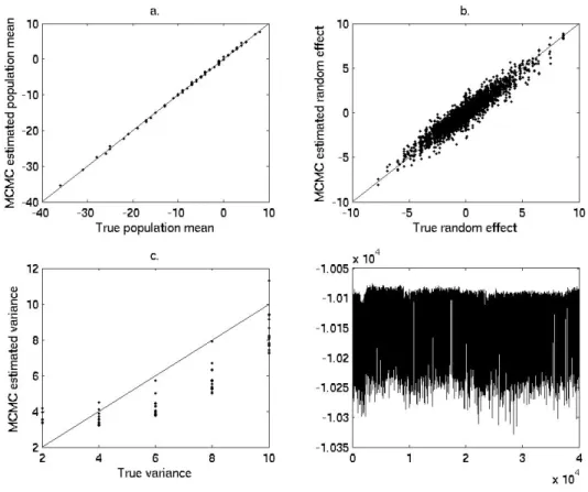
2.2 Plots to evaluate model performance . . . 42
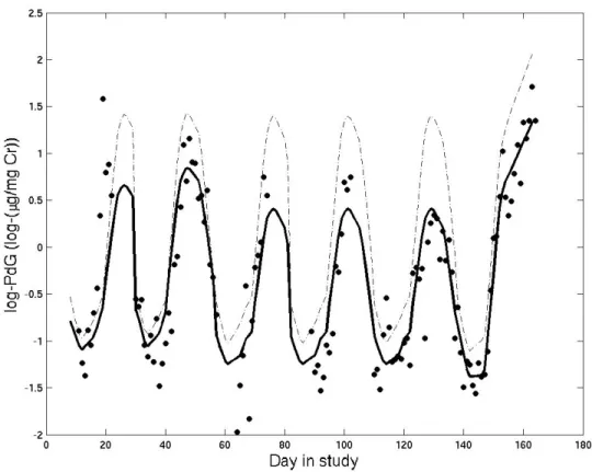
2.3 log(PdG) and estimated regression line for one woman . . . 45
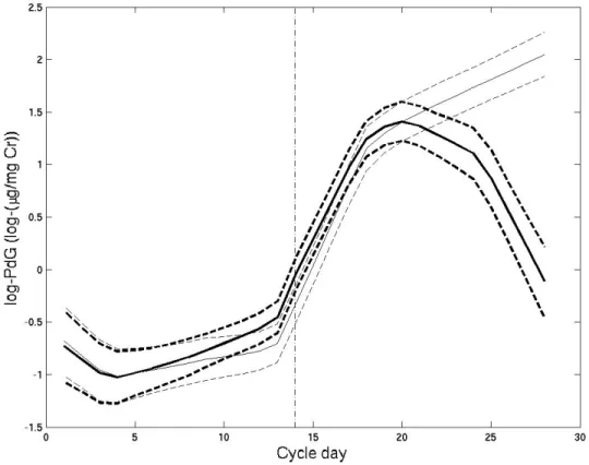
2.4 Estimated log(PdG) trajectories for conception and non-conception cycle 47 2.5 Estimated log(PdG) trajectories for two ovulation days . . . 48
2.6 Unnormalized marginal likelihood and Laplace approximation . . . 49
3.1 Population curves and data for four simulated clusters . . . 72
3.2 Hierarchical class tree for simulated data . . . 74
3.3 Four true simulated clusters and the ten classes identified by the model 75 3.4 Estimated trajectories for final log(PdG) trajectory classes . . . 77
3.5 Data from the final log(PdG) trajectory classes . . . 78
4.1 Population curves, data, and underlying outcome probabilities for four simulated clusters . . . 97
4.2 Mean trajectories and simulated data for the final clusters. . . 98
4.3 Post-ovulatory log(PdG) in early losses . . . 100
4.4 Post-ovulatory log(PdG) in clinical pregnancies . . . 101
4.5 Trajectories and model-estimated probabilities of early loss for the final clusters, first set . . . 102
4.6 Trajectories and model-estimated probabilities of early loss for the final clusters, second set . . . 103
LIST OF TABLES
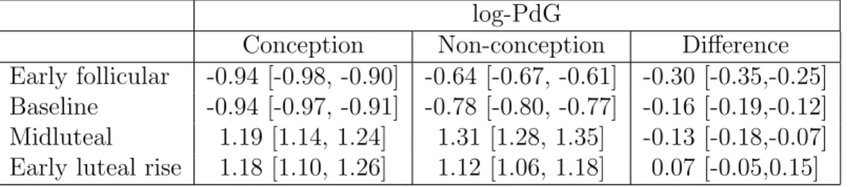
2.1 log(PdG) in conception vs. non-conception cycles . . . 46
2.2 Probability of conception in cycles with very low vs normal/high mid-luteal progesterone . . . 46
CHAPTER 1
LITERATURE REVIEW &
INTRODUCTION
1.1
Motivating Example
1.1.1
Hormones and the menstrual cycle
Certain physiological characteristics, such as hormone levels, basal body temperature,
follicle diameter and cervical mucus are known to vary in accordance with the menstrual
cycle (Stanford et al., 2002). It is of interest to understand how these characteristics
tend to vary within and across different menstrual cycles and in relationship to
predic-tors, such as age or environmental exposures. Also of interest is the inter-relationship
among these different physiological characteristics and their association with fertility
and pregnancy outcomes. In this paper, we develop models appropriate for longitudinal
menstrual data and apply the models to progesterone trajectories. The models can be
generalized to other menstrual and non-menstrual applications based on the concepts
discussed in Section 1.1.3.
A brief review of the menstrual cycle is warranted before discussion of methodology.
bleed and to end the day before the onset of the next menstrual bleed. The first phase of
the cycle, occuring up to the day of ovulation, is termed the follicular phase. Ovulation
marks the transition into the luteal phase, which continues until menstrual bleeding
marks the start of the next cycle (Murphy et al., 1995).
Progesterone levels tend to be low at the cycle start, rise to a peak, and then decrease
Baird et al. (1997). The location of the peak is related to the timing of ovulation within
the cycle. Menstrual cycles tend to vary among and even within women with respect
to cycle length and timing of ovulation. Thus modeling the progesterone trajectory is
not a simple matter of the estimation of a function over a fixed amount of time, with a
fixed ovulation point. Researchers have approached this problem using several different
methods.
Since ovulation is an extremely important reference point in the cycle, marking
the end of the fertile interval and known hormonal changes, many investigators have
chosen simply to restrict consideration to a fixed interval surrounding ovulation, usually
between seven and fourteen days in length (see Baird et al., 1997; Brumback and
Rice, 1998; Massafra et al., 1999 for examples). This allows the incorporation of data
from cycles of various lengths without complicated adjustment for cycle length. Mean
progesterone profiles within the interval can easily be estimated by calculating the mean
progesterone level for each day in the interval, and one can potentially incorporate
covariates and allow for within-woman dependency by using a hierarchical model.
This method has several drawbacks. Truncation yields no information about
pro-gesterone levels on the days outside the chosen interval. In addition, if the interval is
chosen to be too wide it may extend outside the current cycle, and thus reflect
preced-ing or subsequent ovulations. In attempts to model progesterone over the whole cycle,
some investigators have chosen to standardize all cycle lengths to 28 days, effectively
ex-ample). This maintains the relative length of the cycle phases, but masks any inherent
relationship between progesterone and cycle length.
Harlow (1991) point out that, in studies of menstrual cycle diary data, long cycles
tend to be underrepresented, and short cycles tend to be overrepresented. One reason
for this is that long cycles are more likely to be truncated at the start or end of the
study period. If all cycles are standardized to the same length in the analysis, then
the results tend to be more representative of short cycles than of long cycles. Another
source of this disproportionate representation of cycle lengths is that women who tend
to have shorter cycles will contribute more over the study period. This is a problem
of informative cluster size, with each cluster being the set of cycles contributed by a
given woman. In scenarios like this, it is well known that failure to correct for cluster
size can lead to biased inference (Dunson et al., 2003; Romero et al., 1992).
The justification for cycle standardization is entirely based on analytical
conve-nience. That is, there is no evidence to suggest that cycles of different lengths will have
similar characteristics. Studies have shown that menstrual cycle length varies among
women according to BMI, exercise habits, and diet, (Kato et al., 1999) all of which also
affect hormone levels (Unzer et al., 1995; Jasienska et al., 2000). Standardizing the
cycle length obscures the relationship between the length of the menstrual cycle and
the hormone levels.
The relationship between hormone levels and covariates has often been assessed by
creating summary variables (i.e. mean progesterone level during the luteal phase, peak
progesterone level, etc.) and comparing them across levels of the covariate of interest
(see Baird et al., 1997, 1999). The simplicity of this method makes it an attractive
way to model and draw inference about progesterone levels, and differences among
women with respect to summary variables can be biologically informative. However,
the creation of summary variables can mask the richness of the available data and result
in a loss of information.
A recent study by van Zonneveld et al. (2003) compared hormone trajectories
and follicle development in young and older women of reproductive age. To deal with
the differing cycle lengths and ovulation timings, they compared the two groups on
each of three time-scales: days relative to the start of the cycle, days following the
BBT-shift, and days leading up to the luteinizing hormone peak. They concluded that
each time scale provided slightly different information about the hormone trajectory.
this indicates that the understanding of hormones over the menstrual cycle is best
understood through the consideration of multiple reference points.
1.1.2
Early pregnancy study
The data to we use to develop these methods are from the North Carolina Early
Preg-nancy Study (EPS). This prospective cohort study was conducted to determine the risk
of early loss of pregnancy among healthy women. The study population, recruited in
the early 1980s, consisted of 281 couples who were planning to become pregnant. The
women collected daily first-morning urine samples from the time they stopped using
birth control until six months had passed or until the eighth week of clinical pregnancy.
The urine samples were assayed for pregnanediol-3-glucuronide (PdG), a progesterone
metabolite, along with metabolites of many other hormones of interest. Study protocol
and preliminary findings are detailed by Wilcox et al. (1985) and Wilcox et al. (1988),
and the progesterone data are described in Baird et al. (1997).
We restrict attention to the subset of menstrual cycles for which a
hormonally-determined day of ovulation is available. The ovulation day was estimated by the ratio
of estrogen and progesterone metabolites in urine, which decreases abrubtly in response
to ovulation (Wilcox et al., 1998). This measure of ovulation is superior to BBT-based
surge (Ecochard et al., 2001).
In Chapter 2, we examine hormone profiles over the entire menstrual cycle,
com-paring conception and non-conception cycles. In Chapter 3, we consider progesterone
pre-implantation, which we take to be the follicular phase until two days after
ovula-tion. Finally, in Chapter 4, we consider post-ovulatory progesterone in an analysis of
cycles that resulted in a clinical pregnancy and cycles that resulted in an early loss.
1.1.3
Multiple reference point data
Longitudinal data problems can be adapted to a spatial framework through the
iden-tification of multiple reference points in time. van Zonneveld et al. (2003) indicate
that understanding hormones over the menstrual cycle requires the incorporation of
multiple reference points. For simplicity, suppose we consider two reference points: the
start of the cycle, and the day of ovulation. We expect that both of these points will be
informative about progesterone. Each measurement can be given a set of coordinates
(r, s), where r is the cycle day, and s is the day relative to ovulation. If we are correct
in our assumptions about the importance of these reference points in predicting
pro-gesterone, then measurements on days with similar coordinates will tend to be similar,
and our model should reflect this.
Multiple reference points are not unique to menstrual data. They are also important
in epidemiologic studies of exposures. Consider a study with the goal of determining
the relationship between exposure and disease. Subjects in the study provide their date
of exposure and other time-independent covariates of interest. At follow-up visits, the
age of the subject and the disease status are collected. Each measurement can then be
given a set of coordinates (x, y), where xis the number of years since exposure, and y
is the age of the patient at measurement. In this case, the date of exposure and date
of birth are the reference points for a given subject. The investigators may have reason
to believe that time since first exposure, age at first exposure, and current age all play
a role in disease status. All of this information is contained in the coordinate pair for
each measurement and if the investigator is correct, we would expect disease status
measurements with similar coordinates to be similar.
There is a need for innovative methods for multiple reference point data. These
methods should allow the response to vary flexibly in relation to the reference points,
accommodate the estimation and testing of covariate effects, and account for
within-trajectory dependency. In terms of the progesterone data, this model will incorporate
the timing relative to the start of the cycle and the day of ovulation. The model should
be flexible enough to account for the various trajectory shapes that are seen in women,
and to allow for dependency within women and within cycles.
If we choose to think of the model in this spatial framework, then the methods
we develop will have applicability to any problem where the framework applies. This
includes regression settings without reference points and not necessarily longitudinal
as well as true spatial settings, such as image analysis or environmental modeling.
The remainder of this chapter summarizes statistical methods that may be adapted
to the multiple reference point setting. Section 1.2 discusses methods for spatial
model-ing, and Section 1.3 discusses regression methods that may be adapted to the multiple
reference point and spatial settings. Section 1.6 is a summary of preliminary work I
have done to this end. Section 1.7 outlines the dissertation project, which includes the
development of a regression method appropriate for multiple reference point data, a
method for clustering based on the regression coefficients, and a joint model describing
1.2
Methods for spatial modeling
After demonstrating the spatial nature of these data, a natural first step was to explore
methods for spatial analysis. The model we choose should model the data flexibly,
but should also be easily interpretable in a non-spatial manner that is relevant to the
context of the original data problem. In this section, I discuss several methods that
may be adapted to achieve this goal.
1.2.1
Random fields
A random field is a region in space over which random variables may be observed. It may
be finite or infinite, discrete or continuous, and of any dimension. Every observation
from a random field will be associated with a location in space. The interpretation
of random field data depends on these known locations and the spatial correlation
structure of the field. Random fields are most directly seen in true spatial or space-time
data, and are readily applicable to the study of meteorological phenomena (Handcock
and Wallis, 1994), analysis of agricultural field experiments (Allcroft and Glasbey,
2003), image reconstruction (Besag, 1986) and modeling of disease incidence (Waller
et al., 1997; Knorr-Held et al., 2002; Knorr-Held and Richardson, 2003).
Spatial data often has the property that observations that are near each other tend
to be similar. Modeling and inference through the use of a random field is a powerful
way to use this property. The simplest case of this is data smoothing. For example, a
meteorologist may collect air temperature information over a region, then employ an
algorithm to predict the temperature where there were no observations. This is often
accomplished by a technique known as kriging, in which the analyst uses available
data to model the correlation structure as a function of distance between points. The
correlation structure is then used in an iterative procedure to predict the value of
the random field at a large number of unobserved locations given the available data.
(Handcock and Stein, 1993)
A stationary random field has the property that covariance among points is constant
across the field. That is, two points with the same relative position will have the
same correlation regardless of their exact location in the field. The following discussion
assumes that random fields are stationary, although models and computational methods
could be adjusted to relax this assumption.
1.2.2
Markov random fields
Besag (1974) describes a special case of a random field consisting of a finite number of
sites with a univariate random variable observed at each of the sites. For simplicity,
suppose this random field is 1-dimensional with an infinite number of regularly spaced
sites indexed by the integers. Each site r has an associated random variable yr. This
field is called a Markov random field (MRF) if the distribution of yr given y−r, the
observed values at all other sites, depends only upon the values at a finite set of sites
that are ’neighbors’ of r. A simple case is that when the distribution of yr given y−r
depends only upon yr+1 and yr−1. I use ∂r to denote the set of neighbors of site r, and
y(r) to denote the set of observed values at those sites. Neighbor definition is often
arbitrary, and little is known about the impact the chosen neighborhood structure can
have on inference (Assun¸c˜ao et al., 2002).
In this one-dimensional field, distances between locations are fixed. The correlation
between points is only meaningful at specified distances between points, so there is no
need to model correlation as a continuous function of distance. As described in Besag
et al. (1991), the pairwise difference prior can be used to induce this type of correlation
structure. In the context of the one-dimensional random field described above, each
the relative degree of association between site i and j, the pairwise difference prior is:
p(x) ∝ exp
(
−X
i<j
wijφ(yi−yj)
)
(1.1)
where φ is a function that increases with the absolute value of its argument. We wish
to adapt the pairwise difference prior to induce a Markov random field. If we letwij=0
if j /∈∂i, the pairwise difference prior reduces to:
p(x) ∝ exp
(
−X
i∼j
wijφ(yi−yj)
)
(1.2)
where i ∼ j indicates all pairs of i and j such that i < j and i and j are neighbors.
This results in a conditional density where the value of yr depends only on the values
at neighboring sites, and thus we have a Markov random field:
p(xr|x−r) ∝ exp
(
−X
j∈∂i
wijφ(yi−yj)
)
(1.3)
When this conditional distribution is normal, we are working in a Gaussian MRF.
Choosingφ(u) =τ ∗u2/2 in the pairwise difference prior will induce a Gaussian MRF
with the following conditional distribution:
xi|x−i ∼N
P
j∈∂iwijyj
P
j∈∂iwij
, τ−1X
j∈∂i
wij
!
(1.4)
In words, a value at a point given values at all other points depends only on its
neigh-bors, and is normally distributed with the mean corresponding to a weighted average of
the neighbors. This normality is desirable, as many methods are available for sampling
and inference in the Gaussian distribution.
This prior specification illustrates the two ways in which a MRF structure can be
induced. Besag and Kooperberg (1995) call these intrinsic and conditional
autoregres-sions. (The terminology is inconsistent throughout the literature, I will use Besag and
Kooperberg’s distinction). Under intrinsic autoregressive model specification, the joint
prior is specified so that a MRF structure results. This is what we do when we choose
the pairwise difference prior and Markov neighbor structure. Another approach would
have been to specify the prior entirely in terms of a dependent set of conditional
dis-tributions that described a MRF. This method, known as conditional autoregression
or auto-modeling, often leads to an easier computational algorithm. This is not an
issue here, as this special case of the pairwise difference prior (an intrinsic
autoregres-sion) leads to a simple conditional structure. The conditional structure induced by the
special case of the pairwise difference prior above has also been called a Gaussian
con-ditional autoregression (Besag, 1974), or an auto-Gaussian model (Cressie and Chan,
1989). Kaiser and Cressie (2000) discuss the specification of models through conditional
distributions and conditions when and how these conditional distributions correspond
to a joint density. In the specifying of a joint prior, we eliminate the need for this
consideration.
Besag et al. (1991) point out that the pairwise difference prior is improper because
it doesn’t address actual values of random variable across the field, only differences
among the values. However, in the presence of informative data, the resulting posterior
distributions will be proper. If necessary, another way to avoid impropriety would be
to restrict any one of the field values to a plausible finite interval.
This model is easily extended to higher dimensions. On the two-dimensional regular
lattice, each site is indexed by an integer pair (r, s) and has an associated random
variable yrs. This field is a MRF if the distribution of yrs given the observed values at
all other sites depends only upon the values at a finite set of ’neighboring’ sites, ∂rs.
setting, where the the distribution of yrs given the observed values at all other sites
depends only on the values of yr+1,s, yr−1,s, yr,s+1, and yr,s−1. When the field is finite,
this can be simplified to the one-dimensional case by implementing a 1-1 transformation
from the coordinate pairs into the integers, and defining neighbors appropriately. This
can be extended to describe a MRF in n dimensions, although neighbor definition
becomes more complex as the number of dimensions increases.
The adaptability of MRFs to longitudinal data has been demonstrated. Besag
et al. (1995) performed Bayesian logistic regression on longitudinal data, with the
incorporation of unobserved covariates to account for extra-binomial variation. The
data are from a cohort study of prostate cancer deaths, and a spatial model is used
to incorporate both information about age at observation and birth cohort. In other
words, the researchers expected the death rate in 50-year-old men in 1940 to be different
from that of 50-year-old men in 1980, so age alone was not sufficient information. They
found a frequentist logistic regression model with age and cohort to be inadequate (i.e.
there was extra-binomial variation), and chose to use Bayesian methods to account for
this. They treated the data as arising from a binomial MRF, where the coordinates of
the three-dimensional field were age group (i), observation year (j), and cohort number
(k). Note that cohort number is uniquely determined by year and age group. Where
zij is the random unobserved covariate for coordinate (i,j,k) and pij is the probability
of prostate cancer at coordinate (i,j,k), the model was:
ln
pij
1−pij
=µ+θi+φj+ψk+zij (1.5)
In words, the effect of any one of the three coordinates was the same regardless of the
values of the other two. Thus the age effect was the same for all years and cohorts.
A pairwise difference prior was put on θ, φ, and ψ independently, so that each of
these effect was thought to come from a distinct one-dimensional MRF. An alternative
approach would have been to model the log-odds directly, setting up a two-dimensional
neighbor structure with a pairwise-difference prior, under the model:
ln
pij
1−pij
=µij+bk (1.6)
In this model,bkis a cohort random effect with prior mean 0 to allow for the dependence
among observations from the same cohort. This modeling procedure does not separate
the age and year parameters and could allow for a non-linear relationship between the
log-odds, age, and year.
As in the two models above, non-spatial data with multiple reference points in
time (or space) can be adapted to the spatial paradigm for ease of modeling or to
counteract modeling problems. In the current problem, I examine daily measurements
of progesterone levels over the menstrual cycle. Progesterone levels tend to be low at
the start and end of the cycle, with a peak near ovulation. The location of a given
measurement can be classified relative to three reference points: cycle start day, day of
ovulation, and cycle end day.
An important goal of the project is to incorporate covariates that do not vary
systematically with time (i.e. covariates other than the reference points). Assun¸c˜ao
et al. (2002) examine fertility rates across a region of Brazil, fitting a Poisson regression
model for the number of births in each small region. They put a pairwise difference prior
on the model coefficients, allowing the coeffiicients to be more similar in neighboring
regions, but to vary across the entire region. This allows the incorporation of covariate
effects in the usual GLM manner, but gives flexibility in that the covariate effects can
vary across the region. In the multiple reference point problem, these types of covariate
effects would need to be combined with the effects of location relative to the reference
realizations of the Markov random field. Rather, the field is an underlying process, and
the observed data provide information about this process. In the current problem, we
say that the the mean progesterone value at each site is a realization of a MRF. We
observe several observations at each set of coordinates, which will give us information
about the mean (the MRF), but we have no direct observations of the MRF. More
complex HMMs have applications in speech recognition and image analysis (Kunsch
et al., 1995). Given the hierarchical structure of HMMs, Bayesian hierarchical modeling
through MCMC algorithms is well-suited for computation.
The flexibility of the Bayesian hierarchical model is also useful in dealing with other
non-standard features of the progesterone data. Some sites in the region will have no
observations at all, so it is necessary to estimate the mean at these sites through their
correlation with the means at neighboring sites. Additionally, data are not
indepen-dent across the field. Each menstrual cycle contributes multiple data points, and it
is unreasonable to assume that observations within a cycle have the same correlation
structure as observations from different cycles.
The current problem would require a random field over a regular lattice. When
coordinates are not equally spaced, a generalization of the pairwise difference prior can
be employed. Berthelson and Moller (2003) discuss MCMC inference based on this
prior, which takes into account the exact distance between two points in calculating
their degree of association. The MRF neighborhood structure can still apply here, but
careful problem-specific definition is required.
1.3
Regression methods
Rather than thinking of our covariates and times relative to reference points as
coordi-nates in space, and alternative is to think of them as covariates in a regression model.
This works conceptually, as we would expect observations with similar times relative
to reference points to be similar in the same way as a regression model tends to assign
similar response values to observations with similar covariates. This section contains a
review of some flexible regression methods that may be adapted to this setting.
1.3.1
Multivariate linear splines
Holmes and Mallick (2001) developed a semiparametric regression methodology for
modeling a response as a function of a design matrix. The response is modeled using
piecewise linear splines, so that the regression surface consists of hyperplanes across
the covariate space. The number and location of splines are treated as random and
are updated using the reversible jump sampler. The resulting samples are non-smooth
surfaces, but Bayesian model averaging can be applied to the samples to produce a
smooth regression surface.
Bayesian model averaging techniques were developed as a method for dealing with
the uncertainty about model correctness. Often, there is uncertainty about which
model to choose, but the standard response is to pick the ’best’ one and use it for all
inference. Bayesian model averaging allows for the incorporation of model uncertainty
into inference (Raftery et al., 1997). Holmes and Mallick (2001) capitalized on the
properties of Bayesian model averaging to create a smooth regression surface from a
sample of implausible but informative non-smooth surfaces.
Holmes and Mallick (2003) generalized this method to the setting where the outcome
is non-normal and multivariate. It remains, however, to implement this method when
the independent response data are vectors of varying lengths with differing covariate
1.3.2
Non-parametric regression
Lin and Zhang (1999) proposed the generalized additive mixed model (GAMM), where
the linear predictor is the sum of combination of linear functions of the covariates,
non-parametric smooth functions of the covariates, and random effects. These models
allow for flexible covariate effects, but the random effects have an additive effect on the
linear predictor.
Wavelets are orthogonal families of basis functions that can be used to
approxi-mate another function. (Clyde et al., 1998) Modern wavelet theory was brought about
through its applicability to signal and image processing (Akay, 2003) and computer
graphics (Schroder, 1996). Specifically, wavelets are frequently used to remove noise
from signal data and pictures. The ability of wavelets to eliminate noise makes them
broadly applicable in statistical analysis, where the primary goal is to eliminate
ran-dom error and estimate an underlying process. Morris et al. (2003) describe
nonpara-metric wavelet regression in a model with a hierarchical dependence structure, which
was accounted for through random effects. This model shows promise in the current
multiple-reference-point problem, as the dependence structure could be expanded to
allow for spatial association among observations.
Ray and Mallick (2003) propose a wavelet model in the context of a MRF. Their
discussion in framed in the context of image analysis. In summary, they partition
the image and allow the wavelet transformation to vary across partitions. A pairwise
difference prior constrains the transformations to be more similar in neighboring regions
than in non-neighboring regions.
1.3.3
Non-smooth functions
There are times when a function can be expected to have discontinuities in space. In
the context of longitudinal studies, the occurrence of some event (i.e. disease onset,
ovulation) may be known to cause a discontinuity in the outcome of interest. In the
multiple reference point format, if this event was used as a reference point, the model
would need to be flexible enough to allow for a ’jump’ at that reference point. For
example, there is a rapid drop in estrogen levels at ovulation (Alliende, 2003). In
building a spatial model for this quantity, the best model would relax the degree of
association (i.e. reduce the level of smoothing) among neighboring coordinates at points
of discontinuity. This may be a consideration in choosing a modeling strategy for the
multiple-reference point problem.
1.4
Conclusion of initial literature review
The literature review summarizes methods in spatial analysis as well as flexible
re-gression procedures that may be adapted to a spatial framework. These techniques
may be appropriate in the development of methods for multiple reference point data.
Bayesian methods will be used to implement models with broad assumptions on the
spatial structure and covariate effects. Upon preparing the rest of the document,
sev-eral new research questions were encountered. Citations relevant to these questions are
found throughout the ensuing chapters.
1.5
Choosing an approach
Our inital work in building a flexible model for this hormone data focused on the
extension of Markov random field (MRF) theories. The motivation for this type of
model structure was the time-dependence seen in menstrual hormone data, leading
naturally to modeling the correlation between subsequent measurements. After building
a very flexible MRF model for these data, we realized that this approach was limited
MRF approach to an approach using splines, which capture the changes in time as slopes
rather than modeling a point-by-point dependence structure. Section 1.6 outlines the
MRF we applied initially, highlighting some of its successes and limitations. It also
provides some further insight into multiple reference point data and the spatial nature
of regression.
1.6
Preliminary work in MRFs
1.6.1
Data
At the time of preliminary analyses, the EPS data was not yet available so we used
data from Brumback and Rice (1998) to investigate the applicability of Markov random
fields to menstrual data. The data consisted of menstrual cycles truncated to the eight
days preceding through the 15 days following ovulation. To simulate complete cycles
of varied lengths, I added randomly generated numbers of days and corresponding
measurements onto the beginnings and ends of each cycle. Since the cycle lengths were
simulated, these preliminary analyses allow for no inference about cycle length and
progesterone. However, they serve to illustrate how we applied the MRF paradigm to
multiple reference point data.
Daily measurements of progesterone were available, over 69 total cycles. Consider
the set of measurements from one cycle. For each value, we know the day relative to the
start of the cycle (r) and the day relative to ovulation (s). The measurement location
can be defined by the coordinate pair (r, s). Clearly, there are only certain values of
(r, s) that can occur within the natural constraints of the menstrual cycle. Thus I define
the region of interest in the coordinate plane to be the smallest parallelogram-shaped
region that contains all points at which data were observed. The full model specification
is given in Section 1.6.2. In summary, a HMM was fit to the data, incorporating random
effects to account for within-cycle dependence. The model still needs to be expanded to
include covariate effects and to account for multiple cycles contributed from the same
woman.
1.6.2
Model specification
A MRF was used to build a model for the mean log-progesterone level at each
coor-dinate. Let µrs be the unknown mean level at (r, s), and let µ be the n×1 vector
of unknown means. The MRF framework states that, given its neighbors, µrs is
in-dependent of all other elements of µ. We define the neighbors of (r, s) to be the
eight elements that entirely surround the site. Specifically, the neighbors of (r, s) are
(r−1, s), (r+ 1, s), (r, s−1), (r, s+ 1), (r−1, s−1), (r+ 1, s+ 1), (r+ 1, s−1),
and (r−1, s+ 1). For simplicity, this initial model assumes equal unit weights among
all pairs of neighbors. Note that since we are working in a finite lattice, not all sites
will have all eight neighbors. We denote the number of neighbors of (r, s) byprs, and
uv ∼jk is the set of all pairs of neighboring sites. The precision parameter,δ, controls
the degree to which neighboring sites are similar. The desired neighborhood structure
can be induced through the following pairwise difference prior:
p(µ) ∝ δn/2exp
n
− δ 2
X
uv∼jk
(µuv−µ2jk)
o
(1.7)
Letting∂rs be the set of all sites that neighbor (r, s) and µ−(rs) contain all elements of
µexcept for µrs, the corresponding prior conditional structure is:
µrs |µ−(rs)∼N
P
jk∈∂rsµjk
prs
, δ−1prs
!
(1.8)
given µi and the random effects, λi and νi. We also assume that, marginalizing over
the random effects, a measurement at (r, s) is normally distributed with mean µrs. To
illustrate the incorporation of the random effects, suppose (r, s) is inRi, and the
mea-surement at (r, s) from cycle i is calledyi,rs. We then assume the following distribution
of the data:
yi,rs|µrs, λi, νi ∼N λiµrs+νi, τ−1
(1.9)
In this case,λi and νi are the cycle-specific random effects. We assume that, given the
random effects, observations within a cycle are independent. The prior distributions of
λi and νi are normal, centered at 1 and 0 respectively. All elements of λ and ν are a
priori independent.
This specification implies joint normality of all data givenµand the random effects.
Ifyrs is thenrs×1 vector of measurements at (r, s) and λrs and νrs are the
appropri-ately ordered vectors of random effects for all cycles with measurements at (r, s), the
likelihood for the data from site (r, s) is:
π(yrs |µrs,λrs,νrs) = N λrsµrs+νi, τ−1Inrs
(1.10)
The joint data likelihood is normal and can be written as:
π(y|µ,λ,ν, τ) = Y
rs
π(yrs|µrs,λrs,νrs) (1.11)
Since we are not observing direct realizations of the MRF, this is a hidden Markov
model. One attractive effect of this particular specification is that, even though the
MRF structure is present inµ, the data at (r, s), givenµrs are independent of all other
elements of µ. The distributional assumptions are given here.
Likelihood:
π(y|µ,λ,ν, τ)∝
m
Y
i=1
Y
uv∈Ri
τ1/2exp(−τ
2(yi,uv−(λiµuv+νi))
2
) (1.12)
Priors:
π(τ) ∝ τa−1e−bτ
π(δ) ∝ δc−1e−dδ
π(λ) ∝
m
Y
i=1
exp
n
− (λi−1)
2
2σ2
l
o
π(ν) ∝
m Y i=1 exp n − ν 2 i
2σ2
n
o
π(µ) ∝ δn/2exp
n
− δ 2
X
uv∼jk
(µuv−µjk)2)
o
wherea,b, c, d, σl, and σn are specified hyperparameters.
1.6.3
Sampling algorithm
A Gibbs sampling algorithm was implemented to obtain samples from the posterior
dis-tributions. The full conditionals below were used to directly sample from the posterior
distributions ofµ, τ, and δ.
µrs|τ, δ,λ,ν,y ∼ N
δP
jk∼rsµjk +τ(yrs0λrs−τλ0rsνrs)
δprs+τλ0rsλrs
,(δprs+τλ0rsλrs)−1
!
τ|µ, δ,λ,ν,y ∼ Gamma a+ m 2, b+
1 2
X
rs
(yrs−µrsλrs−νrs)0(yrs−µrsλrs−νrs)
!
δ|µ, τ,λ,ν,y ∼ Gamma c+n 2, d+
1 2
X
uv∼jk
(µuv−µjk)2
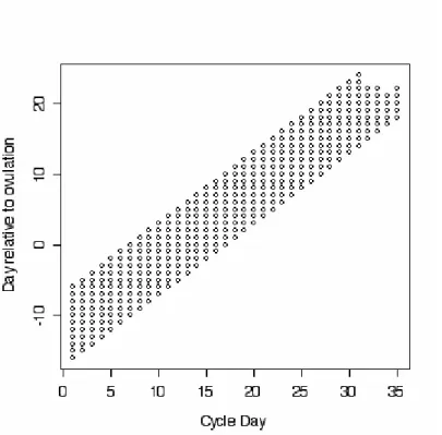
FIGURE 1.1: The region of coordinates covered by the simulated data.
Metropolis steps allowed for sampling from the posterior distributions ofλ andν. The
algorithm was implemented in Matlab. The number of samples collected was 8000,
2000 of which were discarded as burn-in. Convergence was apparent for all parameters,
with slower mixing for the random effect parameters.
1.6.4
Results
The first step was to examine the coordinate region covered by the data. The two
reference points were day relative to cycle start and day relative to ovulation. Figure
1.1 shows the range of coordinates that were defined by the data. The smallest
paral-lelogram containing all these points was the region over which the field was modeled.
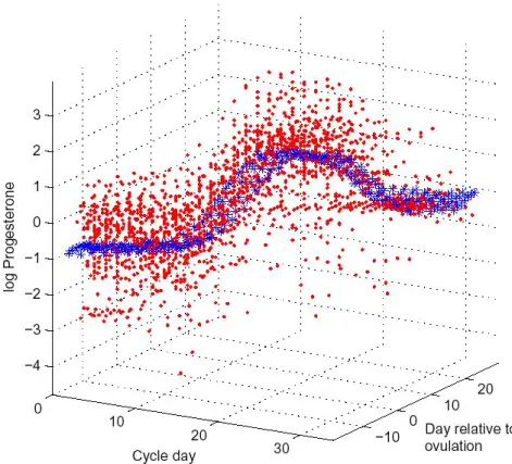
The next step was to determine how the data varied over the region of interest.
FIGURE 1.2: Progesterone over the selected region. Red points are the data, and blue points are the posterior estimate of µ.
Figure 1.2 shows all of the progesterone data, plotted in red according to coordinates.
The posterior estimate of µ is plotted in blue. The versatility of the random effects
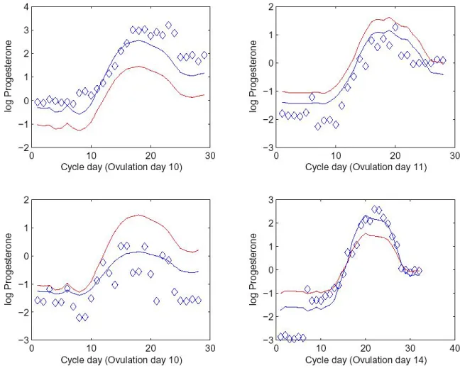
structure is illustrated in Figure 1.3. For four different cycles, these plots illustrate the
data, the mean progesterone according to the coordinates of the cycle days coordinates,
and the estimate of the cycle-specific trajectory, accounting for the random effects.
These show that the random effects structure allows for flexible trajectory shapes.
1.6.5
Discussion of the MRF method
This approach has yielded the desired flexible regression model, but it has several
FIGURE 1.3: Progesterone for four cycles. On each plot, the diamonds are one cycle of data. The red line is the elements ofµ corresponding to that cycle. The blue line is the cycle-specific trajectory, which is the elements ofµadjusted according to the cycle random effects.
informations directly available about slopes, peaks, etc. Posterior information about
these things could be obtained through careful analysis of the samples. Given our
interest in the trajectories as a whole, however, we prefer a method that focuses less
on the point-to-point correlation structure and more on the shape of the curve.
1.7
This Dissertation
To flexibly model the progesterone curves while dealing with some of the issues that
arose in the development of the MRF model, we propose a flexible spline model with
random coefficients. Each of Chapters 2 and 3 is a self-contained article describing
some methodological innovation and demonstrating its application to progesterone
data. Chapter 2 describes a novel nonparametric regression model and demonstrates
its ability to flexibly characterize curves. Chapter 3 outlines a method for introducing a
nonparametric distribution of the coefficients describing the curves and describes a way
to cluster trajectories into groups according to shape. Chapter 4 describes the joint
modeling of curves and outcome variables. Chapter 5 describes some of the implications
CHAPTER 2
BAYESIAN ADAPTIVE
REGRESSION SPLINES FOR
HIERARCHICAL DATA
This chapter considers methodology for hierarchical functional data analysis,
moti-vated by studies of reproductive hormone profiles in the menstrual cycle. Current
methods standardize the cycle lengths and ignore the timing of ovulation within the
cycle, both of which are biologically informative. Methods are needed that avoid
stan-dardization, while flexibly incorporating information on covariates and the timing of
reference events, such as ovulation and onset of menses. In addition, it is necessary to
account for within-woman dependency when data are collected for multiple cycles. We
propose an approach based on a hierarchical generalization of Bayesian multivariate
adaptive regression splines. Our formulation allows for an unknown set of basis
func-tions characterizing the population-averaged and woman-specific trajectories in relation
to covariates. A reversible jump Markov chain Monte Carlo algorithm is developed for
posterior computation. Applying the methods to data from the North Carolina Early
and non-conception cycles.
2.1
Introduction
In many longitudinal studies, each subject contributes a set of data points that can
be considered error-prone realizations of a function of time. Although it is standard
practice to model the longitudinal trajectory relative to a single reference point in time,
such as birth or the start of treatment, there may be several reference points that are
informative about a subject’s response at a given time. One example of reference points
is disease onset, start of treatment, and death in a longitudinal study of quality of life.
The current project uses onset of menses and ovulation as reference points in a study
of reproductive hormones.
Our research was motivated by progesterone data from the North Carolina Early
Pregnancy Study (NCEPS) (Wilcox et al., 1988). Daily measurements of urinary
pregnanediol-3-glucuronide (PdG), a progesterone metabolite, were available for 262
complete menstrual cycles and 199 partial mid-cycle segments from a total of 173
women. It is of special interest to examine the differences in progesterone profiles
be-tween conception and non-conception cycles. The onset of menses marks the start of
the follicular phase of the menstrual cycle, which ends at ovulation. The luteal phase
begins at ovulation and, if no conception occurs, ends at the start of the next menses.
In general, progesterone begins to rise in the follicular phase until several days into the
luteal phase, when it decreases in preparation for the next cycle or, if conception has
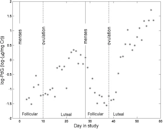
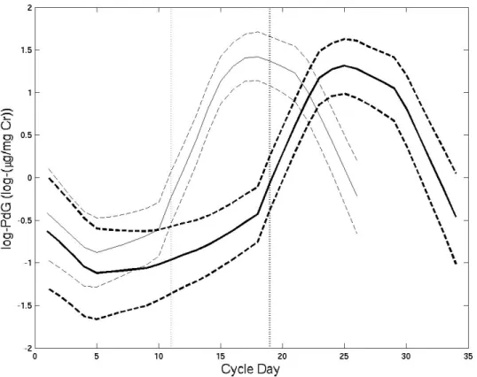
occurred, continues to rise. Figure 2.1 displays log-PdG data from one subject for a
non-conception and subsequent conception cycle.
The most common way to examine hormone data within the menstrual cycle is
FIGURE 2.1: log(PdG) for a non-conception followed by a conception cycle from one subject. Solid lines indicate first day of each cycle, and dashed lines indicate ovulation days.
Brumback and Rice, 1998; Massafra et al., 1999; Dunson et al., 2003 for examples).
This is desirable for ease of modeling, but fails to use all data by discarding days outside
the window. In addition, it ignores cycle length and the relative timing of ovulation
within a cycle. Another approach is to standardize all cycles to a common length.
Zhang et al. (1998) modeled progesterone with smoothing splines after standardizing
cycles to 28 days. Standardization discards biologically important information on the
timing of ovulation, obscuring its well known relationship with hormone trajectories.
van Zonneveld et al. (2003) indicated that both the onset of menses and the day
of ovulation are related to hormone levels within a cycle and implemented separate
analyses for windows around each of these reference points. Ideally, a single model
would allow the response to vary flexibly relative to multiple reference points, while
accommodating covariates and within-woman dependency.
The goal of the analysis is to characterize differences in progesterone profiles
be-tween conception and non-conception cycles. When conception occurs, PdG rises in
response to implantation of the conceptus, which usually occurs around the eighth or
ninth day after ovulation (Baird et al., 1997). We are also interested in differences
before implantation because they may predict the fertility of the cycle. Researchers
have studied conception differences in midluteal (5-6 days after ovulation) and
base-line (preovulatory) PdG. Studies of have shown that conception cycles have elevated
midluteal PdG over paired non-conception cycles with well-timed intercourse or
artifi-cial insemination (Stewart et al., 1993; Baird et al., 1997), but one study (Lipson and
Ellison, 1996) found no difference. None of these three studies found a relationship
between baseline PdG and conception. However, limiting analysis to cycles with
well-timed exposure to semen is biased to include non-conception cycles of inherently low
fertility, failing to represent the true difference between conception and non-conception
low fertility and fails to use all data from women with more or less than two cycles.
In a previous analysis of the NCEPS data which included cycles without well-timed
intercourse, Baird et al. (1999) found that cycles with very low midluteal PdG were
unlikely to be conception cycles. Although midluteal PdG did not monotonically affect
the odds of conception, increased baseline PdG was associated with decreased odds of
conception.
Hormone data are a special case of hierarchical functional data. The daily
mea-surements are subject to assay errors, yielding a noisy realization of the true trajectory
of urinary PdG. The hierarchy results from the multiple cycles contributed by each
woman. Methods for hierarchical functional data typically require that all curves are
observed over or standardized to fall in the same region (Brumback and Rice, 1998;
Morris et al., 2003; Brumback and Lindstrom, 2004). To accommodate the dependence
structure without cycle standardization, we propose a Bayesian method based on a
hierarchical generalization of multivariate adaptive regression splines.
Our approach is related to methods for nonlinear regression and smoothing for
lon-gitudinal and correlated data. Lin and Zhang (1999) proposed the generalized additive
mixed model (GAMM), where the linear predictor is the sum of linear functions of
the covariates, non-parametric smooth functions of the covariates, and random effects.
The GAMM allows for flexible covariate effects, and could potentially be modified to
accommodate reference points. However, they are designed so that random effects vary
linearly with the covariates, which may not be flexible enough to describe the differences
among women in hormone profiles. Fahrmeir et al. (2004) propose a generalization of
the GAMM for space-time data. They model the response using p-splines with a fixed
number of knots, and each covariate enters the model independently. This successfully
accounts for dependence among observations, but further extensions are needed to
al-low for a random number of knots and flexible interactions among covariates. Guo
(2002) introduces a non-parametric flexible model for a population trajectory and the
random effects, but does not allow for the introduction of additional non-parametric
covariate effects.
Motivated by applications to speech data, Brumback and Lindstrom (2004) recently
proposed the use of random time transformations to align times or data features (i.e.
reference points) within subjects. Inference about covariate effects is based on a
com-parison of the estimated transformations. Ratcliffe et al. (2002) give an example of
functional regression using a spline basis, where all the functions are observed over the
same region of time. These methods requires standardization of the time scale as in
Zhang et al. (1998). In addition, Ratcliffe et al. (2002) allows for only one curve per
subject and Brumback and Lindstrom (2004) requires that all subjects contribute a
given number of curves under each covariate condition, both of which are unrealistic in
menstrual studies.
James et al. (2000) describe a method for modeling sparsely-sampled growth curve
data. After choosing a spline basis to represent the curves, they employ reduced rank
principal components analysis to estimate the population mean function. Though their
approach doesn’t require standardization of time, we wish to estimate both the
popu-lation curve and the trajectories themselves.
Holmes and Mallick (2001) proposed Bayesian regression with multivariate linear
splines to flexibly characterize the relationship between covariates and a scalar response
from independent sampling units. The number of knots and their locations are random,
and smooth prediction curves are obtained by averaging over MCMC sampled models.
A extension of this method yielded a generalized nonlinear regression model for a vector
response (Holmes and Mallick, 2003). Our goal is to develop a new hierarchical
adap-tive regression splines approach to accommodate clustered functional data, potentially
compli-cation in longitudinal studies. We incorporate reference point information by including
time relative to each of the reference points as covariates in the regression model.
A popular method for analyzing multivariate response data with spline bases is
seemingly unrelated regression (SUR), in which each subject is allowed a unique set
of basis functions, but the basis coefficients are common to all subjects (Percy, 1992).
We instead use one set of unknown basis functions, allowing the basis coefficients to
vary from subject to subject. To estimate the population regression function, we treat
the subject-specific basis coefficients as random, centered around the population mean
basis coefficients. The resulting model is extremely flexible, and can be used to capture
a wide variety of covariate effects and heterogeneity structures.
In section 2.2, we describe the model, prior structure and a reversible jump Markov
chain Monte Carlo (RJMCMC) (Green, 1995) algorithm for posterior computation. In
section 2.3, we illustrate the performance of the approach for a simulation example.
Section 2.4 applies the method to progesterone data from the NC-EPS, and section 2.5
discusses the results.
2.2
Methods
2.2.1
Prior specification
Typically, the number and locations of knots in a piecewise linear spline are unknown.
By allowing for uncertainty in the knot locations and averaging across the resulting
posterior, one can obtain smoothed regression functions. We follow previous authors
(Green, 1995; Holmes and Mallick, 2001) in using the RJMCMC algorithm to move
among candidate models of varying dimension. Our final predictions are constructed
from averages over all sampled models. We assume a priori that all models are equally
probable, so our prior on the model space is uniform.
Each piecewise linear model,M, is defined by its basis functions (µ1, . . . ,µk), where
µl is p × 1. Consider yij, the jth PdG measurement for subject i. Under model
M, the true relationship between yij and its covariates x0ij = (1, xij2, . . . , xijp) can be
approximated by the piecewise linear model:
yij = k
X
l=1
bil(x0ijµl)++ij, (2.1)
where ij iid
∼ N(0, τ−1). The value of the jth response of subject i is approximated
by a linear combination of the positive portion (denoted by the + subscript) of the
inner products of the basis functions with the covariate vector, xij. We require that
each model contain an intercept basis, so we define (x0ijµ1)+ ≡1 for alli, j. We extend
previous methods by allowing the spline coefficients,bito be subject-specific, assuming
that observations within subject i are conditionally independent givenbi.
Each piecewise linear model is linear in the basis function transformations of the
covariate vectors:
yi =θibi+i, (2.2)
where yi and i are the ni×1 vectors of responses and random errors and bi is the
k×1 vector of subject specific basis coefficients for subjecti. Theni×k design matrix,
θi, contains the basis function transformations of the covariate vectors for subject i:
θi =
1 (x0i1µ2)+ . . . (x0i1µk)+
1 (x0i2µ2)+ . . . (x0i2µk)+
..
. ... ... ...
1 (x0in
iµ2)+ . . . (x
0
iniµk)+
Since we use only the positive portion of each linear spline, it is possible that a
a column of zeros, which is non-informative about the corresponding element of bi).
To address this problem, we standardize each column of the population design matrix,
Θ = (θ10, . . . ,θ0m)0, to have mean 0 and variance 1. Assuming independent subjects, this model specification yields the likelihood:
L(y|b, τ, M)∝
m
Y
i=1
τni2 exp− τ
2(yi−θibi) 0
(yi−θibi)
(2.3)
This likelihood is defined conditionally on the subject-specific basis coefficients, but
we wish to make inferences also on population parameters. Treating the subject-specific
coefficients as random slopes, we specify a Bayesian random effects model where the
subject-specific coefficients are centered around the population coefficients, β. Under
model M of dimension k, the relationship between the population and subject-specific
coefficients is specified through the hierarchical structure:
bi|k ∼Nk(β, τ−1∆−1) ∀i (2.4)
β|k ∼Nk(0, τ−1λ−1Ik)
To avoid over-parameterization of an already flexible model, we assume
indepen-dence among the elements of bi. Thus ∆ = diag(δ), where δ is a k×1 vector. The
elements of δ and the scalars λ and τ are given independent gamma priors:
π(τ, λ,δ)∝τaτ−1exp(−b
ττ)λaλ−1exp(−bλλ) k
Y
l=1
δaδ−1
l exp(−bδδl)
,
where aτ, bτ, aλ, bλ, aδ and bδ are pre-specified hyperparameters. Each of the k−1
non-intercept basis functions contains a non-zero intercept and linear effect for at least
one covariate. Including multiple covariate effects in a single basis allows the covariates
to dependently affect the response (i.e. allows for interactions). The number of non-zero
covariate effects in a particular basis is called the interaction level of the basis.
Under one piecewise linear model, an observation y with covariates x has the
fol-lowing mean and variance:
E(y) =β1+
k
X
l=2
βl(x0µl)+
V(y) = δ−11+
k
X
l=2
δl−1(x0µl)2++τ
−1
The mean and variance can vary flexibly with the covariates and relative to each
other. The elements ofβ can be positive or negative, large or small, and the elements
ofδcan also be large or small. A given basis could contribute substantially to the mean
and negligibly to the variance (i.e. βl and δl are both large), or vice versa, so that the
mean and variance of the response at a given set of covariates are not constrained to
vary together.
2.2.2
Posterior computation
At each iteration, we obtain a piecewise linear model for which the parameters can
be sampled directly from their full conditionals as derived from the priors and the
likelihood following standard algebraic routes. Omitting details, we obtain the following
full conditional posterior distributions:
β|b,δ, λ, τ,D∼Nk
[λIk+m∆]−1∆ m
X
i=1
bi, τ−1[λIk+m∆]−1
bi|β,δ, λ, τ ∼Nki
[θ0iθi+∆]−1[θ0iyi+∆β], τ−1[θ0iθi+∆]−1
i= 1, . . . , m
τ|β,b,δ, λ∼Gammaaτ+
(m+ 1)k+n
bτ + 1 2 m X i=1
[(bi−βi)0∆(bi−βi) + (yi−θibi)0(yi−θibi)] +λβ0β
λ|β,b,δ, τ ∼Gammaaλ+
k
2, bλ+ β0β
2
δl|β,b,δ−l, λ, τ ∼Gamma
aδ+
m
2, bδ+
τ
2
m
X
i=1
(bil−βl)2
l = 0, . . . ,(k−1)
where aGamma(a, b) random variable is parameterized to have expected valuea/band
variance a/b2.
The following is a description of the RJMCMC algorithm we employed:
Step 0: Initialize the model to the intercept-only basis function, where k = 1.
Step 1 : Propose with equal probability either to add, alter or remove a basis function. If k = 1 in the current model, then we cannot remove or change a basis, so we
choose either to add a basis function or to skip to step 2 and redraw the parameters
for the intercept basis.
ADD Generate a new basis function as follows: Draw the interaction level of the basis
uniformly from (1, . . . , p−1) and randomly select the corresponding number of
covariates. Set basis parameters for all other covariates equal to zero. Sample
se-lected basis function parameters fromN(0,1), then normalize to get (µl1, . . . , µlp),
the non-intercept basis parameters. Randomly select one data point,yij, and let
µl0 =x0ij,−1µl,−1. Add the new basis function to the proposed model.
ALTER: Randomly select a basis in the current model. Generate a new basis function
as described above. Replace the selected basis function with the new one
REMOVE: Randomly select a basis in the current model. Delete the selected basis
from the proposed model.
Step 2: Accept the proposed model with appropriate probability (described below).
Step 3: If a proposal to add or remove has been accepted, the dimension of the model has changed. In order to update the parameters from their full conditionals, all
vector parameters must have dimensionk∗ of the new model. It suffices to adjust
the dimension ofβ andδ, as we can then sample {bi}from the full conditionals.
If we’ve added a basis, initialize βk∗, the new element of β, to a pre-determined
initial value and initializeδk∗ to the mean ofδ from the previous model. If a basis
has been removed, delete the corresponding elements of β and δ.
Step 4: Update {bi}, β, τ,δ, and λ from their full conditionals.
Repeat steps 1-4 for a large number of iterations, collecting samples after a burn-in to
allow convergence.
A challenging aspect of the algorithm is comparing models in the RJMCMC sampler.
Our prior assigns equal probability to all piecewise linear models and model proposal is
based on generation of discrete random variables. Under this scenario, the probability,
Q, of accepting a proposed model, M∗, is the Bayes factor comparing it to the current
model, M (Holmes and Mallick, 2003, Denison et al., 2002). The Bayes factor is the
ratio of the marginal likelihoods of the data under the two models:
Q=minh1,p(y|M
∗)
p(y|M)
i
.
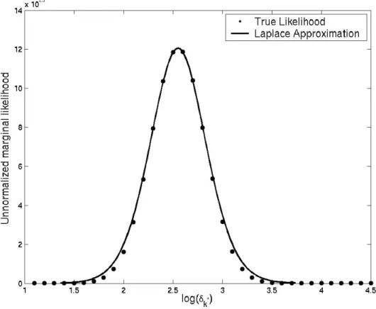
The marginal likelihoods and thus the Bayes factor for this hierarchical model have
no closed form. Consider instead the following marginal likelihood under model M.
p(y|M,δ, λ) =
Z Z Z
L(y|b, τ, λ, M)p(b, τ,β|δ, λ, M)db dβdτ,
that the likelihood can be written:
p(y|M,δ, λ) =C(λ, k)|R|−12(b
τ +
α
2) −(n
2+aτ)
k Y l=1 δ m 2 l m Y i=1
|Ui|
1
2 (2.5)
where
Ui = [∆ +θi0θi]−1
R=λIk+m∆−∆( m
X
i=1
Ui)∆
α=y0y−
m
X
i=1
y0iθiUiθ0iyi−( m
X
i=1
Uiθi0yi)0∆R−1∆( m
X
i=1
Uiθ0iyi)
C(λ, k) = bτ
aτλk
2Γ(n
2 +aτ)
Γ(aτ)(2π)
n
2
In a similar fashion, we can write the marginal likelihood for a proposed modelM∗
of dimension k∗.
p(y|M∗,δ∗, λ∗) =C(λ∗, k∗)|R∗|−12(bτ +α
∗
2 )
−(n2+aτ)
k∗ Y l=1 δ∗ m 2 l m Y i=1
|U∗i|
1
2 (2.6)
Suppose we propose a move from modelM of dimensionkto modelM∗ of dimension
k∗. If we let the acceptance probability be the ratio of the two marginal likelihoods,
then it depends on λ and δ. It also depends on λ∗ and δ∗, for which we do not
have estimates. Since we wish to accept or reject a model based only on its set of
basis functions, we want to minimize the effects of these variance components on the
acceptance probability. Specifically, we assume λ=λ∗ at the current sampled value.
Since δ∗ and δ may be of different dimensions, we cannot assume that they are equal.
Instead, we assume that they are equal in the elements corresponding to bases common
to both models and condition only on those elements.