Vol 5, No 7 (2014)

Available online throug

ISSN 2229 – 5046

ANALYTICAL EXPRESSION OF DENSITY OF A POPULATION IN COMMUNITY ECOLOGY

FROM LOTKA-VOLTERRA MODEL: HOMOTOPY PERTURBATION APPROACH

*

_{V. Ananthaswamy}

a

_{, P. Anusuya}

a

_{, R. Eswaran}

b

_{and L. Rajendran}

a

a

_{Department of Mathematics, The Madura College, Madurai, Tamil Nadu, India.}

b

_{Department of Zoology, The Madura College, Madurai, Tamil Nadu, India.}

(Received On: 11-07-14; Revised & Accepted On: 26-07-14)

ABSTRACT

A

mathematical model of Lotka-Volterra equations, in population ecology is analysed. This model explain the

population density relate to interspecific competitions and carrying capacity. It is devoted to the description of prey– predator or host–parasitoid system dynamics. This paper presents an approximate analytical solution of the general Lotka-Volterra equations. Analytical expressions for density of a species, product concentration and corresponding population density have been derived for all values of parameters using Homotopy perturbation method. The analytical results are compared with our numerical results and are found to be in good agreement.

Keywords: Nonlinear differential equations; Lotka-Volterra equation; Community ecology; Homotopy perturbation method; Numerical simulation.

1. INTRODUCTION

Population models are often used to guide conservation management decisions. Sensitivity analysis of such models can be useful in setting research priorities, by highlighting those parameters that have the most influence on population growth rate. Understanding the processes which drive population growth and dynamics are crucial for conservation managers to make sound ecological decisions for species conservation (Sinclair and Krebs, 2002; Bowden et al., 2003). Many populations may grow to a maximum density which is set by the interplay of resource availability and per capita resource requirements. Resource availability is determined in part by the kind of interactions occurring. All populations are limited in some way. They may be limited intrinsically, by competition for resources within the population, or extrinsically, by a competitor, a predator, a disease, or an abiotic disturbance (Pearl, 1927; Turchin, 1999). Populations of many kinds of organisms, including algae, bacteria, insects, plants, and humans, occasionally escape their limitations and grow to a larger size, sometimes at a fast rate (Delong and Hanson, 2011). Relaxation of both intrinsic and extrinsic regulating factors may stimulate such increases. The nature of interactions among populations (e.g. host plants and herbivores, mutualists, hosts and parasites/parasitoids, predators and prey, competitors) is variable in many ways (for example, Polis, 1984; Bronstein, 1994). Thus, two populations that might normally be mutualists may become a host-parasite system in some circum-stances (Bronstein, 1994).

The Interaction strength–the dynamic consequences of interactions between species–can only be determined by conducting appropriate perturbation experiments, in which certain interactions within communities are ‘isolated’ for further study (Connell, 1983; Mac Nally, 1983; Schoener, 1983). It is crucial to realize that such experiments are the only ways in which to estimate quantities needed to characterize the intensity and nature of the dynamics of interactions (Paine, 1992; Schoener, 1993). Mac Nally (2000) has obtained the mass balance equation in community ecology. In population science research, the Lotka–Volterra model (LVM) is considered a classical dynamic model (Lotka, 1925; Volterra, 1926). The Lotka–Volterra model is one of many continuous (Gertsev and Gertseva, 2004) differential mathematical models devoted to the description of prey–predator or host–parasitoid system dynamics. Lotka-Volterra equations have played a significant role in the development of theoretical ecology, and although there have been many heated debates about whether they are realistic or appropriate for many problems (Goel et al., 1971; Gopalsamy, 1992; Kuang, 1993; Olek, 1994; Ahmad and Lazer, 1995; Zeeman, 1995; Takeuchi, 1996; Ahmad, 1999; Saito, 2001; Zu and Takeuchi, 2012, Capone et al., 2013). It has been broadly used to explain dynamic phenomena in population ecology and other life science fields (Pielou, 1969; Krivan, 1997; Redheffer, 2001; Tonnang et al., 2009). The Lotka-Volterra

Corresponding author:

*

_{V. Ananthaswamy}

a

_,

equations (Pielou, 1969) which describe the population dynamics of prey-predator species have been the subject of several recent papers (Vayenas and Pavlou 2001; Aziz et al., 2012; Shao, 2012; Zu and Takeuchi, 2012; Capone

et al., 2013; Hou, 2012; Hou et al., 2013; Huang et al., 2013). Understanding limiting factors affecting population growth for imperilled species is crucial for conservation and management (Rooney et al., 2004).

A fundamental question in ecology is what determines the density of a population. To our knowledge no rigorous analytical solutions for the density population have been reported. The purpose of this paper is to derive the analytical expressions of Lotka-Volterra model using Homotopy perturbation method for all values of parameters.

2. MATHEMATICAL FORMULATION OF THE PROBLEM

The most commonly used mathematical model for interspecific competition is the classical Lotka–Volterra dynamic equations (Mac Nally, 2000).

(

k

x

y

)

k

x

r

dt

dx

12 1

1

1

−

−

α

=

(1)

(

k

y

x

)

k

y

r

dt

dy

21 2

2

2

−

−

α

=

(2)

where x, y denote the density of population,

r

₁

,

r

₂ represents the growth rate of population in the absence of the competitor,

k

_i is the carrying capacity of the population and

α

is the competition coefficients, which relate the relative competitiveness of a heterospecific competitor to that of a conspecific competitor. The initial conditions are

At

t

=

0

,

x

=

l

(3) At

t

=

0

,

y

=

m

(4)

3. ANALYTICAL SOLUTION OF EQUATION USING HOMOTOPY PERTURBATION METHOD

The Homotopy perturbation method (HPM) was proposed by Ji-Huan He in 1999 (He, 1999, 2000, 2003, 2004a, 2004b, 2005a, 2005b, 2006). In this method, the solution is considered as the summation of an infinite series, which usually converges rapidly to the exact solution. Using the homotopy technique from topology, a homotopy is constructed with an embedding parameter

p

∈

[ ]

0

,

1

which is considered as a “small parameter”. The approximations obtained by the homotopy perturbation method are uniformly valid not only for small parameters, but also for very large parameters. Considerable research has been recently conducted in applying this method to a wide class of linear and nonlinear equations and also to nonlinear oscillator problems, a comparison of the homotopy perturbation method (HPM) and homotopy analysis method (HAM) was made, revealing that the former is more powerful than the latter. Application of the homotopy perturbation method to various integral equations has become a hot topic (Ghorbani and Saberi-Nadjafi, 2008) and references there in).

Recently, many authors have applied the HPM to various problems and demonstrated the efficiency of the HPM for handling non-linear structures and solving various physics and engineering problems. This method is a combination of homotopy in topology and classic perturbation techniques. Ji Huan He used the HPM to solve the Lighthill equation, the Duffing equation and the Blasius equation .The idea has been used to solve non-linear boundary values problems, integral equations and many other problems. The HPM is unique in its applicability, accuracy and efficiently. The HPM uses the imbedding parameter

r

as a small parameter and only a few iterations are needed to search for an asymptotic solution. Using the HPM (see Appendix A), we can obtain the following solution to the eqns. (1)-(4) are as follows:

( )

t

=

x

le

r1t

₊

(

)

(

)

















−

+

−

rt rt

t r

e

r

k

ml

r

e

k

l

e

2

2 1

12 1 1

1 2

1

₁

α

₁

(5)

(

)

(

)



( )

_











−

−

+

=

2 21 2 2

1

k

l

k

m

t

mr

m

t

y

α

₍₈₎

4. RESULTS AND DISCUSSION

The eqns. (5) and (6) represent the most general new approximate analytical expressions for the population

x

and

y

, for the possible values of parameters

r k

_i

,

_i

,

α

_ij. In Fig. 1 analytical expressions of the density of population

x

versus time

( )

t

is plotted for the various values of growth rate of population

(

r

2

=

0

.

8

)

, competition coefficients

(

0

.

01

)

at

the fixed carrying capacity of population (

k

₁

=

10

and

k

₂

=

5

). From this it is inferred that the rate of density of population

x

increases from the initial value of density

(

x

( )

0

=

10

)

. The analytical expressions of the density of population

y

versus time

( )

t

is plotted in Fig.2 for the various values of growth rate of population

(

r

₁

=

0

.

1

)

, competition coefficients

(

α

₁₂

=

0.1,

α

₂₁

=

1

)

at the fixed carrying capacity of population (

k

₁

=

100

and

k

₂

=

50

).

From this it is inferred that the rate of density of population

y

increases from the initial value of density

(

y

( )

0

=

5

)

. From these figures it is inferred that the value of the concentration of population

x

and

y

increases from the initial value of density

x

( )

0

=

l

and

y

( )

0

=

m

respectively when the value of parameters

r

₁and

r

₂increases. The populations of

x

and

y

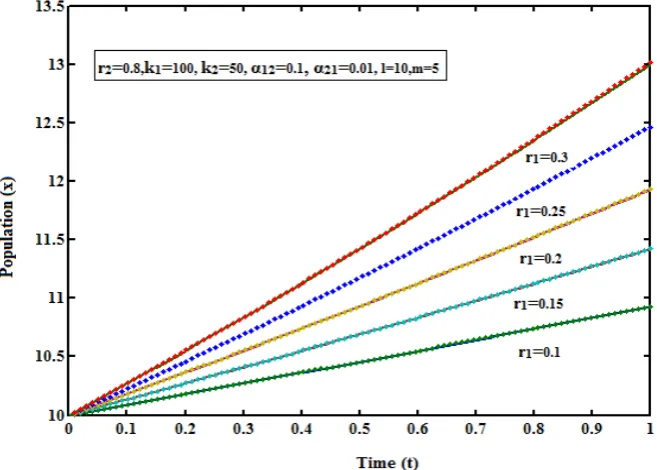
are interdependent and it is one of the many ways of species interaction i.e., Consumer-resource interactions, interactions in which individuals of one species consumes individuals of another species. Examples of consumer-resource interactions include predator-prey interactions and herbivore-plant interactions. These consumer-consumer-resource interactions affect the species involved in different ways, the resource species is negatively impacted while the consumer species is positively impacted.

Fig. - 1: Density of population (x) versus time (t) for various values of r1 and some fixed values of other parameters

(r2 = 0.8, k1=100, k2 = 50, α12=0.1, α21=0.01, l= 10, m=5). The key to the graph: stacked line represents eqn. (5) and

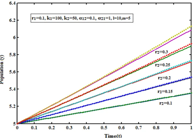
Fig. - 2: Density of population (y) versus time (t) for various values of r2and some fixed values of other parameters

(r1 = 0.1, k1=100, k2 = 50, α12=0.1, α21=1, l= 10, m=5). The key to the graph: tacked line represents eqn. (6) and dotted

line represents the numerical simulation.

5. CONCLUSION

The Lotka-Volterra equations (Pielou, 1969) which describe the population dynamics of prey-predator species are discussed. The approximate analytical solutions to the non-linear reaction equations are derived by using the Homotopy perturbation method. A simple, straight forward and a new method of estimating the density of populations is presented. This solution procedure can be easily extended to all kinds of system of coupled non-linear equation with various complex boundary conditions in population density in community ecology.

ACKNOWLEDGEMENTS

The authors are also thankful to the Secretary Shri. S. Natanagopal, Madura College Board, Madurai, Dr. R. Murali, The Principal and Mr. S. Muthukumar, Head, Department of Mathematics, The Madura College, Madurai, Tamilnadu, India for their constant encouragement.

REFERENCES

1. Ahmad, S. 1999. On the nonautonomous Volterra–Lotka competition equations, Proc. Amer. Math. Soc. 117: 199–204.

2. Ahmad,S. and A.C. Lazer, 1995. On the non autonomous N-competing species problems, Appl. Anal. 57 209–323.

3. Aziz, W. and C. Christopher. 2012. Local integrability and linearizability of three-dimensional Lotka-Volterra systems, Applied Mathematics and Computation. 219 (8): 4067-4081.

4. Bowden, D.C., White, G.C., Franklin, A.B., Ganey, J.L., 2003. Estimating population size with correlated sampling unit estimates. J. Wildlife Manage. 67, 1–10.

5. Bronstein, J.L., 1994. Conditional outcomes in mutualistic interactions. Trends Ecol. Evol. 9, 214–217.

6. Capone, R., S.De Luca and S. Rionero. 2013. On the stability of non-autonomous F perturbed Lotka–Volterra models, Applied Mathematics and Computation, 219 (12): 6868-6881.

12. Gopalsamy, K. 1992. Stability and Oscillations in Delay Differential Equation of Population Dynamics, Kluwer Academic Publishers, Dordrecht, pp. 294–297.

13. He, J.H. 1999. Homotopy perturbation technique, Comp. Meth. Appl. Mech. Engrg. 178 (1999) 257–262. 14. He, J.H. 2000. A coupling method of a homotopy technique and a perturbation technique for non-linear

problems, Internat. J. Non-linear Mech. 35: 37–43.

15. He, J.H. 2003. Homotopy perturbation method: A new non-linear analytical technique, Appl. Math. Comput. 135: 73–79.

16. He, J.H. 2004a. The Homotopy perturbation method for non-linear oscillators with discontinuities, Appl. Math. Comput. 151: 287–292.

17. He, J.H. 2004b. Comparison of homotopy perturbation method and homotopy analysis method, Appl. Math. Comput. 156: 527–539.

18. He, J.H. 2005a. Application of homotopy perturbation method to non-linear wave equations, Chaos Soliton Fractals 26: 695–700.

19. He, J.H. 2005b. Homotopy perturbation method for bifurcation of non-linear problems, Int. J. Non-linear Sci. Numer. Simul. 6: 207–208.

20. He, J.H. 2006. Homotopy perturbation method for solving boundary value problems, Phys. Lett. A 350: 87–88.

21. Hou, Z. 2013. On permanence of Lotka-Volterra systems with delays and variable intrinsic growth rates. Nonlinear Analysis: Real World Applications, 14 (2): 960-975.

22. Hou,Z. 2012 Asymptotic behaviour and bifurcation in competitive Lotka-Volterra Systems, Applied Mathematics Letters, 25 (2):195-199.

23. Huang,Y., Q. Liu, and Y. Liu, 2013. Global asymptotic stability of a general stochastic Lotka†“Volterra system with delays, Applied Mathematics Letter. 26 (1): 175-178.

24. Krivan, V., 1997. Dynamic ideal free distribution: effects of optimal patch choice on predator-prey dynamics. Am. Nat. 149, 164–178.

25. Kuang, Y. 1993. Delay Differential Equations, with Applications in Population Dynamics, Academic Press, NewYork, 1993.

26. Lotka, A.J., 1925. Elements of Physical Biology. Williams & Wilkins, Baltimore, MD.

27. Mac Nally, R.C., 1983. On assessing the significance of interspecific competition to guild structure. Ecology 64, 1646–1652.

28. Mac Nally, R. 2000. Modelling confinement experiments in community ecology: differential mobility among competitors. Ecological Modelling 129 : 65–85

29. Olek, S. 1994. An accurate solution to the multispecies Lotka–Volterra equations, SIAM Rev. 36 (3): 480– 488.

30. Paine, R.T., 1992. Food-web analysis through field measurement of per capita interaction strength. Nature (London) 355, 73–75.

31. Pearl, R., 1927. The growth of populations. Q. Rev. Biol. 2, 532–548.

32. Pielou, E.C. 1969. “An Introduction to Mathematical Ecology,” Wileyybetterscience, New York,

33. Polis, G.A., 1984. Age structure component of niche width and intraspecific resource partitioning: can age groups function as ecological species Am. Nat. 123, 541–564.

34. Redheffer, R.2001. Lotka-Volterra systems with constant interaction coefficients, Nonlinear Anal. 46: 1151-1164.

35. Rooney,T.P., Wiegmann, S.M.,Rogers, D.A., Waller, D.M., 2004. Biotic impoverishment and homogenization in unfragmented forest understory communities. Conserv. Biol. 18, 787–798.

36. Saito, Y. 2001. Permanence and global stability for general Lotka-Volterra predator prey with distributed delays, Nonlinear Anal. 47: 6157-6168.

37. Schoener, T.W., 1983. Field experiments on interspecific competition. Am. Nat. 122, 240–285.

38. Schoener, T.W., 1993. On the relative importance of direct versus indirect effects in ecological communities. In: Kawanabe, H., Cohen, J.E., Iwasaki, K. (Eds.), Mutualism and Community Organization. Behavioural, Theoretical and Food-Web Approaches. Oxford University Press, Oxford, pp. 365–411.

39. Shao, Y. 2012. Globally asymptotical stability and periodicity for a nonautonomous two-species system with diffusion and impulses. Applied Mathematical Modelling. 36(1): 288-300.

40. Sinclair, A.R.E., Krebs, C.J., 2002. Complex numerical responses to top-down and bottom-up processes in vertebrate populations. Philos. Trans. R. Soc. Lond. Ser. B – Biol. Sci. 357, 1221–1231.

41. Sinclair, A.R.E., Krebs, C.J., 2002.Complex numerical responses totop-down and bottom-up processes invertebrate populations.Philos.Trans.R.Soc.Lond.Ser.B–Biol.Sci.357, 1221–1231.

42. Takeuchi, Y. 1996. Global Dynamical Properties of Lotka-Volterra Systems, World Scientific, Singapore. 43. Tonnang, H.E.Z., L.V. Nedorezovb, H. Ochanda, J. Owino and B. Löhr. 2009. Assessing the impact of

biological control of Plutella xylostella through the application of Lotka–Volterra model. ecological modelling220: 60-70.

44. Turchin, P., 1999. Population regulation: a synthetic view. Oikos 84, 153–159.

46. Volterra, V., 1926. Variation and fluctuations of the number of individuals species living together. J. Cons. Perm. Int. Ent. Mer. 3, 3–51 (reprinted in Chapman, R.N., 1993. Animal Ecology, McGraw-Hill, New York). 47. Zeeman, M.L. 1995. Extinction in competitive Lotka–Volterra systems, Proc. Amer. Math. Soc. 123: 87–96. 48. Zu, J. and Y. Takeuchi, 2012. Adaptive evolution of anti-predator ability promotes the diversity of prey

species: Critical function analysis. Biosystems. 109 (2): 192-202.

APPENDIX-A

Basic concept of the He’s Homotopy perturbation method (HPM)

To explain this method, let us consider the following function:

( )

( )

0, r

o

D u

−

f r

=

∈Ω

(A.1) with the boundary conditions of

( ,

)

0, r

o

u

B u

n

∂

=

∈Γ

∂

(A.2)

where

D

_o is a general differential operator,

B

_o is a boundary operator,

f

(

r

)

is a known analytical function and

Γ

is the boundary of the domain

Ω

. In general, the operator

D

_o can be divided into a linear part

L

and a non-linear part

N

. Eq. (A1) can therefore be written as

0

)

(

)

(

)

(

u

+

N

u

−

f

r

=

L

(A.3)

By the Homotopy technique, we construct a Homotopy

v

(

r

,

p

)

:

Ω

×

[

0

,

1

]

→

ℜ

that satisfies

.

0

)]

(

)

(

[

)]

(

)

(

)[

1

(

)

,

(

v

p

=

−

p

L

v

−

L

u

₀

+

p

D

v

−

f

r

=

H

_o (A.4)

.

0

)]

(

)

(

[

)

(

)

(

)

(

)

,

(

v

p

=

L

v

−

L

u

₀

+

pL

u

₀

+

p

N

v

−

f

r

=

H

(A.5)

where p

∈

[0, 1] is an embedding parameter, and

u

₀is an initial approximation of the eqn.(B1) that satisfies the boundary conditions. From the eqns. (A.4) and (A.5) we have

0

)

(

)

(

)

0

,

(

v

=

L

v

−

L

u

0

=

H

(A.6)

0

)

(

)

(

)

1

,

(

v

=

D

v

−

f

r

=

H

o (A.7)

When p=0, the eqns. (A.4) and (A.5) become linear equations. When p =1, they become non-linear equations. The process of changing p from zero to unity is that of

L

(

v

)

−

L

(

u

₀

)

=

0

to

D

_o

(

v

)

−

f

(

r

)

=

0

. We first use the embedding parameter

p

as a “small parameter” and assume that the solutions of the eqns.(A.4) and (A.5) can be written as a power series in

p

:

...

2 2 1

0

+

+

+

=

v

pv

p

v

v

(A.8)

Setting

p

=

1

results in the approximate solution of the eqna. (A.1):

...

lim

_{0 1 2}

1

=

+

+

+

=

→

v

v

v

v

u

p

(A.9)

This is the basic idea of the HPM.

APPENDIX-B

The initial approximations are as follows:

m

y

l

x

₀

(

0

)

=

,

₀

(

0

)

=

(B.3)

...

3

,

2

,

1

for

,

0

)

0

(

,

0

)

0

(

=

y

=

i

=

x

_{i i} (B.4)

The approximate solution of the eqns. (B.1) and (B.2) is

...

2 2 1

0

+

+

+

=

x

px

p

x

x

(B.5)

...

2 2 1

0

+

+

+

=

y

py

p

y

y

(B.6)

Substituting the eqns. (B.5) and (B.6) into the eqns. (B.1) and (B.2) and comparing the coefficients of like powers of p. we obtain the following differential equation

0

0 1 0

0

−

=

x

r

dt

dx

:

p

(B.7)

0

1 0 0 12 1 1 2 0 1 1 1 1

1

−

+

+

=

k

y

x

r

k

x

r

x

r

dt

dx

:

p

α

(B.8)

and

0

0 2 0

0

₋

₌

y

r

dt

dy

:

p

(B.9)

0

2 0 0 21 2 2 2 0 2 1 2 1

1

−

+

+

=

k

y

x

r

k

y

r

y

r

dt

dy

:

p

α

(B.10)

Solving the eqns. (B.7) - (B.10) and using the boundary conditions (B.3) and (B.4) we can obtain the following results:

t r

le

x

1

0

=

(B.11)

(

)

(

)

















−

+

−

=

rt rt rt

e

r

k

ml

r

e

k

l

e

x

2 2 1 12 1 1 1 2 1

1

1

1

α

(B.12) t r

me

y

2

0

=

(B.13)

(

)

(

)

















−

+

−

=

rt rt rt

e

r

k

ml

r

e

k

m

e

y

1 1 2 21 2 2 2 2 2

1

1

1

α

(B.14)

According to HPM we conclude that

( )

lim

(

)

_{0 1}

0

x

t

x

x

t

x

p

=

+

=

→ (B.15)

( )

lim

(

)

_{0 1}

0

y

t

y

y

t

y

p

=

+

=

→ (B.16)

Substituting the eqns. (B.11)-(B.12) into the eqn. (B.15) and (B.13)-(B.14) into the eqn. (B.16) we can obtain the solution in the text.

Source of support: Nil, Conflict of interest: None Declared