DYNAMIC HYDROLOGIC ECONOMIC MODELING OF TRADEOFFS IN HYDROELECTRIC SYSTEMS
Jordan D. Kern
A dissertation submitted to the faculty at the University of North Carolina at Chapel Hill in partial fulfillment of the requirements for the degree of Doctor of Philosophy in the Department of
Environmental Sciences and Engineering in the Gillings School of Global Public Health.
Chapel Hill 2014
Approved by: Gregory Characklis Martin Doyle Jackie MacDonald
iii ABSTRACT
Jordan D. Kern: Dynamic Hydrologic Economic Modeling of Tradeoffs in Hydroelectric Systems (Under the direction of Gregory Characklis)
Hydropower producers face a future beset by unprecedented changes in the electric power industry, including the rapid growth of installed wind power capacity and a vastly increased supply of natural gas due to horizontal hydraulic fracturing (or “fracking”). There is also increased concern surrounding the potential for climate change to impact the magnitude and frequency of droughts. These developments may significantly alter the financial landscape for hydropower producers and have important
ramifications for the environmental impacts of dams.
Incorporating wind energy into electric power systems has the potential to affect price dynamics in electricity markets and, in so doing, alter the short-term financial signals on which dam operators rely to schedule reservoir releases. Chapter 1 of this doctoral dissertation develops an integrated reservoir-power system model for assessing the impact of large scale wind power integration of hydropower resources. Chapter 2 explores how efforts to reduce the carbon footprint of electric power systems by using wind energy to displace fossil fuel-based generation may inadvertently yield further impacts to river
ecosystems by disrupting downstream flow patterns.
Increased concern about the potential for climate change to alter the frequency and magnitude of droughts has led to growing interest in “index insurance” that compensates hydropower producers when values of an environmental variable (or index), such as reservoir inflows, crosses an agreed upon
iv
v
vi
ACKNOWLEDGEMENTS
vii
TABLE OF CONTENTS
LIST OF TABLES ... x
LIST OF FIGURES ... xii
LIST OF ABBREVIATIONS ... xv
INTRODUCTION ... 1
CHAPTER 1: AN INTEGRATED RESERVOIR-POWER SYSTEM MODEL FOR EVALUATING THE IMPACTS OF WIND POWER INTEGRATION ON HYDROPOWER RESOURCES ... 5
1. INTRODUCTION ... 5
2. METHODS ... 7
2.1 Electricity Market Model ... 10
2.2 Reservoir System Model ... 17
3. RESULTS ... 21
3.1 Computing Environment and Solver Algorithm Performance ... 21
3.2 Model Validation ... 23
3.3 Wind Integration Case Study ... 28
4. CONCLUSIONS ... 31
REFERENCES ... 33
CHAPTER 2: THE IMPACTS OF WIND POWER INTEGRATION ON SUB-DAILY VARIATION IN RIVER FLOWS DOWNSTREAM OF HYDROELECTRIC DAMS ... 37
1. INTRODUCTION ... 37
2. METHODS ... 38
2.1 Incorporating Wind Energy in Electric Power Systems ... 38
2.2 Implications for Hydroelectric Dams ... 41
2.3 Modeling Framework ... 42
2.4 Wind Scenarios ... 43
2.5 River Flow Analysis... 44
3. RESULTS ... 45
3.1 Impacts of Wind Energy on Market Prices ... 45
viii
3.3 Impacts of Wind Energy on Richards-Baker Flashiness (RBF) Index ... 53
4. CONCLUSIONS ... 57
REFERENCES ... 59
CHAPTER 3: NATURAL GAS PRICE UNCERTAINTY AND THE SUCCESS OF FINANCIAL HEDGING STRATEGIES FOR HYDROPOWER PRODUCERS ... 62
1. INTRODUCTION ... 62
2. METHODS ... 66
2.1 Modeling Platform and Study Area ... 66
2.2 Study Framework ... 67
2.3 Contract Design... 69
2.4 Contract Premiums ... 75
2.5 Contract Testing ... 77
2.6 Replicating Portfolio ... 79
3. RESULTS ... 81
3.1 Validation of the Reservoir Power System Model ... 81
3.2 Index Basis Risk... 82
3.3 Contract Performance ... 85
3.4 Replicating Portfolio ... 91
4. CONCLUSIONS ... 93
REFERENCES ... 96
CHAPTER 4: THE IMPACTS OF CHANGES IN NATURAL GAS PRICES AND HYDROLOGIC VARIABILITY ON THE COST OF RAMP RATE RESTRICTIONS AT HYDROELECTRIC DAMS ... 98
1. INTRODUCTION ... 98
2. METHODS ... 101
2.1. Modeling Platform and Study Area ... 101
2.2. Study Framework ... 103
3. RESULTS ... 111
3.1. Historical Changes in Cost of Restrictions ... 112
3.2. Cost Model ... 116
3.3. Financial Hedging Strategy ... 118
4. CONCLUSIONS ... 120
REFERENCES ... 122
APPENDIX 1: CHAPTER 1 ... 124
ix
1.1 Plant Costs ... 124
1.2 Simplifying Assumptions ... 127
1.3 Stochastic Real-time Electricity Demand Model ... 128
1.4 Calculation of System Reserve Requirements ... 132
1.5 Unit Commitment Problem ... 134
1.6 Economic Dispatch Problem ... 136
2. Reservoir System Model ... 137
2.1 Hourly Natural Flow Model ... 137
2.2 Hourly Hydropower Dispatch Model... 140
APPENDIX 2: CHAPTER 2 ... 154
APPENDIX 3: CHAPTER 3 ... 156
1. Synthetic Model Inputs ... 156
1.1 Weather Data... 156
1.2 Natural Gas Prices ... 158
1.3 Additional Results ... 163
APPENDIX 4: CHAPTER 4 ... 172
1. Alternative Cost Model ... 172
x
LIST OF TABLES
Table 1. Impacts of wind energy on dam operations and downstream flows...52
Table 2. Strength of correlation (R2 values) between index values and simulated hydropower revenues at Kerr Dam... 83
Table 3. Matrix of Pearson correlation coefficients (R) describing relationship between the seasonal cost of restrictions and fuel prices, peak demand, electricity prices, hydropower production at Roanoke Rapids Dam, and price spread... 114
Table 4. Effect of collar agreement on net seasonal payments paid by downstream stakeholder over the period 2005-2013... 119
Table 5. List of plant specific operating parameters with descriptions and source material...142
Table 6. Reference generation portfolio based on Dominion Zone of PJM (assuming 2010 prices of coal and natural gas of $1.62/MMBtu and $4.86/MMBtu, respectively)...143
Table 7. Calculation of heat rate and fuel cost curves for a 254 MW coal plant with reported eGrid efficiency of 10.27 MMBtu/MWh, assuming a delivered fuel price for coal of $1.62/MMBtu...144
Table 8. Expected heat rate penalties associated with provision of reserves for example 254 MW coal plant with minimum generating capacity of 101.6 MW and a ramp rate of 127MW/h... 145
Table 9. Historical Day-ahead Demand Forecast Error Probabilities...146
Table 10. UC problem time series parameters...147
Table 11. UC problem decision variables...147
Table 12. Unit commitment problem constraints...148
Table 13. ED problem time series parameters...150
Table 14. ED problem decision variables...150
Table 15. Economic dispatch problem constraints...151
Table 16. Time series parameters for hourly hydropower dispatch model...152
Table 17. Decision variables in hourly hydropower dispatch model...152
Table 18. Constraints for hourly hydropower dispatch model...153
xi
Table 20. The 15 wind development scenarios tested in this study...155 Table 21. Contract cost effectiveness measures for contracts i(1)T and i(2)T
for spring coverage period (March, April, May)...163 Table 22. Contract cost effectiveness measures for contracts i(3)T and i(4)T
for spring coverage period (March, April, May)...164 Table 23. Contract cost effectiveness measures for contracts i(1)T and i(2)T
summer season (June, July, August)...165 Table 24. Contract cost effectiveness measures for contracts i(3)T and i(4)T
for summer season (June, July, August)...166 Table 25. Contract cost effectiveness measures for contracts i(1)T and i(2)T
for fall season (September, October, and November)...167 Table 26. Contract cost effectiveness measures for contracts i(3)T and i(4)T
for fall season (September, October and November)...168 Table 27. Contract cost effectiveness measures for contracts i(1)T and i(2)T
for winter season (December, January, February)...169 Table 28. Contract cost effectiveness measures for contracts i(3)T and i(4)T
for winter season (December, January, February)...170 Table 29. Replicating portfolios under average natural gas price volatility...171 Table 30. Model performance and parameters for the cost models calibrated
with historical data from 2005-2013...174 Table 31. Impact of contract duration on mean and standard deviation of net
xii
LIST OF FIGURES
Figure 1. Conceptual framework of integrated reservoir-power system model...9 Figure 2. Three dam cascade in Roanoke River basin...18 Figure 3. Cumulative probability distribution function of relative MIP gap
values for the UC problem from 19 yearlong simulation runs (6935 model solutions),
using a four-minute restriction on solution time by CPLEX...23 Figure 4. Validation of unit commitment problem of electricity market model...25 Figure 5. Comparison of historical and simulated hourly hydropower releases
at Roanoke Rapids Dam...27 Figure 6. Cumulative probability distribution functions of DA (panel A) and real time
(panel B) electricity prices at baseline (0%), 5% and 25% average daily wind market
penetration...29 Figure 7. Impact of wind market penetration on market production (primary y-axis)
and annual profits (secondary y-axis) at Roanoke Rapids Dam...31 Figure 8. Expected changes in mean daily price at different levels of daily wind
market penetration...46 Figure 9. Effect of low-to-moderate forecast wind energy on the day-ahead electricity price... 48 Figure 10. Wind forecast errors as a function of forecast wind energy (panel A)
and probability distribution functions of forecast wind energy for each level of
installed wind power capacity (panel B)...50 Figure 11. Relationship at HIGH installed wind capacity between wind market
penetration (d_WMP), changes in the amount of reserves sold by the Dam ( ),
and changes in the Richards-Baker Flashiness ( ) index...55 Figure 12. Impacts of wind power integration on values of the Richards-Baker
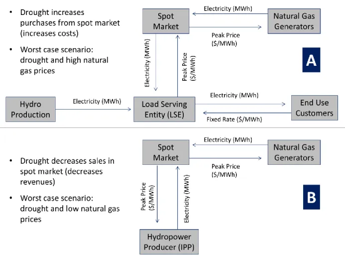
Flashiness (RBF) index...56 Figure 13. Power marketing setup for load serving entity (LSE) with end use customers (A) and
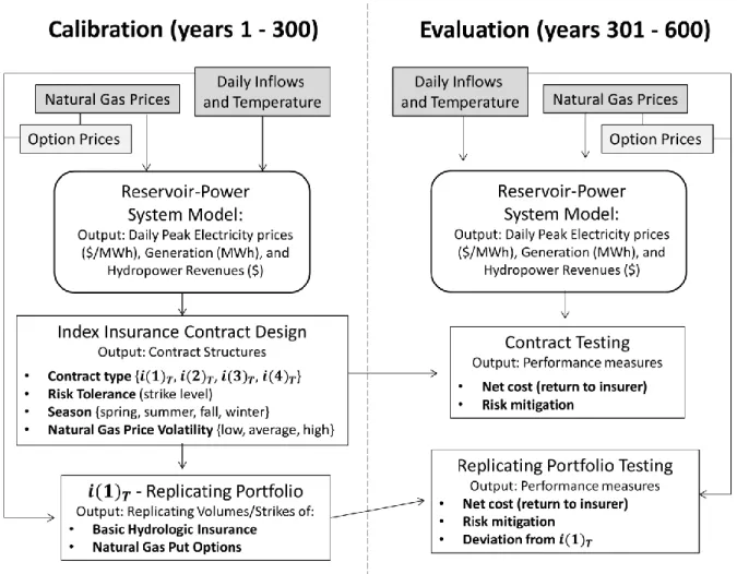
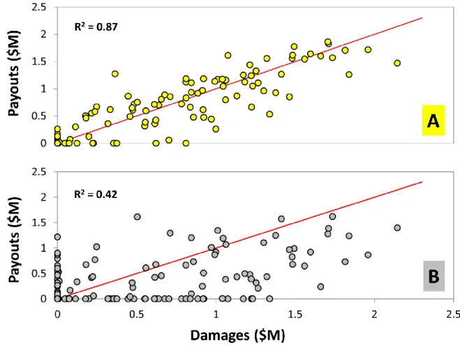
independent power producers (IPPs) (B)...65 Figure 14. Schematic of study framework used in this paper...69 Figure 15. Monthly natural gas prices (1993-2012)...72 Figure 16. Correlation between actual damages experienced by operators of Kerr Dam
(revenues less than $2.7M) and payouts from contracts based on the indices i(1)T
xiii
Figure 17. Increase in premiums and net cost for contracts based on index implemented
for the spring season under low, average, and high natural gas price volatility...87
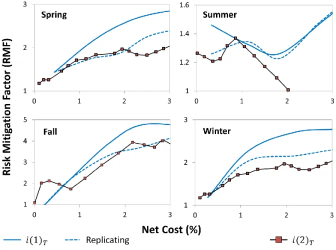
Figure 18. Cost-effectiveness curves for contracts in spring season under average natural gas price volatility...89
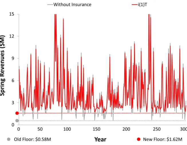
Figure 19. Spring revenues over 300-year testing period without insurance (gray) and with contract based on index (red), assuming a strike of 35% (net cost of 2.6%)...90
Figure 20. Comparison of cost-effectiveness curves for insurance contracts using i(1)T (red lines) and replicating portfolio of hydrological insurance and natural gas put options (black dotted lines)...92
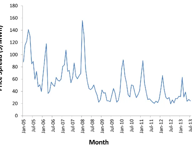
Figure 21. Average monthly price spread in Dominion Zone of PJM Interconnection (2005-2013)...100
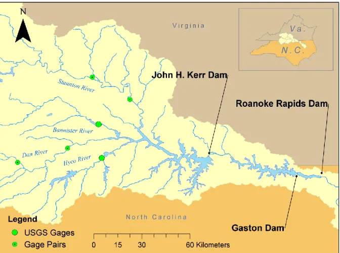
Figure 22. The Lower Roanoke River Basin, featuring John. H. Kerr Dam (US Army Corps of Engineers) and Gaston and Roanoke Rapids dams (Dominion)...102
Figure 23. Experimental setup of paper...104
Figure 24. Non-linear relationship between seasonal generation and the cost of restrictions at a hydroelectric dam, assuming a fixed spread between peak and off-peak electricity prices...107
Figure 25. Schematic of financial risk management strategy for achieving constant conservation payments...110
Figure 26. General decline in seasonal cost of restrictions at Roanoke Rapids Dam and natural gas prices over the period 2005-2013...113
Figure 27. Seasonal cost of restricted operations as a function of total hydropower generation (GWh) and spread between peak and off-peak electricity prices ($/MWh) for the period 2005-2013...116
Figure 28. Model of seasonal cost of restricted operations at Roanoke Rapids Dam as a function of total hydropower generation and price spread...117
Figure 29. Actual and estimated seasonal costs of restricted operations using cost model calibrated with historical hydropower generation and price spread data from 2005-2013...118
Figure 30. Seasonal net payments with and without a collar agreement for the period 2005-2013...120
Figure 31. Standardized heat rate curve for all modeled coal plants...125
Figure 32. Histograms of historical and simulated day-ahead demand forecast error...130
Figure 33. Autocorrelation functions for historical and simulated day-ahead demand forecast error...131
xiv
xv
LIST OF ABBREVIATIONS
CF – capacity factord_WMP – daily average wind market penetration DA – day-ahead
DROM – daily reservoir operations model ED – economic dispatch
EM – electricity market
EPA – US Environmental Protection Agency
EWITS – Eastern Wind Integration and Transmission Study f_WE – forecast wind energy
FERC – Federal Energy Regulatory Commission GW – gigawatt
GWh – gigawatt-hour
IPP – independent power producer LSE – load serving entity
MMBtu –million British thermal units MW – megawatt
MWh – megawatt-hour
NGCC – natural gas combined cycle NGCT – natural gas combustion turbine RBF – Richards-Baker flashiness index RMF – risk mitigation factor
ROR – run of river RT – real-time
1
INTRODUCTION
On an annual basis hydroelectric dams account for a significant fraction (about 7%) of total U.S. electricity generation and roughly two-thirds of the nation’s renewable electricity generation. Although these are important contributions, it is the unmatched operational flexibility and extremely low variable costs of hydroelectric dams that distinguish them as prized assets in electric power systems. Dams can increase electricity output from zero to maximum plant capacity—or decrease it by the same amount—in a matter of minutes. They are also highly efficient (> 90%) at converting potential energy (hydraulic head) to electrical energy, and they entail no fuel costs.
These operating characteristics give hydroelectric dams a tremendous competitive advantage over thermal generation sources (i.e., coal, nuclear, natural gas and oil)—simply put, dams are a cleaner, cheaper and faster way to produce electricity. For more than 75 years, hydroelectric dams have been used by utilities as giant batteries: to store potential energy (reservoir inflows) when electricity demand is low, and produce electricity at maximum rates during high demand periods. This practice decreases system-wide reliance on fossil fuel-based power plants (thereby reducing emissions of CO2 and other pollutants
into the atmosphere) and lowers electricity prices. Hydroelectric dams are also used to provide emergency back-up power during unexpected de-ratings and shut downs at thermal power plants. Thus, they also play a critical role in maintaining system reliability.
2
hydroelectric dams to help meet peak electricity demand in power systems and can cause harmful financial consequences for hydropower producers.
Over the last several decades, research in engineering, hydrology, ecology and economics has contributed to an improved understanding of the tradeoffs that exist between the benefits of hydroelectric dams and their environmental impacts, and has begun to explore the vulnerability of dams (and larger electric power systems) to drought. Through the Federal dam relicensing process—and on occasion, the court system—this research has made headway in establishing management practices at dams that integrate consideration of financial goals, water availability and the protection of river ecosystems.
Nonetheless, hydropower producers face a future beset by unprecedented changes in the electric power industry, including the rapid growth of installed wind power capacity and a vastly increased supply of natural gas due to horizontal hydraulic fracturing (or “fracking”). There is also increased concern surrounding the potential for climate change to impact the magnitude and frequency of droughts. These developments may significantly alter the financial landscape for hydropower producers and have important ramifications for the environmental impacts of dams.
3
portfolios. Chapter 1 of this doctoral dissertation presents a system-based approach for assessing the impact of large scale wind power integration of hydropower resources using an integrated reservoir-power system model. Chapter 2 explores how efforts to reduce the carbon footprint of electric reservoir-power systems by using wind energy to displace fossil fuel-based generation may inadvertently yield further impacts to river ecosystems by disrupting downstream flow patterns. Due to the operational flexibility of hydropower, dams have been suggested as an ideal resource for compensating for both the variability and unpredictability of wind energy. However, coordinated use of wind and hydropower may exacerbate dams’ current impacts on downstream environmental flows, i.e., the magnitude and timing of water flows needed to sustain river ecosystems.
Increased awareness of the vulnerability of hydroelectric dams to drought (along with concern about the potential for climate change to alter the frequency and magnitude of these events) has led to growing interest in risk management strategies that can reduce hydropower producers’ exposure to periods of low reservoir inflows. In recent years, efforts have focused on a risk transfer tool known as “index insurance”, a type of third party contract designed to compensate hydropower producers during droughts. Index insurance is designed to pay-out when values of an environmental variable (or index), such as reservoir inflows, crosses an agreed upon threshold (e.g., low flow conditions). These types of agreements have the potential to dramatically reduce the frequency of very low revenue years for hydropower producers. However, they may also be susceptible to fluctuations in peak electricity prices (i.e., changes in the value of hydropower)—in particular, those caused by price volatility in natural gas markets. Chapter 3 evaluates the need to account for changes in natural gas prices in the design of index-based financial hedging strategies that aim to protect hydropower producers against drought-related damages.
4
the “spread” (difference) between peak and off-peak electricity prices; and 2) total generation at dams (i.e., the availability of water for hydropower production). Variability in these two factors may cause significant seasonal and year-to-year fluctuations in the cost of ramp rate restrictions at dams. This variability may be particularly problematic for downstream stakeholders interested in “purchasing” environmental flow benefits (i.e., compensating a hydropower producer in exchange for the
5
CHAPTER 1:
AN INTEGRATED RESERVOIR-POWER SYSTEM MODEL FOR
EVALUATING THE IMPACTS OF WIND POWER INTEGRATION ON HYDROPOWER
RESOURCES
1. INTRODUCTION
The extent to which large scale integration of wind energy in electric power systems will impact market prices, system costs and reliability may depend greatly on the availability of sources that can quickly change (or ‘ramp’) electricity output [1,2,3]. Due to their capacity for energy storage, low marginal costs, and fast ramp rates, hydroelectric dams are often regarded as an ideal resource for mitigating problematic issues related to wind’s intermittency and unpredictability [4]. In recent years, researchers have investigated a wide range of topics concerning the coordinated use of wind and
hydropower. However, few studies to date have made use of comprehensive reservoir and power system models in assessing the costs and benefits of wind-hydro projects, and the development of such models remains a limiting factor in addressing a number of unanswered questions in this area.
6
increase wind market penetration [12]; and the use of multipurpose dams to integrate wind energy [13]. Pairwise wind-hydro studies, particularly those that include some consideration of a project’s system context, can offer valuable insights. However, they are generally less capable of capturing the more complex, endogenous economic and operational consequences of large scale wind integration for generators and consumers [4].
More comprehensive ‘system-based’ models simulate the effect of wind power integration on the workings of entire electric power systems made up of many different sizes and types of generators. As such, they offer the significant advantage of being able to simulate changes in market prices and system costs that may occur as a result of wind power integration, and then evaluate how these changes could impact the use of hydroelectric dams. However, most previous system-based wind-hydro studies have been conducted by electric power utilities, and detailed modeling information (and even results) from these studies is generally considered proprietary [4]. Examples of system-based studies from academic literature include investigations of the impacts of wind-hydro projects on: the value of wind energy [14]; and the cost of reducing CO2 emissions [15].
7
under a variety of structural, economic, and hydrological conditions, while also maintaining the operational complexity of interconnected reservoir and electric power systems.
At present, there are few systems-based wind-hydro studies available in the scientific literature. This work represents an attempt to begin filling this gap through the development of a systems-based modeling framework for analysis of wind power integration and its impacts on hydropower resources. The model, which relies entirely on publically available information, was developed to assess the effects of wind energy on hydroelectric dams in a power system typical of the Southeastern US (i.e., one in which hydropower makes up < 10% of total system capacity). However, the model can easily reflect different power mixes; it can also be used to simulate reservoir releases at self-scheduled (profit
maximizing) dams or ones operated in coordination with other generators to minimize total system costs. The modeling framework offers flexibility in setting: the level and geographical distribution of installed wind power capacity; reservoir management rules, and static or dynamic fuel prices for power plants. In addition, the model also includes an hourly ‘natural’ flow component designed expressly for the purpose of assessing changes in hourly flow patterns that may occur as a consequence of wind power integration.
2. METHODS
The reservoir-power system model consists of: 1) an electricity market (EM) model; and 2) a reservoir system model. The EM model iteratively solves two linked mixed integer optimization
programs, a unit commitment and economic dispatch problem, to allow a power system operator to meet fluctuating hourly electricity demand. A single iteration of the EM model and its two sub problems yields hourly market prices for a single 24 hour period.
8
Figure 1. Conceptual framework of integrated reservoir-power system model. Orange boxes denote computing order; light grey boxes denote components of the electricity market (EM) model; and dark grey boxes denote components of the reservoir system model.
10 2.1 Electricity Market Model
The EM model was developed in order to simulate the operation of a large power system based on the Dominion Zone of PJM Interconnection (a wholesale electricity market located in the Mid-Atlantic region of the U.S). Dominion’s total generation capacity is approximately 23 gigawatts (GW), with a peak annual electricity demand of roughly 19 GWh. Using the Environmental Protection Agency’s (EPA) 2010 eGrid database, each generator in the utility’s footprint was catalogued by generating capacity (MW), age, fuel type, prime mover and average heat rate (MMBtu/MWh). Specific operating constraints parameters were estimated for each size and type of plant using industry, governmental and academic sources. To reduce the computational complexity of the EM model (i.e., maintain reasonable solution times) units from each plant type were clustered by fixed and variable costs of electricity and reserves, with each cluster of similar generators forming a ‘composite’ plant. The total number of power plants represented in the model was reduced from 68 to a more manageable, yet representative, quantity (24)—with total system wide capacity remaining the same. Each generator in the modeled system belongs to one of eight different power plant types: conventional hydropower, pumped storage hydropower, coal, combined cycle natural gas (NGCC), combustion turbine natural gas (NGCT), oil, nuclear or biomass. Appendix 1
contains detailed operating characteristics of each plant in the modeled generation portfolio.
The EM model has two main components: 1) a unit commitment (UC) problem that represents both ‘day ahead’ electricity and ‘reserves’ markets; and 2) an economic dispatch (ED) problem that represents a 'real time' electricity market [16].
2.1.1 Unit Commitment Problem
11
satisfying system wide requirements for the provision of spinning and non-spinning ‘reserves’
(unscheduled generating capacity that is set aside for the next day as ‘back up’). The objective function of the UC problem is to minimize the cost of meeting forecast electricity demand and reserve requirements over a 96 hour planning horizon, given a diverse generation portfolio:
∑ ∑ (1)
( ) ( ) )
)]
Decision Variables:
indicating spinning reserve provision
= Non spinning reserve capacity scheduled in hour t at generator j (MW)
Parameters
($/MWh)
($)
12
($)
($/MW)
Solution of the UC problem yields a preliminary hourly schedule of DA electricity generation and provision of reserves for each plant in the system over the entire planning horizon (t = 1,2,...96).
However, only the first 24 hours of the calculated operating schedule is considered ‘locked in’— scheduled generation and reserves for later hours, i.e., t = 25, 26,... 96, are immediately discarded. This strategy ensures that plant operating schedules are conditioned on multi-day forecast information for electricity demand, wind availability, and hydropower capacity, but it also makes sure plant operations are formally scheduled no more than 24 hours in advance. Market prices for both DA electricity and reserves for hours t = 1,2,...24 are then determined by the variable cost of the most expensive plant used to meet demand in each market, respectively.
2.1.2 Economic Dispatch Problem
After the UC problem is solved, the model adjusts in real time via the economic dispatch (ED) problem. The ED problem represents the operation of a ‘real time’ (RT) electricity market that compensates for demand forecast error, forced reductions in power plant output, and/or wind forecast errors by scheduling generation from system reserves. The objective function for the EDproblem is to minimize the cost of meeting RT electricity demand over a 24 hour planning horizon (t = 1,2,...24) using generation capacity that was designated one day prior as reserves by the UC problem:
∑ ∑ (2)
13 where,
n = generator in non-spinning reserves portfolio
Decision Variables:
(non-spinning generator)
Parameters:
($/MWh)
($/MWh)
($)
14
Both the UC and ED problems are subject to a number of constraints, which can be separated conceptually into two classes: 1) constraints that enforce adherence to plant specific operating
characteristics (e.g., minimum/maximum generating capacities, maximum ramp rates, minimum up/down times, etc.); and 2) constraints that apply to overall system operation (e.g., the system must always meet hourly demand for electricity and reserves). It is important to note that the EM model does not include consideration of transmission constraints and therefore assumes infinite transmission capacity on all lines. Further details regarding the EM model, including plant specific operating parameters for the modeled generation portfolio, problem constraints, and modeling assumptions, and full mathematical formulations can be found in Appendix 1 section 1.
2.1.3 Wind Development Scenarios
15
make the distance between wind sites and demand centers a more important concern than capacity factor [18].
The wind site selection algorithm yields an assembly of individually modeled wind sites, each of which is associated with two unique time series: 1) a vector of hourly DA wind energy forecasts (MWh); and 2) a vector of hourly wind forecast errors, i.e., actual minus forecast wind energy output (MWh). For a given wind development scenario, time series data are summed across all individually selected sites, yielding a pair of composite wind data vectors—the first describing total DA forecast wind energy across all selected wind sites, and the second describing total wind energy forecast error across the same
collection of wind sites.
2.1.4 Day Ahead and Real Time Electricity Demand
Forecast wind energy is incorporated into the DA electricity market as ‘demand reduction’ by estimating hourly net demand as equal to forecast DA electricity demand (taken from historical databases maintained by PJM Interconnection) [19] minus forecast wind energy (taken from the EWITS database) (Equation 3). RT electricity demand in each hour is simulated stochastically as the sum of three different factors: 1) forced reductions in plant output; 2) demand forecast errors in the DA electricity market; and 3) wind forecast errors:
(3)
+ ∑ , 0) (4)
where,
16 (MWh)
(MW)
The max operator in Equation 4 ensures that RT electricity demand is always greater than or equal to zero, thereby disregarding cases when forecast errors can lead to negative demand. Details regarding the stochastic model used to simulate RT electricity demand are described in section 1.3 of Appendix 1.
2.1.5 Reserve Requirements
Each wind scenario tested assumes a static, baseline reserve requirement consistent with an N minus 1 criterion (i.e., the system operator must always have enough reserves to be able to compensate for the loss of its single largest generator). In addition, each scenario includes an additional dynamic reserve component set as a fixed percentage of forecast wind energy in each hour. The total hourly system reserve requirement for each scenario is then calculated as:
(5)
where,
static N minus 1 reserve requirement (MWh)
17
An approach similar to those described in [20, 21] is used to determine values of . Values of are selected for each scenario such that loss of load probability is equivalent to baseline conditions (i.e., system reliability is equivalent to that of a system with 0% wind market penetration). Detailed discussion of the reserve requirement calculation process, along with typical values of found for different wind levels, can be found in section 1.4 of Appendix 1.
2.2 Reservoir System Model
18
Figure 2. Three dam cascade in Roanoke River basin. USGS gages used to calculate hourly inflows at John H. Kerr reservoir and at the present day site of Roanoke Rapids Dam are shown in green.
2.2.1 Hourly Natural Flow Model
19 2.2.2 Daily Reservoir Operations Model
Reservoir inflows to the furthest upstream dam in the system (John H. Kerr Dam) simulated by the hourly natural flow model are fed directly to a daily reservoir operations model (DROM), which uses time series inputs of inflows, precipitation, and evaporation to drive water balance equations at all three reservoirs. The DROM calculates available storage for hydropower generation at each dam on a daily basis as a function of: reservoir guide curves (schedules of target lake elevation for each day of the calendar year); beginning of period reservoir storage values; hydropower turbine capacities; minimum flow requirements, and water supply contracts. Output from the DROM (in the form of daily volumes of water for release) is then fed to the EM model (for centrally controlled dams) or the hourly hydropower dispatch model (for self-scheduled dams) for more detailed hourly scheduling. For more information on the daily reservoir operations model (data sources, reservoir operating parameters, and model validation), please refer to Kern et al. [23].
2.2.3 Hourly Hydropower Dispatch Model
Any dam assumed to be controlled by a central system operator is scheduled by the EM model, consistent with the objective of minimizing system cost. For self-scheduled dams, however, an hourly hydropower dispatch model is used to maximize profits from the sale of DA electricity, reserves and RT electricity. The hydropower dispatch model works by iteratively solving a deterministic optimization program with the following objective function:
∑
(6)
20 where,
Decision Variables:
ONt = indicating electricity production
STARTt =
Time Series Parameters:
DA_Pt = DA electricity price in hour t ($/MWh) RV_Pt = Reserves price in hour t ($/MWh) RT_Pt = RT electricity price in hour t ($/MWh)
A single iteration of the hydropower dispatch model’s core optimization program yields an hourly schedule of hydropower production in each market (i.e., DA electricity, reserves, and RT electricity) for hours t = 1,2,...96. However, only the first 24 hours of the proposed hydropower schedule are considered ‘locked in’. Sales of electricity and reserves in other hours (t = 25,26,...96) are discarded immediately, and water associated with these discarded sales are retained as available storage. This strategy ensures that reservoir releases are conditioned on expectations of future water availability and market prices, but also makes sure that releases are formally scheduled no more than 24 hours in advance. After the
21
bound to the profits a dam would make in reality by responding to market prices. Further discussion of the hydropower dispatch model for self-scheduled hydroelectric dams (including a complete
mathematical formulation) is presented in section 2.2 of Appendix 1.
3. RESULTS
In the following section, we present results on computational performance and discuss model validation of the reservoir and EM models. In addition, results from three yearlong wind development scenarios are presented in order to demonstrate the capabilities of the integrated modeling framework in evaluating the impact of wind power integration on hydropower resources.
3.1 Computing Environment and Solver Algorithm Performance
The hourly natural flow model and daily reservoir operations model were implemented in Matlab. All optimization problems (the EM and hydropower dispatch models) were formulated using the AMPL language and solved using CPLEX.
By far, the most computationally intensive component of the integrated model is the UC problem of the EM model, due to the large number of binary variables involved in its mathematical structure (three binary variables per generation unit (24), per hour (96), for a total of 6912). As such, efforts to shorten the average simulation time of the larger integrated model focused on limiting the UC model’s role as a performance bottleneck. Solution times for a single iteration of the UC problem—a single iteration simulates hourly prices in the DA electricity and reserves markets for one day—were restricted to four minutes. This time restriction, which ensures that a yearlong modeling run requires roughly 24 hours of computing time (or less), was selected heuristically based on tradeoffs between model detail and solution optimality.
22
objective function values approximate that of the non integer solution. The relative degree of separation between the objective functions of integer and non integer solutions (Equation 7) can be viewed as a measure of solution optimality, and is calculated as:
(7)
where,
23
Figure 3. Cumulative probability distribution function of relative MIP gap values for the UC problem from 19 yearlong simulation runs (6935 model solutions), using a four-minute restriction on solution time by CPLEX. 83% of all individual solutions are within 1% of the optimal non-integer objective function value.
3.2 Model Validation
3.2.1 Electricity Market Model
24
advantage of market power). In panel B of Figure 4, frequency histograms are shown for historical DA electricity prices and ‘corrected’ prices simulated by the UC problem (i.e., simulated prices + $19/MWh). Histograms for both historical and corrected prices are mean centered on $55/MWh, but the distribution of corrected prices shows significantly more kurtosis, due to the smaller number of generating units and corresponding unique prices possible in the EM model. Nonetheless, panels B and C of Figure 4 demonstrate that the UC problem is able to accurately reproduce historical dynamics in DA electricity prices over different timescales.
The UC model also demonstrates a high degree of success in replicating the time series
characteristics and statistical moments of historical reserves prices, which, compared to electricity prices, tend to be significantly much lower and less volatile (typically fluctuating between $5 and $15/MW).
Figure 4. Validation of unit commitment problem of electricity market model. A) cumulative probability distribution functions for simulated and historical mean daily day-ahead electricity prices; B) histogram of corrected (simulated + $19/MWh) and historical mean daily day-ahead
electricity prices; C) daily autocorrelation functions for simulated and historical electricity prices; D) time series of corrected and historical mean day-ahead electricity prices.
26 3.2.2 Reservoir System Model
The hourly natural flow model developed in order to simulate ‘pre-dam’ river flows and current dam sites was able to closely reproduce hourly time series characteristics of natural river flows; however, the model does underestimate total annual inflows to the three dam system by roughly 11%, because it does not account for runoff from floodplains adjacent to the river. A detailed validation of the hourly natural flow model can be found in section 2.1 of Appendix 1. The DROM, which calculates available storage for hydropower generation at each dam on a daily basis, was fully developed as part of a previous study. For details on the DROM (including data sources, reservoir operating parameters, and model validation), please refer to Kern et al. [26].
Output from the DROM (daily volumes of reservoir storage available for hydropower production) is fed to the EM model (for centrally controlled dams) or the hourly hydropower dispatch model (for self-scheduled dams) for hourly scheduling. Figure 5 compares historical hourly reservoir releases at Roanoke Rapids Dam for the year 2006 alongside releases simulated by the EM model (i.e., Roanoke Rapids Dam is assumed to be controlled by the centralized system operator). Panel A of Figure 5 shows a count of simulated and historical hourly flows compartmentalized into four quadrants: i) hours of historical ‘peak’ releases (i.e., reservoir discharges >= 280kL/s) that were correctly simulated as such; ii) hours of
Figure 5. Comparison of historical and simulated hourly hydropower releases at Roanoke Rapids Dam. A) Historical and simulated flows presented in tabular form show the model correctly predicts hourly flows 80% of the time; B) Time-series of historical and simulated reservoir
releases.
28 3.3 Wind Integration Case Study
The EM model was used to simulate market prices for DA and RT electricity and reserves under three different levels (0%, 5% and 25%) of average daily wind market penetration (i.e., wind energy consumed as a fraction of total electricity demand) using land based wind sites located in the Mid-Atlantic region of the US.
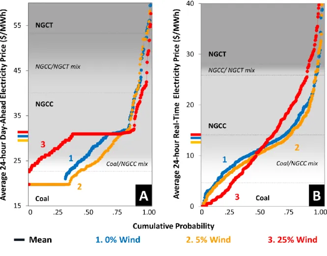
Figure 6 shows CDFs of mean daily prices for DA (panel A) and RT electricity (panel B), estimated from the results of a yearlong simulation that assumed average 2010 fuel prices for coal and natural gas power plants (of about $1.62/MMBtu, and $4.86/MMBtu respectively) [24]. Each panel also indicates the plant type that is dominant in setting the hourly market clearing price for each section of the CDF. Panel A shows that a modest amount (i.e., 5% market penetration) of low cost wind energy reduces the market share of combined cycle natural gas (NGCC) generators in the DA electricity market, which results in less expensive coal generators setting the market clearing price more often. At 25% wind penetration, however, the system relies much more on NGCC generators in order to accommodate lower, more volatile net electricity demand patterns and increased demand for spinning reserves; as a result, NGCC units more frequently set the market clearing price and the bottom 2/3 of the cumulative probability distribution increases in value. At the same time, 25% wind market penetration reduces the frequency of DA price spikes (e.g., especially those caused by periods of peak summer demand)
associated with the use of more expensive oil and combustion turbine natural gas generators. Thus, panel A shows that the upper quartile of the DA price distribution is reduced at 25% wind penetration.
29
Figure 6. Cumulative probability distribution functions of DA (panel A) and real time (panel B) electricity prices at baseline (0%), 5% and 25% average daily wind market penetration. Market clearing plant types are
noted at each price level.
30
the market share of NGCC plants, and annual profits at the dam decrease from $US 8.13 million at baseline to $US 7.81 million at 5% wind penetration.
At 25% wind market penetration, average prices in each market increase due to increased market share of NGCC plants—and profits at the dam increase to $US 9.44 million. More severe negative wind forecast errors entice the dam to significantly increase its sale of reserves and RT electricity on an annual basis, resulting in a sales volume ratio of roughly 1:1 (DA electricity to reserves). This considerable increase in the Dam’s sale of reserves may entail more ‘stop/start’ reservoir releases, which could negatively impact the operational efficiency and longevity of power equipment, and river flows
31
Figure 7. Impact of wind market penetration on market production (primary y-axis) and annual profits (secondary y-axis) at Roanoke Rapids Dam. Results show the dam selling significantly more reserves (and less
DA electricity) at 25% wind market penetration.
4. CONCLUSIONS
32
33
REFERENCES
[1] Lund, H. 2005. Large scale integration of wind power into different energy systems. Energy 30 (13), p. 2402 2412.
[2] U.S. DOE Office of Energy Efficiency and Renewable Energy (EERE). July 2008. 20% Wind Energy
by 2030: Increasing Wind Energy’s Contribution to U.S. Electric Supply. DOE/GO 102008 2567.
Washington: EERE. http://www1.eere.energy. gov/windandhydro/pdfs/41869.pdf.
[3] van Kooten, G.C. 2009. Wind power: the economic impact of intermittency. Lett. Spat. Resour. Sci. 3, 1 17.
[4] International Energy Agency. 2011. “Integration of Wind and Hydropower Systems. Volume 1: Issues, Impacts, and Economics of Wind and Hydropower Integration.”
[5] Belanger, C. and Gagnon, L. “Adding wind energy to hydropower.” Energy Policy 30 (2002) 1279 1284.
[6] Bakos, George. 2002. “Feasibility study of a hybrid wind/hydro power system for low cost electricity production.” Applied Energy. 72, pp. 599 608.
[7] Jaramillo, O. et al. ‘Using hydropower to compliment wind energy: a hybrid system to provide firm power.’ Renewable Energy. 29 (2004) 1887 – 1909.
[8] Bathurst, G.N. and Strbac, G. 2003. “Value of Combining Energy Storage and Wind in Short Term Energy and Balancing Markets. Electric Power Systems Research. Vol. 67, pp. 1 8.
[9] Angarita, J.M. and Usaola, J.G. 2007. “Combining hydro generation and wind energy. Bidding and operation on electricity spot markets.” Electric Power Systems Research. Vol. 77, Issues 5 6, pp. 393 400.
[10] Fernandez, Alisha, Seth Blumsack and Patrick Reed, 2012. “Evaluating Wind Following and Ecosystem Services for Hydroelectric Dams,” Journal of Regulatory Economics 41:1, pp. 139 154. DOI: 10.1007/s11149 011 9177 9.
[11] Castronuovo, E. and Lopes, J.A. ‘On the optimization of the daily operation of a wind-hydro power plant.’ IEEE Transactions on Power Systems, Vol. 19, No. 3, August 2004.
[12] Matevosyan, J. et al. ‘Hydropower planning coordinated with wind power in areas with congestion problems for trading on the spot and the regulating market.’ Electrical Power Systems Research. 79 (2009) 39 48.
[13] Fernandez, Alisha, Blumsack, Seth, and Reed, Patrick. 2013. “Operating constraints and hydrologic variability limit hydropower in supporting wind integration.” Environmental Research Letters. Vol. 8, No. 2.
34
[15] Scorah, H. et al. “The economics of storage, transmission and drought: integrating variable wind power into spatially separated electricity grids.” Energy Economics. 2012. Vol. 34, No. 2. pp. 536-541.
[16] Kirschen, Daniel and Strbac, Goran. Fundamentals of Power System Economics. 2004. Wiley Publishing.
[17] National Renewable Energy Laboratory. “Eastern Wind Integration and Transmission Study.” 2011. [18] Hoppock, D., and Echeverri, D. 2010. “Cost of Wind Energy: Comparing Distant Wind Resources to
Local Resources in the Midwestern United States.” Environmental Science and Technology. Vol. 44(22), pp. 8758 8765.
[19] PJM Interconnection. “ DA Energy Market.” Website. http://www.pjm.com/markets and operations/energy/ DA.aspx. Accessed October 10, 2012.
[20] EnerNex Corporation. “Final Report – 2006 Minnesota Wind Integration Study.” 2006.
[21] Gooi, H.B. et al., “Optimal scheduling of spinning reserve,” IEEE Transactions on Power Systems, vol. 14, no. 4, pp. 1485 1492, November 1999.
[22] Knapp, C. 1976. “The generalized correlation method for estimation of time delay.” IEEE Transactions on Acoustics, Speech and Signal Processing. Volume 24, Issue 4. p. 320 327.
[23] Kern, J. et al. 2011. “Influence of Deregulated Markets on Hydropower Generation and Downstream Flow Regime.” Journal of Water Resources Planning and Management.
[24] Energy Information Administration. Website. http://www.eia.gov. September 2012.
[25] Johnson, R., Oren, S., Svoboda, A. 1997. “Equity and Efficiency of Unit Commitment in Competitive Electricity Markets.” Utilities Policy. Vol. 6, No. 1, p. 9 19.
[26] Lu, B., and Shahidehpour, M. 2005. “Unit Commitment with Flexible Generating units.” IEEE Transactions on Power Systems. Vol. 20, No. 2.
[27] Institute of Electrical and Electronics Engineers (IEEE). “IEEE Reliability Test System.” 1979. IEEE Transactions on Power Apparatus and Systems. Vol. PAS 98, No. 6.
[28] Energy Information Administration. “Updated Capital Cost Estimates for Electricity Generation Plants.” Independent Statistics and Analysis. November 2010.
[29] Peterson, W. L., and Brammer, S. R. 1995. “A Capacity Based Lagrangian Relaxation Unit Commitment with Ramp Rate Constraints.” IEEE Transactions on Power Systems, Vol. 10, No. 2. [30] Kumar, N., Besuner, P., Lefton, S., Agan, D., and Hilleman, D. 2012. “Power Plant Cycling Costs.”
35
[31] Papavasiliou, Anthony, Shmuel S. Oren, Richard P. O'Neill. 2011. “Reserve requirements for wind power integration: A scenario based stochastic programming framework.” IEEE Transactions on Power Systems, Vol. 26, No. 4, p. 2197 2206
[32] North American Electric Reliability Corporation (NERC). “2006 to 2010 Generating Unit Statistical Brochure.” Website. http://www.gadsopensource.com/NERCBroc.aspx. Accessed Oct. 2012
[33] Ortega Vasquez, M., and Kirschen, D. “Optimizing the Spinning Reserve Requirements Using a Cost/Benefit Analysis.” 2007. IEEE Transactions on Power Systems, Vol. 22, No. 1.
[34] North American Electric Reliability Corporation (NERC). “Reliability Concepts.” Website. http://www.nerc.com/files/concepts_v1.0.2.pdf. Accessed Oct. 2012
[35] National Renewable Energy Laboratory. “Operating Reserves and Wind Power Integration: An International Comparison.” 2010.
[36] California Independent System Operator (CAISO). “Spinning Reserve and Non-spinning Reserve.” Website. http://www.caiso.com/docs/2003/09/08/2003090815135425649.pdf
[37] Andracsek, R. “Protecting Your Plant’s Zero to 60”. 2013. Power Engineering Magazine. 117(3). [38] Aggarwal, S., Saini, L., and Kumar, A. “Electricity price forecasting in deregulated markets: A
review and evaluation.” 2009. Electrical Power and Energy Systems. Vol. 31, 13 22.
[39] Bruynooghe, C., Eriksson, A., and Fulli, G. 2010. “Load following operating mode at Nuclear Power Plants (NPPs) and incidence on Operation and Maintenance Costs: Compatibility with Wind Power Variability.” European Commission Joint Research Centre Scientific and Technical Papers. SPNR/POS/10 03 004 Rev. 05
[40] Deane, J.P., Chiodi, A., Gargiulo, M., and O’Gallachoir, B. “Soft linking of a power systems model to an energy systems model.” 2012. Energy. Vol. 42, Issue 1, p. 303 312.
[41] Fenton Jr., F. “Survey of Cyclic Load Capabilities of Fossil Steam Generating Units.” 1982. IEEE Transactions on Power Apparatus and Systems. Vol. PAS 101, No. 6.
[42] Gray, D. 2001. “Correlating Cycle Duty with Cost at Fossil Fuel Power Plants.” Electric Power Research Institute (EPRI) Technical Papers. 1004010.
[43] Lindsay, J., and Dragoon, K. 2010. “Summary Report on Coal Plant Dynamic Performance Capability.” Prepared as part of Renewable Northwest Project.
[44] MIT Energy Initiative. 2010. “Symposium on Managing Large Scale Penetration of Intermittent Renewables.” Website. http://web.mit.edu/mitei/research/reports/intermittent renewables findings.pdf [45] Puga, J.N. 2010. “The Importance of Combined Cycle Generating Plants in Integrating Large Levels
of Wind Power Generation.” The Electricity Journal. Vol. 23, Issue 7.
36
37
CHAPTER 2:
THE IMPACTS OF WIND POWER INTEGRATION ON SUB-DAILY
VARIATION IN RIVER FLOWS DOWNSTREAM OF HYDROELECTRIC DAMS
1. INTRODUCTION
An increased reliance on intermittent wind energy by the electric power industry has augmented the need for sources of generation that can rapidly change power output [1]. Hydroelectric dams can do this more quickly and less expensively than thermal power plants (i.e., coal, natural gas, nuclear, or oil)—as such, they are ideally suited to compensate for the variability and unpredictability of wind energy production. The operational flexibility of dams allows them to start and rapidly increase electricity production when wind is unavailable, and/or curb output when wind is plentiful [2]; and unlike thermal power plants, operating hydroelectric dams in this manner does not entail significant sacrifices in plant efficiency or additional contributions to CO2 emissions [3]. Nonetheless, the coordinated use of wind and
hydropower may exacerbate dams’ current impacts on downstream environmental flows, i.e., the magnitude and timing of water flows needed to sustain river ecosystems.
38
hydroelectric dams on environmental flows in systems with higher levels of intermittent wind power penetrating the market.
Two previous studies have suggested that providing an exclusive “back-up” service to wind farms could compromise a hydroelectric dam’s ability to meet instantaneous minimum flow targets [9,10]; as well as increase the intensity of short-term flow fluctuations [9]. But, these studies give little attention to the larger system context in which wind and hydropower resources operate. As a result, they do not capture the effect wind power integration could have on market prices for electricity and reserves. Market prices, along with reservoir inflows, are often the primary drivers of short-term reservoir release
scheduling. These previous studies also omit consideration of coal and natural gas-fired power plants, which will help bear the brunt of wind power integration in regions with limited hydropower capacity [3]; as well as the level and geographical location of wind energy production, two factors that may be critical in determining how power systems accommodate a significant influx of new wind energy [11].
This study represents an effort to more fully understand the implications of wind power integration for river ecosystems using a system-based approach. An integrated reservoir-power system modeling framework is used to: 1) explore the effects of wind energy on market prices for electricity and reserves in a system with limited (<10%) hydropower capacity under different levels of wind market penetration; and 2) show how shifting financial incentives for hydropower producers could affect reservoir release
schedules and impact sub-daily flow patterns below dams.
2. METHODS
2.1 Incorporating Wind Energy in Electric Power Systems
39
electricity in megawatt-hours (MWh) and an offer price in $/MWh) to provide electricity 24 hours in advance. Bids are collected by a system operator, who uses them to meet forecast electricity demand (schedule generation) for the next day at the lowest possible cost.
In real-time electricity markets, system operators schedule smaller amounts of generation in order to compensate for real-time electricity demand (Equation 1), calculated as the sum of positive day-ahead demand forecast errors (Equation 2), which typically range from 1-3% [15], and forced reductions in power plant output.
(1)
(2)
where, t = hour of the day
EDt = actual electricity demand in hour t (MWh)
f_EDt = day-ahead forecast electricity demand for hour t (MWh)
Outaget = forced reduction in output at power plants in hour t (MWh)
40
quickly. Although rules vary by system, a commonly used requirement is that in any given hour 50% of a system’s supply of reserves should be spinning [3].
Each type of market (i.e., day-ahead electricity, real-time electricity, and reserves) is associated with a separate hourly price generally set by the variable cost of the most expensive resource used to meet demand. Price dynamics in these three markets, which constitute a critical driver of hourly reservoir release schedules at hydroelectric dams, may be significantly affected by large-scale wind integration. Due to the extremely low variable costs of wind energy, forecast wind energy is generally incorporated into day-ahead electricity markets as “demand reduction”; that is, each unit (MWh) of forecast wind energy results in a commensurate reduction in “net” day-ahead electricity demand (Equation 3). Wind energy thus yields lower (but sometimes more volatile) demand patterns for day-ahead electricity.
(3)
where, f_WEt = day-ahead forecast wind energy in hour t (MWh)
The effect of wind energy on demand for real-time electricity depends largely on wind forecasting skill (i.e., the magnitude and sign of wind forecast errors in each hour (Equation 4)), with positive errors serving to reduce real-time electricity demand, and negative errors increasing it (Equation 5).
(4)
(5)
41
Wind power integration also increases demand in reserves markets, with the extent of this increase dependent on the amount of installed wind capacity and the accuracy of wind energy forecasting [16,17]. In this study we employ methods similar to those used in previous studies [3,18,19] to model hourly demand for reserves dynamically as a function of forecast wind energy (Equation 6) using proportionality constants ( calculated based on the level of installed wind power capacity (MW) in the system, as well as the accuracy of wind forecasting at modeled wind sites. For the system presented in this paper, values of range from 4.5% at lower levels of wind capacity up to 29% at higher levels of wind capacity (see Appendix 2 for -values used in this study).
(6)
where,
fixed ‘N minus 1’ reserve requirement (i.e., contingency against loss of largest power plant in the system
value between 0 and 1
2.2 Implications for Hydroelectric Dams
In its simplest form, the problem of maximizing profits at a hydroelectric dam can be viewed as a choice (made in each hour) between: 1) producing day-ahead electricity; and 2) offering reserves and selling real-time electricity. Alternatively, dam operators can choose to do neither and instead retain reservoir storage until a later, more valuable time, since the operational flexibility of dams allow operators to only sell electricity and reserves in hours when they anticipate high prices.
Based on the effects of wind power integration outlined above, we hypothesize that wind energy will decrease prices for day-ahead electricity and increase prices for reserves, and that a profit
42
electricity. In line with this shift in strategy, we also posit that the dam will make more frequent and shorter duration reservoir releases as power production at the dam is increasingly used to compensate for negative wind forecast errors, and that this change in behavior will drive “flashier” river flows
downstream.
2.3 Modeling Framework
An electricity market (EM) model is used to represent the operation of the Dominion Zone of PJM Interconnection, a 23 gigawatt (GW) electric power system in the Mid-Atlantic region of the U.S. The EM model has two main components: a unit commitment problem, which is used to conduct separate hourly markets for day-ahead electricity and reserves, and an economic dispatch problem, which is used to conduct an hourly market for real-time electricity. Each generator in the system belongs to one of eight different power plant types. Listed by fraction of total system capacity, they are: coal (34.4%), natural gas combustion turbine (NGCT) (24.3%), nuclear (15.5%), natural gas combined cycle (NGCC) (13.4%), pumped storage hydropower (6.9%), biomass (1.9%), conventional hydropower (2.1%), and oil (1.5%). The EM model was used to simulate hourly market prices for day-ahead electricity, reserves, and real-time electricity over a 1-year period (2006), under baseline conditions (0MW wind power capacity) and under 15 different wind scenarios (varying the amount and geographical source of installed wind power capacity in the system).
Simulated market prices for each scenario were then sent to a reservoir system model representing the Lower Roanoke River basin (Virginia and North Carolina, U.S.). The reservoir system model uses a deterministic optimization framework along with inputs of market prices to schedule profit-maximizing, hourly reservoir releases at Roanoke Rapids Dam (100MW), subject to operational constraints and water availability. The resultant river flows simulated under baseline conditions and under the 15 wind
43
relevant flow metric, the Richards-Baker Flashiness index [20], to estimate the impacts of wind energy on sub-daily flow patterns.
A complete description of the integrated reservoir-power system model used in this study can be found in [21], which details validation, data sources and full mathematical formulations of the models, as well as plant-specific operating parameters for the modeled generation portfolio, and descriptions of methodologies used to simulate hourly real-time electricity demand and dynamic reserve requirements.
2.4 Wind Scenarios
The 15 wind scenarios explored in this study represent a range of potential development pathways by varying the geographical location and level of installed wind power capacity—two key factors that could determine the impacts of wind energy on market prices [11]. Five different regions in the U.S. are considered: 1) the Southern Plains; 2) the Northern Plains; 3) the Midwest; 4) the Mid-Atlantic; and 5) offshore Atlantic Coast. For each of the five geographical regions, three levels of installed wind power capacity are considered: LOW, MED, and HIGH. These capacity levels correspond to averageannual wind market penetrations (a_WMP) (Equation 8) of 5%, 15%, and 25%, respectively. It is important to note the difference between a_WMP and daily wind market penetration (d_WMP) (Equation 9), which is a dynamic value that fluctuates depending on wind availability and electricity demand.
∑ (8)
∑
(9)
44
Hourly wind data (day-ahead wind energy forecasts and forecast errors) were taken from the updated Eastern Wind Integration and Transmission Study (EWITS) dataset made publicly available by the National Renewable Energy Laboratory [22]. Details regarding contributing U.S. states, total installed wind capacity (GW), and average capacity factors for the 15 wind scenarios can be found in Appendix 2. The algorithm used to select individual wind sites for each scenario is explored in detail in [21].
2.5 River Flow Analysis
The use of flow metrics that describe one or more general characteristics of river flows (i.e., magnitude, duration, frequency, rate-of-change, and timing) is common in efforts to quantify the impact of hydroelectric dams on the downstream environment [23,24,25,26]. In this study, the Richards-Baker flashiness (RBF) index (Equation 10), which has been used in previous efforts to characterize changes in sub-daily flows due to human influences like dams [20,27], is employed to quantify the impacts of wind power integration on downstream flows.
∑ (| | | |)
∑
(10)
where,
45
reversals,” or successive periods of increasing and decreasing flow often produced from dams’ practice of hydropower peaking [29]. It is important to note, however, that while the RBF index is useful for
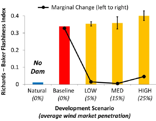
describing changes in hourly flow patterns (some of which may be associated with direct or indirect impacts to riparian ecosystems), results presented in terms of this flow metric cannot be viewed explicitly as measures of ecological damage—only the potential for it to occur. We expect the effects of wind power integration on market prices to incentivize a hydroelectric dam to make more frequent, shorter duration reservoir releases, and anticipate that this change in behavior will lead to higher values of the RBF index.
3. RESULTS
3.1 Impacts of Wind Energy on Market Prices
Figure 8 shows expected changes in mean daily prices, relative to baseline conditions, as a function of daily wind market penetration (d_WMP), using results from all 15 wind scenarios. In general, we find that prices in all three markets move in the same direction in response to increased wind market
46
Figure 8. Expected changes in mean daily price at different levels of daily wind market penetration. Wind energy generally causes prices in all three markets to decrease at daily wind market penetration < 20%.
Above this level, wind energy causes increases in prices.
3.1.1 Day-Ahead Electricity and Reserves
47
plants, which cause them to experience larger losses in efficiency when providing spinning reserves. As a result, the variable cost of spinning reserves from modeled NGCC plants ($7-9/MW) is also higher than that of coal plants ($4-6/MW).
At levels of d_WMP below 20%, forecast wind energy incorporated as “demand reduction” often displaces NGCC plants completely from the day-ahead electricity market (these NGCC plants would otherwise be turned on under baseline conditions). When this happens, the most common result is that less expensive coal plants become the marginal system generator and day-ahead prices decrease. Figure 9 shows a hypothetical example of how forecast wind energy can decrease day-ahead electricity prices by reducing net demand and allowing coal plants to set the market price. In the example shown, 1.5GWh of forecast wind energy reduces net demand by 10%, and the price of day-ahead electricity decreases from $26/MWh (the marginal cost of electricity from a NGCC plant) to $17/MWh (the marginal cost of electricity from a coal plant). Since demand for reserves increases as a function of forecast wind energy (see Equation 6) lower levels of d_WMP result in only modest increases in demand for reserves. If NGCC plants have been displaced from the day-ahead electricity market by wind energy (as shown in Figure 9), the system operator may also have to compensate for the loss of spinning reserves from NGCC plants, because NGCC plants cannot provide spinning reserves if they are offline. But, at lower wind market penetration the system is generally able to meet increased demand for reserves and absorb the loss of NGCC plants using less expensive coal plants and pumped storage. As a result, prices for reserves typically decrease alongside prices for day-ahead electricity.
48
NGCC plants also have higher variable costs than coal plants, increased usage of NGCC plants at high levels of d_WMP often leads to higher prices for reserves and day-ahead electricity.
Figure 9. Effect of low-to-moderate forecast wind energy on the day-ahead electricity price. Figure shows 1.5GWh of forecast wind energy reducing “net” day-ahead electricity demand from 15GWh to 13.5GWh (10%) and the price decreasing from $26/MWh (marginal cost of electricity from a NGCC unit) to $17/MWh
49 3.1.2 Real-Time Electricity
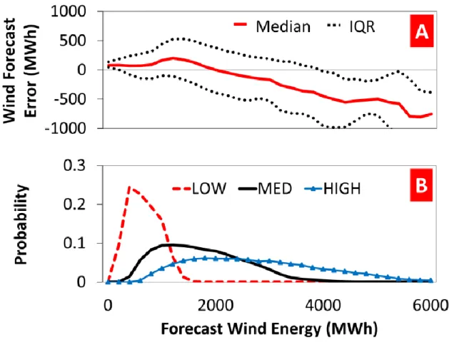
Real-time electricity prices are similarly affected by increases and decreases in the system’s usage of NGCC plants. But the effect of wind energy on real-time electricity prices also depends strongly on the magnitude and sign of wind forecast errors. Panel A of Figure 10 shows the median and interquartile range (IQR) of wind forecast errors as a function of forecast wind energy (f_WE) for all 15 wind
scenarios tested. This graph shows that at high levels of f_WE negative wind forecast errors (increases in real-time electricity demand) are much more likely to occur than positive wind forecast errors (reductions in real-time demand). Figure 10 also shows that the magnitude (absolute value) of negative wind forecast errors generally increases as a function of f_WE.
50
Figure 10. Wind forecast errors as a function of forecast wind energy (panel A) and probability distribution functions of forecast wind energy for each level of installed wind power capacity (panel B). Panel A shows
median and IQR wind forecast errors for the 15 wind scenarios considered. Negative wind forecast errors (increases in real-time electricity demand) are much more likely to occur at HIGH wind capacity.
3.2 Impact of Market Price Changes on Dam Operations
Table 1 shows annual volumes of day-ahead electricity, reserves, and real-time electricity sold by Roanoke Rapids Dam (hereafter ‘the Dam’) at different levels of installed wind power capacity. Data for the wind scenarios (i.e., LOW, MED and HIGH wind capacity) are shown in terms of the average values and standard errors (in italics) for the five geographical regions tested.