Auto Encoding Variational Neural Machine Translation

124

Auto-Encoding Variational Neural Machine Translation

Bryan Eikema & Wilker Aziz

Institute for Logic, Language and Computation University of Amsterdam

[email protected], [email protected]

Abstract

We present a deep generative model of bilin-gual sentence pairs for machine translation. The model generates source and target sen-tences jointly from a shared latent representa-tion and is parameterised by neural networks. We perform efficient training using amortised variational inference and reparameterised gra-dients. Additionally, we discuss the statistical implications of joint modelling and propose an efficient approximation to maximum a pos-teriori decoding for fast test-time predictions. We demonstrate the effectiveness of our model in three machine translation scenarios: in-domain training, mixed-in-domain training, and learning from a mix of gold-standard and syn-thetic data. Our experiments show consistently that our joint formulation outperforms condi-tional modelling (i.e. standard neural machine translation) in all such scenarios.

1 Introduction

Neural machine translation (NMT) systems (Kalchbrenner and Blunsom, 2013; Sutskever et al., 2014; Cho et al., 2014b) require vast amounts of labelled data, i.e. bilingual sentence pairs, to be trained effectively. Oftentimes, the data we use to train these systems are a byproduct of mixing different sources of data. For example, labelled data are sometimes obtained by putting together corpora from different domains ( Sen-nrich et al., 2017). Even for a single domain, parallel data often result from the combination of documents independently translated from dif-ferent languages by difdif-ferent people or agencies, possibly following different guidelines. When resources are scarce, it is not uncommon to mix in some synthetic data, e.g. bilingual data artificially obtained by having a model translate target monolingual data to the source language (Sennrich et al., 2016a). Translation direction,

original language, and quality of translation are some of the many factors that we typically choose not to control for (due to lack of information or simply for convenience).1 All those arguably contribute to making our labelled data a mixture of samples from various data distributions.

Regular NMT systems do not explicitly account for latent factors of variation, instead, given a source sentence, NMT models a single conditional distribution over target sentences as a fully super-vised problem. In this work, we introduce a deep generative model that generates source and target sentences jointly from a shared latent representa-tion. The model has the potential to use the la-tent representation to capture global aspects of the observations, such as some of the latent factors of variation just discussed. The result is a model that accommodates members of a more complex class of marginal distributions. Due to the pres-ence of latent variables, this model requires poste-rior inference, in particular, we employ the frame-work of amortised variational inference (Kingma and Welling,2014). Additionally, we propose an efficient approximation to maximum a posteriori (MAP) decoding for fast test-time predictions.

Contributions We introduce a deep generative model for NMT (§3) and discuss theoretical ad-vantages of joint modelling over conditional mod-elling (§3.1). We also derive an efficient approx-imation to MAP decoding that requires only a single forward pass through the network for pre-diction (§3.3). Finally, we show in §4 that our proposed model improves translation performance in at least three practical scenarios: i) in-domain

1

training on little data, where test data are expected to follow the training data distribution closely; ii) mixed-domain training, where we train a single model but test independently on each domain; and iii) learning from large noisy synthetic data.

2 Neural Machine Translation

In machine translation our observations are pairs of random sequences, a source sentence x = hx1, . . . , xmi and a target sentence y =

hy1, . . . , yni, whose lengthsmandnwe denote by

|x|and|y|, respectively. In NMT, the likelihood of the target given the source

P(y|x, θ) = |y| Y

j=1

Cat(yj|fθ(x, y<j)) (1)

factorises without Markov assumptions (Sutskever et al., 2014; Bahdanau et al., 2015; Cho et al.,

2014a). We have a fixed parameterised function fθ, i.e. a neural network architecture, compute

cat-egorical parameters for varying inputs, namely, the source sentence and target prefix (denotedy<j).

Given a dataset D of i.i.d. observations, the parameters θ of the model are point-estimated to attain a local maximum of the log-likelihood function, L(θ|D) = P

(x,y)∈DlogP(y|x, θ), via

stochastic gradient-based optimisation (Robbins and Monro,1951;Bottou and Cun,2004).

Predictions For a trained model, predictions are performed by searching for the target sentence y that maximises the conditionalP(y|x), or equiva-lently its logarithm, with a greedy algorithm

arg max y

P(y|x, θ)≈greedy y

logP(y|x, θ) (2)

such as beam-search (Sutskever et al.,2014), pos-sibly aided by a manually tuned length penalty. Thisdecision ruleis often referred to as MAP de-coding (Smith,2011).

3 Auto-Encoding Variational NMT

To account for a latent space where global fea-tures of observations can be captured, we intro-duce a random sentence embeddingz ∈ Rd and model the joint distribution over observations as a marginal of p(z, x, y|θ).2 That is,(x, y) ∈ Dis assumed to be sampled from the distribution

P(x, y|θ) = Z

p(z)P(x, y|z, θ)dz . (3)

2_{We use uppercaseP(·) for probability mass functions}

and lowercasep(·)for probability density functions.

where we impose a standard Gaussian prior on the latent variable, i.e. Z ∼ N(0, I), and assume X⊥Y|Z. That is, given a sentence embeddingz, we first generate the source conditioned onz,

P(x|z, θ) = |x| Y

i=1

Cat(xi|gθ(z, x<i)), (4)

then generate the target conditioned onxandz,

P(y|x, z, θ) = |y| Y

j=1

Cat(yj|fθ(z, x, y<j)). (5)

Note that the source sentence is generated with-out Markov assumptions by drawing one word at a time from a categorical distribution parame-terised by a recurrent neural networkgθ. The

get sentence is generated similarly by drawing tar-get words in context from a categorical distribu-tion parameterised by a sequence-to-sequence ar-chitecturefθ. This essentially combines a neural

language model (Mikolov et al.,2010) and a neu-ral translation model (§2), each extended to condi-tion on an addicondi-tional stochastic input, namely,z.

3.1 Statistical considerations

Modelling the conditional directly, as in standard NMT, corresponds to the statistical assumption that thedistributionover source sentences can pro-vide no information about the distribution over target sentences given a source. That is, condi-tional NMT assumes independence ofβ determin-ing P(y|x, β) and α determining P(x|α). Sce-narios where this assumption is unlikely to hold are common: wherexis noisy (e.g. synthetic or crowdsourced), poor qualityxshould be assigned low probabilityP(x|α) which in turn should in-form the conditional. Implications of this assump-tion extend to parameter estimaassump-tion: updates to the conditional are not sensitive to how exoticxis.

Let us be more explicit about how we parame-terise our model by identifying3 sets of param-eters θ = {θemb-x, θLM, θTM}, where θemb-x pa-rameterises an embedding layer for the source lan-guage. The embedding layer is shared between the two model components

P(x, y|z, θ) =

P(x|z, θemb-x, θLM

| {z }

α

)P(y|x, z, θemb-x, θTM

| {z }

β

) (6)

assumption in two ways, namely, by having the two distributions share parameters and by having them depend on a shared latent sentence represen-tation z. Note that while the embedding layer is deterministic and global to all sentence pairs in the training data, the latent representation is stochastic and local to each sentence pair.

Now let us turn to considerations about la-tent variable modelling. Consider a model P(x|θemb-x, θLM)P(y|x, θemb-x, θTM) of the joint distribution over observations that does not em-ploy latent variables. This alternative, which we discuss further in experiments, models each com-ponent directly, whereas our proposed model (3) requires marginalisation of latent embeddings z. Marginalisation turns our directed graphical model into an undirected one inducing further structure in the marginal. See Appendix B, and Figure2in particular, for an extended discussion.

3.2 Parameter estimation

The marginal in Equation (3) is clearly intractable, thus precluding maximum likelihood estimation. Instead, we resort to variational inference ( Jor-dan et al., 1999; Blei et al., 2017) and introduce a variational approximationq(z|x, y, λ)to the in-tractable posteriorp(z|x, y, θ). We let the approx-imate posterior be a diagonal Gaussian

Z|λ, x, y ∼ N(u,diag(ss)) u=µλ(x, y)

s=σλ(x, y)

(7)

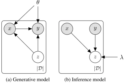
and predict its parameters (i.e. u ∈Rd,s ∈Rd>0) with neural networks whose parameters we denote byλ. This makes the model an instance of a varia-tional auto-encoder (Kingma and Welling,2014). See Figure1in AppendixBfor a graphical depic-tion of the generative and inference models.

We can then jointly estimate the parameters of both models (generative θ and inference λ) by maximising the ELBO (Jordan et al., 1999), a lowerbound on the marginal log-likelihood,

logP(x, y|θ)≥ E(θ, λ|x, y) =

E∼N(0,I)[logP(x, y|z=u+s, θ)] −KL(N(z|u,diag(ss))||N(z|0, I)),

(8)

where we have expressed the expectation with re-spect to a fixed distribution—a reparameterisation available to location-scale families such as the Gaussian (Kingma and Welling, 2014; Rezende

et al., 2014). Due to this reparameterisation, we can compute a Monte Carlo estimate of the gradi-ent of the first term via back-propagation ( Rumel-hart et al., 1986; Schulman et al., 2015). The KLterm, on the other hand, is available in closed form (Kingma and Welling,2014, Appendix B).

3.3 Predictions

In a latent variable model, MAP decoding (9a) re-quires searching forythat maximises the marginal P(y|x, θ) ∝ P(x, y|θ), or equivalently its loga-rithm. In addition to approximating exact search with a greedy algorithm, other approximations are necessary in order to achieve fast predic-tion. First, rather than searching through the true marginal, we search through the evidence lower-bound. Second, we replace the approximate pos-teriorq(z|x, y)by an auxiliary distributionr(z|x). As we are searching through the space of tar-get sentences, not conditioning on y circumvents combinatorial explosion and allows us to drop terms that depend on x alone (9b). Finally, in-stead of approximating the expectation via MC sampling, we condition on the expected latent rep-resentation and search greedily (9c).

arg max y

logP(y|x) (9a)

≈arg max

y Er(z|x)

[logP(y|z, x)] (9b)

≈greedy y

logP(y|Er(z|x)[z], x) (9c)

Together, these approximations enable prediction with a single call to anarg maxsolver, in our case a standard greedy search algorithm, which leads to prediction times that are very close to that of the conditional model. This strategy, and (9b) in par-ticular, suggests that a good auxiliary distribution r(z|x)should approximateq(z|x, y)closely.

We parameterise thisprediction model using a neural network and investigate different options to estimate its parameters. As a first option, we re-strict the approximate posterior to conditioning on xalone, i.e. we approach posterior inference with qλ(z|x) rather than qλ(z|x, y), and thus, we can

user(z|x) =qλ(z|x)for prediction.3 As a second

option, we makerφ(z|x)a diagonal Gaussian and

estimate parametersφto makerφ(z|x)close to the

approximate posteriorqλ(z|x, y) as measured by

3_{Note that this does not stand in contrast to our motivation}

for joint modelling, as we still tie source and target throughz

D(rφ, qλ). For as long asD(rφ, qλ)∈R≥0for ev-ery choice ofφ andλ, we can estimate φjointly withθandλby maximising a modifiedELBO

logP(x, y|θ)≥ E(θ, λ|x, y)−D(rφ, qλ) (10)

which is loosened by the gap betweenrφandqλ.

In experiments we investigate a few options for D(rφ, qλ), all available in closed form for

Gaus-sians, such asKL(rφ||qλ),KL(qλ||rφ), as well as

the Jensen-Shannon (JS) divergence.

Note thatrφis used only for prediction as a

de-codingheuristicand as such need not be stochas-tic. We can, for example, design rφ(x) to be a

point estimate of the posterior mean and optimise

E(θ, λ|x, y)−r_φ(x)−E_q

λ(z|x,y)[z]

2 2 (11)

which remains a lowerbound on log-likelihood.

4 Experiments

We investigate two translation tasks, namely, WMT’s translation of news (Bojar et al.,2016) and IWSLT’s translation of transcripts of TED talks (Cettolo et al.,2014), and concentrate on transla-tions for German (DE) and English (EN) in either direction. In this section we aim to investigate sce-narios where we expect observations to be repre-sentative of various data distributions. As a san-ity check, we start where training conditions can be considered in-domain with respect to test con-ditions. Though note that this does not preclude the potential for appreciable variability in observa-tions as various other latent factors still likely play a role (see§1). We then mix datasets from these two remarkably different translation tasks and in-vestigate whether performance can be improved across tasks with a single model. Finally, we in-vestigate the case where we learn from synthetic data in addition to gold-standard data. For this in-vestigation we derive synthetic data from observa-tions that are close to the domain of the test set in an attempt to avoid further confounders.

Data For bilingual data we use News Commen-tary (NC) v12 (Bojar et al., 2017) and IWSLT 2014 (Cettolo et al.,2014), where we assume NC to be representative of the test domain of the WMT News task. The datasets consist of255,591 train-ing sentences and153,326training sentences re-spectively. In experiments with synthetic data, we subsample 106 sentences from the News Crawl 2016 articles (Bojar et al.,2017) for either German

or English depending on the target language. For the WMT task, we concatenatenewstest2014

andnewstest2015for validation/development (5,172 sentence pairs) and report test results on

newstest2016 (2,999 sentence pairs). For IWSLT, we use the split proposed byRanzato et al.

(2016) who separated6,969training instances for validation/development and reported test results on a concatenation of dev2010, dev2012 and

tst2010-2012(6,750sentence pairs).

Pre-processing We tokenized and truecased all data using standard scripts from the Moses toolkit (Koehn et al., 2007), and removed sen-tences longer than 50tokens. For computational efficiency and to avoid problems with closed vo-cabularies, we segment the data using BPE ( Sen-nrich et al.,2016b) with32,000merge operations independently for each language. For training the truecaser and the BPEs we used a concatenation of all the available bilingual and monolingual data for German and all bilingual data for English.

Systems We develop all of our models on top of Tensorflow NMT (Luong et al.,2017). Our base-line system is a standard implementation of condi-tional NMT (COND) (Bahdanau et al.,2015). To illustrate the importance of latent variable mod-elling, we also include in the comparison a sim-pler attempt at JOINTmodelling where we do not induce a shared latent space. Instead, the model is trained in a fully-supervised manner to maximise what is essentially a combination of two nearly in-dependent objectives,

L(θ|D) = X (x,y)∈D

|x| X

i=1

logP(xi|x<i, θemb-x, θLM)

+ |y| X

j=1

logP(yj|x, y<j, θemb-x, θTM), (12)

namely, a language model and a conditional trans-lation model. Note that the two components of the model share very little, i.e. an embedding layer for the source language. Finally, we aim at investigat-ing the effectiveness of our auto-encodinvestigat-ing varia-tional NMT (AEVNMT).4 AppendixAcontains a detailed description of the architectures that pa-rameterise our systems.5

4

Code available fromgithub.com/Roxot/AEVNMT.

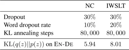
5_{In comparison to C}

NC IWSLT

Dropout 30% 30%

Word dropout rate 10% 20%

KL annealing steps 80,000 80,000

KL(q(z)||p(z))on EN-DE 5.94 8.01

Table 1: Strategies to promote use of latent

representa-tion along with the validarepresenta-tionKLachieved.

Hyperparameters Our recurrent cells are256 -dimensional GRU units (Cho et al., 2014b). We train on batches of64 sentence pairs with Adam (Kingma and Ba, 2015), learning rate3×10−4, for at least T updates. We then perform con-vergence checks every 500 batches and stop af-ter20checks without any improvement measured by BLEU (Papineni et al., 2002). For in-domain training we set T = 140,000, and for mixed-domain training, as well as training with synthetic data, we setT = 280,000. For decoding we use a beam width of 10 and a length penalty of 1.0. We investigate the use of dropout (Srivastava et al.,

2014) for the conditional baseline with rates from 10% to 60% in increments of 10%. Best valida-tion performance on WMT required a rate of 40% for EN-DEand 50% for DE-EN, while on IWSLT it required50%for either translation direction. To spare resources, we also use these rates for train-ing the simple JOINTmodel.

Avoiding collapsing to prior Many have no-ticed that VAEs whose observation models are pa-rameterised by strong generators, such as recur-rent neural networks, learn to ignore the latent rep-resentation (Bowman et al., 2016;Higgins et al.,

2017;Sønderby et al.,2016;Alemi et al.,2018). In such cases, the approximate posterior “collapses” to the prior, and where one has a fixed prior, such as our standard Gaussian, this means that the pos-terior becomes independent of the data, which is obviously not desirable. Bowman et al. (2016) proposed two techniques to counter this effect, namely, “KLannealing”, and target word dropout. KL annealing consists in incorporating the KL term of Equation (8) into the objective gradually, thus allowing the posterior to move away from the prior more freely at early stages of training. After

and possibly a prediction network. However, this does not add much sequential computation: the inference network can run in parallel with the source encoder, and the source lan-guage model runs in parallel with the target decoder.

Objective BLEU↑

ELBOx,y−KL(rφ(z|x)||qλ(z|x, y)) 14.7 ELBOx,y−KL(qλ(z|x, y)||rφ(z|x)) 14.8 ELBOx,y−JS(rφ(z|x)||qλ(z|x, y)) 14.9 ELBOx,y−

rφ(x)−Eqλ(z|x,y)[Z]

2

2 14.8

ELBOx 14.9

Table 2: EN-DE validation results for NC training.

ELBOx means we condition on the source alone for

posterior inference, i.e. the variational approximation

qλ(z|x) is used for training and for predictions. In

all other cases, we condition on both observations for

training, i.e. qλ(z|x, y), and train either a distribution

rφ(z|x)or a point estimaterφ(x)for predictions.

a number of annealing steps, theKL term is in-corporated in full and training continues with the actual ELBO. In our search we considered anneal-ing for 20,000 to 80,000 training steps. Word dropout consists in randomly masking words in observed target prefixes at a given rate. The idea is to harm the potential of the decoder to capi-talise on correlations internal to the structure of the observation in the hope that it will rely more on the latent representation instead. We consid-ered rates from20%to40%in increments of10%. Table1shows the configurations that achieve best validation results on EN-DE. To spare resources, we reuse these hyperparameters for DE-EN

ex-periments. With these settings, we attain a non-negligible validationKL(see, last row of Table1), which indicates that the approximate posterior is different from the prior at the end of training.

ELBO variants We investigate the effect of conditioning on target observations for posterior inference during training against a simpler variant that conditions on the source alone. Table2 sug-gests that conditioning onxis sufficient and thus we opt to continue with this simpler version. Do note that when we use both observations for poste-rior inference, i.e.qλ(z|x, y), and thus train an

ap-proximationrφfor prediction, we have additional

parameters to estimate (e.g. due to the need to en-codeyforqλandxforrφ), thus it may be the case

that for these variants to show their potential we need larger data and/or prolonged training.

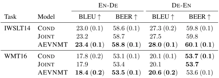
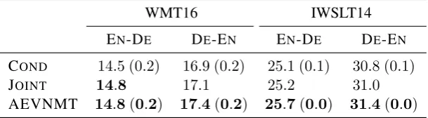
4.1 Results

EN-DE DE-EN

Task Model BLEU↑ BEER↑ BLEU↑ BEER↑

IWSLT14 COND 23.0 (0.1) 58.6 (0.1) 27.3 (0.2) 59.8 (0.1) JOINT 23.2 58.7 27.5 59.8

AEVNMT 23.4(0.1) 58.8(0.1) 28.0(0.1) 60.1(0.1)

WMT16 COND 17.8 (0.2) 53.1 (0.1) 20.1 (0.1) 53.7(0.1) JOINT 17.9 53.4 20.1 53.7

AEVNMT 18.4(0.2) 53.5(0.1) 20.6(0.2) 53.6 (0.1)

Table 3: Test results for in-domain training on IWSLT (top) and NC (bottom): we report average(1std)across5

independent runs for CONDand AEVNMT, but a single run of JOINT.

we additionally report METEOR (Denkowski and Lavie,2011) and TER (Snover et al., 2006). We de-truecase and de-tokenize our system’s predic-tions and compute BLEU scores using Sacre-BLEU (Post, 2018).6 _{For BEER, METEOR and} TER, we tokenize the results and test sets using the same tokenizer as used by SacreBLEU. We make use of BEER 2.0, and for METEOR and TER use MULTEVAL (Clark et al., 2011). In Appendix D

we report validation results, in this case in terms of BLEU alone as that is what we used for model se-lection. Finally, to give an indication of the degree to which results are sensitive to initial conditions (e.g. random initialisation of parameters), and to avoid possibly misleading signifiance testing, we report the average and standard deviation of5 in-dependently trained models. To spare resources we do not report multiple runs for JOINT, but our experience is that its performance varies similarly to that of the conditional baseline.

We start with the case where we can reasonably assume training data to be in-domain with respect to test data. Table3shows in-domain training per-formance. First, we remark that our conditional baseline for the IWSLT14 task (IWSLT training) is very close to an external baseline trained on the same data (Bahdanau et al., 2017).7 The results on IWSLT show benefits from joint modelling and in particular from learning a shared latent space. For the WMT16 task (NC training), BLEU shows a similar trend, namely, joint modelling with a shared latent space (AEVNMT) outperforms both conditional modelling and the simple joint model.

6_{Version string: BLEU+case.mixed+numrefs.1+}

smooth.exp+tok.13a+version.1.2.12

7_{Bahdanau et al.(2017) report27.56on the same test set}

for DE-EN, though note that they train on words rather than BPEs and use a different implementation of BLEU.

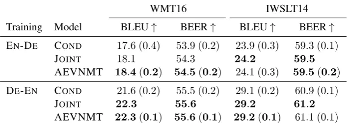
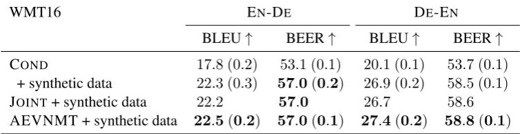
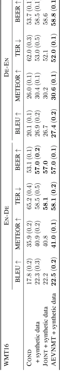
We now consider the scenario where we know for a fact that observations come from two differ-ent data distributions, which we realise by train-ing our models on a concatenation of IWSLT and NC. In this case, we perform model selection once on the concatenation of both development sets and evaluate the same model on each domain sepa-rately. We can see in Table4that conditional mod-elling is never preferred, JOINTperforms reason-ably well, especially for DE-EN, and that in every comparison our AEVNMT outperforms the condi-tional baseline both in terms of BLEU and BEER. Another common scenario where two very dis-tinct data distributions are mixed is when we capi-talise on the abundance of monolingual data and train on a concatenation of gold-standard bilin-gual data (we use NC) and synthetic bilinbilin-gual data derived from target monolingual corpora via back-translation (Sennrich et al., 2016a) (we use News Crawl). In such a scenario the latent vari-able might be vari-able to inform the translation model of the amount of noise present in the source sen-tence. Table5shows results for both baselines and AEVNMT. First, note that synthetic data greatly improves the conditional baseline, in particular translating into English. Once again AEVNMT consistently outperforms conditional modelling and joint modelling without latent variables.

WMT16 IWSLT14

Training Model BLEU↑ BEER↑ BLEU↑ BEER↑

EN-DE COND 17.6 (0.4) 53.9 (0.2) 23.9 (0.3) 59.3 (0.1) JOINT 18.1 54.3 24.2 59.5

AEVNMT 18.4(0.2) 54.5(0.2) 24.1 (0.3) 59.5(0.2)

DE-EN COND 21.6 (0.2) 55.5 (0.2) 29.1 (0.2) 60.9 (0.1) JOINT 22.3 55.6 29.2 61.2

AEVNMT 22.3(0.1) 55.6(0.1) 29.2(0.1) 61.1 (0.1)

Table 4: Test results for mixed-domain training: we report average(1std)across5independent runs for CONDand

AEVNMT, but a single run of JOINT.

it has never seen. On a dataset covering various unseen genres, we observe that both COND and AEVNMT perform considerably worse showing that without taking domain adaptation seriously both models are inadequate. In terms of BLEU, differences range from−0.3 to0.8(EN-DE) and 0.3 to 0.7 (DE-EN) and are mostly in favour of AEVNMT (17/20 comparisons).

Remarks It is intuitive to expect latent variable modelling to be most useful in settings containing high variability in the data, i.e. mixed-domain and synthetic data settings, though in our experiments AEVNMT shows larger improvements in the in-domain setting. We speculate two reasons for this: i) it is conceivable that variation in the mixed-domain and synthetic data settings are too large to be well accounted by a diagonal Gaussian; and ii) the benefits of latent variable modelling may diminish as the amount of available data grows.

4.2 Probing latent space

To investigate what information the latent space encodes we explore the idea of training simple

linear probes ordiagnostic classifiers(Alain and Bengio, 2017;Hupkes et al.,2018). With simple Bayesian logistic regression we have managed to predict from Z ∼ q(z|x) domain indicators (i.e. newswire vs transcripts) and gold-standard vs syn-thetic data at performance above 90% accuracy on development set. However, a similar perfor-mance is achieved from the deterministic average state of the bidirectional encoder of the conditional baseline. We have also been able to predict from Z ∼ q(z|x) the level of noise in back-translated data measured on the development set at the sen-tence level by an automatic metric, i.e. METEOR, with performance above what can be done with

random features. Though again, the performance is not much better than what can be done with a conditional baseline. Still, it is worth highlight-ing that these aspects are rather coarse, and it is possible that the performance gains we report in §4.1are due to far more nuanced variations in the data. At this point, however, we do not have a good qualitative assessment of this conjecture.

5 Related Work

Joint modelling In similar work,Shah and Bar-ber(2018) propose a joint generative model whose probabilistic formulation is essentially identical to ours. Besides some small differences in archi-tecture, our work differs in two regards: motiva-tion and strategy for predicmotiva-tions. Their goal is to jointly learn from multiple language pairs by shar-ing a sshar-ingle polyglot architecture (Johnson et al.,

2017). Their strategy for prediction is based on a form of stochastic hill-climbing, where they sam-ple an initial z from the standard Gaussian prior and decode via beam search in order to obtain a draft translation y˜ = greedy_yP(y|z, x).This translation is then iteratively refined by encoding the pair hx,y˜i, re-sampling z, though this time fromq(z|x,y˜), and re-decoding with beam search. Unlike our approach, this requires multiple calls to the inference network and to beam search. More-over, the inference model, which is trained on gold-standard observations, is used on noisy tar-get sentences.

Cotterell and Kreutzer (2018) interpret back-translation as a single iteration of a wake-sleep al-gorithm (Hinton et al.,1995) for a joint model of bitext P(x, y|θ) = P(y|x, θ)P?(x). They

sam-ple directly from the data distributionP?(x) and

WMT16 EN-DE DE-EN

BLEU↑ BEER↑ BLEU↑ BEER↑

COND 17.8 (0.2) 53.1 (0.1) 20.1 (0.1) 53.7 (0.1) + synthetic data 22.3 (0.3) 57.0(0.2) 26.9 (0.2) 58.5 (0.1) JOINT+ synthetic data 22.2 57.0 26.7 58.6 AEVNMT + synthetic data 22.5(0.2) 57.0(0.1) 27.4(0.2) 58.8(0.1)

Table 5: Test results for training on NC plus synthetic data (back-translated News Crawl): we report average(1std)

across5independent runs for CONDand AEVNMT, but a single run of JOINT.

on a separate objective. Zhang et al.(2018) pro-pose a joint model of bitext trained to incorporate the back-translation heuristic as a trainable com-ponent in a formulation similar to that ofCotterell and Kreutzer (2018). In both cases, joint mod-elling is done without a shared latent space and without a source language model.

Multi-task learning An alternative to joint learning is to turn to multi-task learning and ex-plore parameter sharing across models trained on different, though related, data with different ob-jectives. For example,Cheng et al.(2016) incor-porate both source and target monolingual data by multi-tasking with a non-differentiable auto-encoding objective. They jointly train a source-to-target and source-to-target-to-source system that act as en-coder and deen-coder respectively. Zhang and Zong

(2016) combine a source language model objec-tive with a source-to-target conditional NMT ob-jective and shared the source encoder in a multi-task learning fashion.

Variational LMs and NMT Bowman et al.

(2016) first proposed to augment a neural lan-guage model with a prior over latent space. Our source component is an instance of their model. More recently, Xu and Durrett (2018) proposed to use a hyperspherical uniform prior rather than a Gaussian and showed the former leads to bet-ter representations. Zhang et al.(2016) proposed the first VAE for NMT. They augment the condi-tional with a Gaussian sentence embedding and model observations as draws from the marginal P(y|x, θ) =R

p(z|x, θ)P(y|x, z, θ)dz. Their for-mulation is a conditional deep generative model (Sohn et al.,2015) that does not model the source side of the data, where, rather than a fixed standard Gaussian, the latent model is itself parameterised and depends on the data. Schulz et al. (2018) extend the model of Zhang et al. (2016) with a

Markov chain of latent variables, one per timestep, allowing the model to capture greater variability.

Latent domains In the context of statistical MT,

Cuong and Sima’an (2015) estimate a joint dis-tribution over sentence pairs while marginalising discrete latent domain indicators. Their model fac-torises over word alignments and is not used di-rectly for translation, but rather to improve word and phrase alignments, or to perform data selec-tion (Hoang and Sima’an, 2014), prior to train-ing. There is a vast literature on domain adap-tation for statistical machine translation (Cuong and Sima’an,2017), as well as for NMT (Chu and Wang,2018), but a full characterisation of this ex-citing field is beyond the scope of this paper.

6 Discussion and Future Work

We have presented a joint generative model of translation data that generates both observations conditioned on a shared latent representation. Our formulation leads to questions such as why joint learning? andwhy latent variable modelling? to which we give an answer based on statistical facts about conditional modelling and marginalisation as well as empirical evidence of improved perfor-mance. Our model shows moderate but consis-tent improvements across various settings and over multiple independent runs.

Acknowledgements

This project has received fund-ing from the Dutch Organiza-tion for Scientific Research VICI Grant No 277-89-002 and from the European Union’s Horizon 2020 research and innovation programme under grant agreement No 825299 (GoURMET). We also thank Philip Schulz, Khalil Sima’an, and Joost Bastings for comments and helpful discussions. A Titan Xp card used for this research was donated by the NVIDIA Corporation.

References

G. Alain and Y. Bengio. 2017. Understanding

interme-diate layers using linear classifier probes. InICLR,

2017, Toulon, France.

A. Alemi, B. Poole, I. Fischer, J. Dillon, R. A. Saurous,

and K. Murphy. 2018. Fixing a broken ELBO. In

Proceedings of ICML, 2018, pages 159–168, Stock-holm, Sweden.

D. Bahdanau, P. Brakel, K. Xu, A. Goyal, R. Lowe, J. Pineau, A. Courville, and Y. Bengio. 2017. An

actor-critic algorithm for sequence prediction. In

ICLR, 2017, Toulon, France.

D. Bahdanau, K. Cho, and Y. Bengio. 2015. Neural

Machine Translation by Jointly Learning to Align and Translate. InICLR, 2015, San Diego, USA.

D. M. Blei, A. Kucukelbir, and J. D. McAuliffe. 2017. Variational inference: A review for statisticians.

JASA, 112(518):859–877.

O. Bojar, R. Chatterjee, C. Federmann, Y. Graham, B. Haddow, S. Huang, M. Huck, P. Koehn, Q. Liu, V. Logacheva, C. Monz, M. Negri, M. Post, R.

Ru-bino, L. Specia, and M. Turchi. 2017.

Find-ings of the 2017 conference on machine translation (wmt17). InProceedings of WMT, 2017, pages 169– 214, Copenhagen, Denmark.

O. Bojar, R. Chatterjee, C. Federmann, Y. Graham, B. Haddow, M. Huck, A. Jimeno Yepes, P. Koehn, V. Logacheva, C. Monz, M. Negri, A. Neveol, M. Neves, M. Popel, M. Post, R. Rubino, C. Scarton, L. Specia, M. Turchi, K. Verspoor, and M. Zampieri.

2016. Findings of the 2016 conference on machine

translation. In Proceedings of WMT, 2016, pages 131–198, Berlin, Germany.

L. Bottou and Y. L. Cun. 2004. Large scale online learning. In S. Thrun, L. K. Saul, and B. Sch¨olkopf,

editors, NIPS, 2004, pages 217–224. Vancouver,

Canada.

S. R. Bowman, L. Vilnis, O. Vinyals, A. Dai, R. Joze-fowicz, and S. Bengio. 2016. Generating sentences

from a continuous space. InProceedings of CoNLL,

2016, pages 10–21, Berlin, Germany.

M. Cettolo, J. Niehues, S. St¨uker, L. Bentivogli, and M. Federico. 2014. Report on the 11th iwslt

eval-uation campaign, iwslt 2014. In Proceedings of

IWSLT, 2014, Lake Tahoe, USA.

Y. Cheng, W. Xu, Z. He, W. He, H. Wu, M. Sun, and

Y. Liu. 2016. Semi-supervised learning for neural

machine translation. InProceedings of ACL, 2016, pages 1965–1974, Berlin, Germany.

K. Cho, B. van Merrienboer, D. Bahdanau, and Y.

Ben-gio. 2014a. On the Properties of Neural Machine

Translation: Encoder-Decoder Approaches. In Pro-ceedings of SSST, 2014, pages 103–111, Doha, Qatar.

K. Cho, B. van Merrienboer, C. Gulcehre, D. Bah-danau, F. Bougares, H. Schwenk, and Y. Bengio.

2014b. Learning phrase representations using rnn

encoder–decoder for statistical machine translation. InProceedings of EMNLP, 2014, pages 1724–1734, Doha, Qatar.

C. Chu and R. Wang. 2018. A survey of domain

adap-tation for neural machine translation. In Proceed-ings of COLING, 2018, pages 1304–1319, Santa Fe, USA.

J. H. Clark, C. Dyer, A. Lavie, and N. A. Smith.

2011. Better hypothesis testing for statistical

ma-chine translation: Controlling for optimizer instabil-ity. InProceedings of ACL, 2011, pages 176–181, Portland, USA.

R. Cotterell and J. Kreutzer. 2018. Explaining and

generalizing back-translation through wake-sleep. arXiv preprint arXiv:1806.04402.

H. Cuong and K. Sima’an. 2015. Latent domain word

alignment for heterogeneous corpora. In Proceed-ings of NAACL-HLT, 2015, pages 398–408, Denver, Colorado.

H. Cuong and K. Sima’an. 2017. A survey of domain

adaptation for statistical machine translation.

Ma-chine Translation, 31(4):187–224.

H. Cuong, K. Sima’an, and I. Titov. 2016.Adapting to

all domains at once: Rewarding domain invariance in smt.TACL, 4:99–112.

M. Denkowski and A. Lavie. 2011. Meteor 1.3:

Auto-matic metric for reliable optimization and evaluation of machine translation systems. In Proceedings of WMT, 2011, pages 85–91, Edinburgh, Scotland.

I. Higgins, L. Matthey, A. Pal, C. Burgess, X. Glo-rot, M. Botvinick, S. Mohamed, and A. Lerchner.

2017. beta-VAE: Learning basic visual concepts

with a constrained variational framework. InICLR,

2017, Toulon, France.

G. E. Hinton, P. Dayan, B. J. Frey, and R. M. Neal. 1995. The” wake-sleep” algorithm for unsupervised

neural networks. Science, 268(5214):1158–1161.

C. Hoang and K. Sima’an. 2014. Latent domain

translation models in mix-of-domains haystack. In Proceedings of COLING, 2014, pages 1928–1939, Dublin, Ireland.

D. Hupkes, S. Veldhoen, and W. Zuidema. 2018. Visu-alisation and ‘diagnostic classifiers’ reveal how re-current and recursive neural networks process

hier-archical structure. JAIR, 61:907–926.

M. Johnson, M. Schuster, Q. Le, M. Krikun, Y. Wu, Z. Chen, N. Thorat, F. a. Vi´egas, M. Watten-berg, G. Corrado, M. Hughes, and J. Dean. 2017. Google’s multilingual neural machine translation system: Enabling zero-shot translation. TACL, 5:339–351.

M. Jordan, Z. Ghahramani, T. Jaakkola, and L. Saul. 1999. An introduction to variational methods for

graphical models. Machine Learning, 37(2):183–

233.

N. Kalchbrenner and P. Blunsom. 2013. Recurrent

continuous translation models. In Proceedings of EMNLP, 2013, pages 1700–1709, Seattle, USA.

D. P. Kingma and J. Ba. 2015. Adam: A method for

stochastic optimization. InICLR, 2015, San Diego,

USA.

D. P. Kingma and M. Welling. 2014. Auto-encoding

variational bayes. InICLR, 2014, Banff, Canada.

P. Koehn, H. Hoang, A. Birch, C. Callison-Burch, M. Federico, N. Bertoldi, B. Cowan, W. Shen, C. Moran, R. Zens, C. Dyer, O. Bojar, A. Constantin,

and E. Herbst. 2007. Moses: open source toolkit

for statistical machine translation. InProceedings of ACL, 2007, pages 177–180, Prague, Czech Re-public.

D. Koller and N. Friedman. 2009.Probabilistic

Graph-ical Models. MIT Press.

A. Kucukelbir, D. Tran, R. Ranganath, A. Gelman, and

D. M. Blei. 2017. Automatic differentiation

varia-tional inference.JMLR, 18(1):430–474.

M. Luong, E. Brevdo, and R. Zhao. 2017.

Neu-ral machine translation (seq2seq) tutorial.

https://github.com/tensorflow/nmt.

Y. Miao, L. Yu, and P. Blunsom. 2016. Neural

varia-tional inference for text processing. InICML, 2016,

pages 1727–1736, New York, USA.

T. Mikolov, M. Karafi´at, L. Burget, J. ˇCernock`y, and

S. Khudanpur. 2010. Recurrent neural network

based language model. In ISCA, 2010, Kyoto,

Japan.

V. Nair and G. E. Hinton. 2010. Rectified linear units

improve restricted boltzmann machines. In

Pro-ceedings of ICML, 2010, Haifa, Israel.

K. Papineni, S. Roukos, T. Ward, and W.-J. Zhu. 2002. BLEU: a method for automatic evaluation of ma-chine translation. In Proceedings of ACL, 2002, pages 311–318, Philadelphia, USA.

M. Post. 2018. A call for clarity in reporting BLEU

scores. InProceedings of WMT, 2018, pages 186– 191, Brussels, Belgium.

E. Rabinovich, R. N. Patel, S. Mirkin, L. Specia, and

S. Wintner. 2017. Personalized machine translation:

Preserving original author traits. InProceedings of EACL, 2017, pages 1074–1084, Valencia, Spain.

M. Ranzato, S. Chopra, M. Auli, and W. Zaremba. 2016. Sequence level training with recurrent neural

networks. InICLR, 2016, San Juan, Puerto Rico.

D. J. Rezende, S. Mohamed, and D. Wierstra. 2014. Stochastic backpropagation and approximate infer-ence in deep generative models. InProceedings of ICML, 2014, 2, pages 1278–1286, Bejing, China.

H. Robbins and S. Monro. 1951. A stochastic

approxi-mation method.Ann. Math. Statist., 22(3):400–407.

D. E. Rumelhart, G. E. Hinton, and R. J. Williams. 1986. Parallel distributed processing: Explorations

in the microstructure of cognition, vol. 1. Nature,

323.

J. Schulman, N. Heess, T. Weber, and P. Abbeel. 2015. Gradient estimation using stochastic computation

graphs. InNIPS, 2015, pages 3528–3536. Montreal,

Canada.

P. Schulz, W. Aziz, and T. Cohn. 2018. A stochastic

decoder for neural machine translation. In

Proceed-ings of ACL, 2018, Melbourne, Australia.

R. Sennrich, A. Birch, A. Currey, U. Germann, B. Haddow, K. Heafield, A. V. Miceli Barone, and

P. Williams. 2017. The university of edinburgh’s

neural mt systems for wmt17. In Proceedings of WMT, 2017, pages 389–399, Copenhagen, Den-mark.

R. Sennrich, B. Haddow, and A. Birch. 2016a.

Improv-ing neural machine translation models with mono-lingual data. In Proceedings of ACL, 2016, pages 86–96, Berlin, Germany.

R. Sennrich, B. Haddow, and A. Birch. 2016b.

H. Shah and D. Barber. 2018. Generative neural machine translation. In S. Bengio, H. Wallach, H. Larochelle, K. Grauman, N. Cesa-Bianchi, and

R. Garnett, editors,NIPS, 2018, pages 1352–1361.

Montreal, Canada.

N. A. Smith. 2011. Linguistic Structure Prediction.

Morgan and Claypool.

M. Snover, B. J. Dorr, R. Schwartz, L. Micciulla, and J. Makhoul. 2006. A study of translation edit rate

with targeted human annotation. Proceedings of

AMTA, 2006, pages 223 – 231.

K. Sohn, H. Lee, and X. Yan. 2015. Learning struc-tured output representation using deep conditional

generative models. In NIPS, 2015, pages 3483–

3491, Montreal, Canada.

C. K. Sønderby, T. Raiko, L. Maaløe, S. K. Sønderby,

and O. Winther. 2016. Ladder variational

au-toencoders. In NIPS, 2016, pages 3738–3746,

Barcelona, Spain.

A. Srivastava and C. Sutton. 2017. Autoencoding

vari-ational inference for topic models. InICLR, 2017,

Toulon, France.

N. Srivastava, G. Hinton, A. Krizhevsky, I. Sutskever,

and R. Salakhutdinov. 2014. Dropout: A simple

way to prevent neural networks from overfitting.

JMLR, 15:1929–1958.

M. Stanojevi´c and K. Sima’an. 2014. Fitting sentence

level translation evaluation with many dense fea-tures. InProceedings of EMNLP, 2014, pages 202– 206, Doha, Qatar.

I. Sutskever, O. Vinyals, and Q. V. V. Le. 2014. Sequence to sequence learning with neural net-works. In Z. Ghahramani, M. Welling, C. Cortes,

N. Lawrence, and K. Weinberger, editors, NIPS,

2014, pages 3104–3112. Montreal, Canada.

J. Xu and G. Durrett. 2018. Spherical latent spaces

for stable variational autoencoders. InProceedings of EMNLP, 2018, pages 4503–4513, Brussels, Bel-gium.

B. Zhang, D. Xiong, j. su, H. Duan, and M. Zhang.

2016. Variational neural machine translation. In

Proceedings of EMNLP, 2016, pages 521–530, Austin, USA.

J. Zhang and C. Zong. 2016. Exploiting source-side

monolingual data in neural machine translation. In Proceedings of EMNLP, 2016, pages 1535–1545, Austin, Texas.

Z. Zhang, S. Liu, M. Li, M. Zhou, and E. Chen. 2018. Joint training for neural machine translation mod-els with monolingual data. InProceedings of AAAI,

A Architectures

Here we describe parameterisation of the different models presented in §3. Rather than completely specifying standard blocks, we use the notation block(inputs;parameters), where we give an indi-cation of the relevant parameter set. This makes it easier to visually track which model a component belongs to.

A.1 Source Language Model

The source language model consists of a sequence of categorical draws fori= 1, . . . ,|x|

Xi|z, x<i ∼Cat(gθ(z, x<i)) (13)

parameterised by a single-layer recurrent neural network using GRU units:

fi = emb(xi;θemb-x) (14a) h0 = tanh(affine(z;θinit-lm)) (14b)

hi = GRU(hi−1,fi−1;θgru-lm) (14c)

gθ(z, x<i) = softmax(affine(hi;θout-x)). (14d)

We initialise the GRU cell with a transformation (14b) of the stochastic encodingz. For the simple joint model baseline we initialise the GRU with a vector of zeros as there is no stochastic encoding we can condition on in that case.

A.2 Translation Model

The translation model consists of a sequence of categorical draws forj= 1, . . . ,|y|

Yj|z, x, y<j ∼Cat(fθ(z, x, y<j)) (15)

parameterised by an architecture that roughly fol-lowsBahdanau et al.(2015). The encoder is a bidi-rectional GRU encoder (16b) that shares source embeddings with the language model (14a) and is initialised with its own projection of the latent representation put through atanhactivation. The decoder, also initialised with its own projection of the latent representation (16d), is a single-layer re-current neural network with GRU units (16f). At any timestep the decoder is a function of the pre-vious state, prepre-vious output word embedding, and a context vector. This context vector (16e) is a weighted average of the bidirectional source en-codings, of which the weights are computed by a Bahdanau-style attention mechanism. The output of the GRU decoder is projected to the target vo-cabulary size and mapped to the simplex using a

softmax activation (17) to obtain the categorical parameters:

s0= tanh(affine(z;θinit-enc)) (16a) sm₁ = BiGRU(f₁m,s0;θbigru-x) (16b)

ej = emb(yj;θemb-y) (16c)

t0= tanh(affine(z;θinit-dec)) (16d)

cj = attention(sm1 ,tj−1;θbahd) (16e)

tj = GRU(tj−1,[cj,ej−1];θgru-dec), (16f)

and

fθ(z, x, y<j) = softmax(affine([tj,ej−1,cj];θout-y)). (17) In baseline models, recurrent cells are initialised with a vector of zeros as there is no stochastic en-coding we can condition on.

A.3 Inference Network

The inference model q(z|x, y, λ) is a diagonal Gaussian

Z|x, y∼ N(u,diag(ss)) (18)

whose parameters are computed by an inference network. We use two bidirectional GRU encoders to encode the source and target sentences sepa-rately. To spare memory, we reuse embeddings from the generative model (19a-19b), but we pre-vent updates to those parameters based on gradi-ents of the inference network, which we indicate with the functiondetach. To obtain fixed-size rep-resentations for the sentences, GRU encodings are averaged (19c-19d) .

f₁m= detach(emb(xm₁ ;θemb-x)) (19a)

en₁ = detach(emb(yn₁;θemb-y)) (19b)

hx= avg BiGRU f1m;λgru-x

(19c) hy = avg BiGRU en1;λgru-y

(19d) hxy = concat(hx,hy) (19e)

hu= ReLU(affine(hxy;λu-hid)) (19f)

hs= ReLU(affine(hxy;λs-hid) (19g)

u= affine(hu;λu-out) (19h) s= softplus(affine(hs;λs-out)) (19i)

We use a concatenationhxy of the average source

live inRdand therefore call for linear output acti-vations (19h), whereas scales live inRd>0 and call for strictly positive outputs (19i), we follow Ku-cukelbir et al.(2017) and usesoftplus. The com-plete set of parameters used for inference is thus λ={λgru-x, λgru-y, λu-hid, λu-out, λs-hid, λs-out}.

A.4 Prediction Network

The prediction network parameterises our pre-diction model r(z|x, φ), a variant of the infer-ence model that conditions on the source sentinfer-ence alone. In §4 we explore several variants of the ELBO using different parameterisations ofrφ. In

the simplest case we do not condition on the target sentence during training, thus we can use the same network both for training and prediction. The net-work is similar to the one described inA.3, except that there is a single bidirectional GRU and we use the average source encoding (19c) as input to the predictors foruands(20c-20d).

hu= ReLU(affine(hx;λu-hid)) (20a)

hs= ReLU(affine(hx;λs-hid)) (20b) u= affine(hu;λu-out) (20c)

s= softplus(affine(hs;λs-out)) (20d)

In all other cases we use q(z|x, y, λ) parame-terised as discussed inA.3for training, and design a separate network to parameteriserφ for

tion. Much like the inference model, the predic-tion model is a diagonal Gaussian

Z|x∼ N(ˆu,diag(ˆsˆs)) (21)

also parameterised byd-dimensional location and scale vectors, however in predictinguˆandˆs(22d

-22e) it can only access an encoding of the source (22a).

hx = avg BiGRU f1m;φgru-x

(22a)

hu = ReLU(affine(hx;φu-hid)) (22b) hs = ReLU(affine(hx;φs-hid)) (22c)

ˆ

u= affine(hu;φu-out) (22d)

ˆs= softplus(affine(hs;φs-out)) (22e)

The complete set of parameters is then φ = {φgru-x, φu-hid, φu-out, φs-hid, φs-out}. For the deter-ministic variant, we useuˆ(22d) alone to approxi-mateu(19h), i.e. the posterior mean ofZ.

B Graphical models

Figure1is a graphical depiction of our AEVNMT model. Circled nodes denote random variables while uncircled nodes denote deterministic quan-tities. Shaded random variables correspond to ob-servations and unshaded random variables are la-tent. The plate denotes a dataset of |D| observa-tions.

y x

θ

z

|D|

(a) Generative model

y x

z _λ

|D|

(b) Inference model

Figure 1: On the left we have AEVNMT, a generative model parameterised by neural networks. On the right we show an independently parameterised model used for approximate posterior inference.

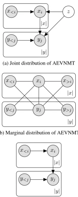
In Figure 2a, we illustrate the precise statisti-cal assumptions of AEVNMT. Here plates iterate over words in either the source or the target sen-tence. Note that the arrow fromxitoyjstates that

the jth target word depends on all of the source sentence, not on the ith source word alone, and that is the case because xi is within the source

plate. In Figure 2b, we illustrate the statistical dependencies induced in the marginal distribution upon marginalisation of latent variables. Recall that the marginal is the distribution which by as-sumption produced the observed data. Now com-pare that to the distribution modelled by the sim-ple JOINTmodel (Figure2c). Marginalisation in-duces undirected dependencies amongst random variables creating more structure in the marginal distribution. In graphical models literature this is known as moralisation (Koller and Friedman,

xi x<i

yj

y<j

z

|x|

|y|

(a) Joint distribution of AEVNMT

yj

y<j y>j

xi

x<i x>i

|x|

|y|

(b) Marginal distribution of AEVNMT

xi

x<i

yj

y<j

|x|

|y|

(c) Joint distribution modelled without latent variables

Figure 2: Here we zoom in into the model of Figure1a

to show the statistical dependencies between observed variables. In the joint distribution (top), we have the directed dependency of a source word on all of the pre-vious source words, and similarly, of a target word on all of the previous target words in addition to the com-plete source sentence. Besides, all observations depend

directly on the latent variableZ. Marginalisation ofZ

(middle) ties all variables together through undirected connections. At the bottom we show the distribution we get if we model the data distribution directly with-out latent variables.

C Robustness to out-of-domain data

We use our stronger models, those trained on gold-standard NC bilingual data and synthetic News data, to translate test sets in various unseen gen-res. These data sets are collected and distributed by TAUS,8and have been used in scenarios of ada-pation to all domains at once (Cuong et al.,2016). Table6shows the performance of AEVNMT and the conditional baseline. The first thing to note is the remarkable drop in performance showing that without taking domain adaptation seriously both models are inadequate. In terms of BLEU, differences range from−0.3 to0.8 (EN-DE) and 0.3 to 0.7 (DE-EN) and are mostly in favour of AEVNMT, though note the increased standard de-viations.

8_{TAUS Hardware, TAUS Software, TAUS Industrial}

D Validation results

WMT16 IWSLT14

EN-DE DE-EN EN-DE DE-EN

COND 14.5 (0.2) 16.9 (0.2) 25.1 (0.1) 30.8 (0.1)

JOINT 14.8 17.1 25.2 31.0 AEVNMT 14.8(0.2) 17.4(0.2) 25.7(0.0) 31.4(0.0)

Table 7: Validation results reported in BLEU for in-domain training on NC and IWSLT: we report average(1std)

across5independent runs for CONDand AEVNMT, but a single run of JOINT.

WMT & IWSLT EN-DE DE-EN

COND 20.5 (0.1) 25.9 (0.1)

JOINT 20.7 26.1

AEVNMT 20.8(0.1) 26.1(0.1)

Table 8: Validation results reported in BLEU for mixed-domain training: we report average(1std)across5

inde-pendent runs for CONDand AEVNMT, but a single run of JOINT. The validation set used is a concatenation of

the development sets from WMT and IWSLT.

WMT16 EN-DE DE-EN

COND 14.5 (0.2) 16.9 (0.2)

+ synthetic data 17.4 (0.1) 21.8 (0.1) JOINT+ synthetic data 17.3 21.8

AEVNMT + synthetic data 17.6(0.1) 22.1(0.1)

Table 9: Validation results reported in BLEU for training on NC plus synthetic data: we report average(1std)