Munich Personal RePEc Archive
House Prices and Monetary Policy
Brito, Paulo and Marini, Giancarlo and Piergallini,
Alessandro
2 January 2016
Online at
https://mpra.ub.uni-muenchen.de/89577/
House Prices and Monetary Policy
∗
Paulo Brito
†, Giancarlo Marini
‡, Alessandro Piergallini
§January 2, 2016
Abstract
This paper analyzes global dynamics in an overlapping generations general
equilibrium model with housing-wealth effects. It demonstrates that monetary
policy cannot burst rational bubbles in the housing market. Under monetary
policy rules of the Taylor-type, there exist global self-fulfilling paths of house
prices along a heteroclinic orbit connecting multiple equilibria. From bifurcation
analysis, the orbit features a boom (bust) in house prices when monetary policy
is more (less) active. The paper also proves that booms or busts cannot be ruled
out by interest-rate feedback rules responding to both inflation and house prices.
JEL Classification: C61; C62; E31; E52.
Keywords: House Prices; Housing-Wealth Effects; Monetary Policy Rules;
Equi-librium Dynamics; Global Determinacy; Heteroclinic Orbits.
∗We are very grateful to an anonymous referee for many valuable comments and remarks. We
also thank Paolo Canofari, Andrea Ferrero, Maurizio Fiaschetti, Ricardo Reis and participants to the 6th Annual Conference of the Portuguese Economic Journal, University of Porto, to the 54th Annual Conference of the Italian Economic Association, University of Bologna, and to the 2nd Macro Banking and Finance Workshop, University of Rome Tor Vergata, for very useful comments and suggestions. We gratefully acknowledge financial support from MIUR (Ministero dell’Istruzione, dell’Universit`a e della Ricerca) and FCT (Funda¸c˜ao para a Ciˆencia e a Tecnologia). The usual disclaimers apply.
†Department of Economics, Universidade de Lisboa, ISEG and UECE, Rua Miguel Lupi, 20,
1249-078 Lisbon, Portugal. UECE (Research Unit on Complexity and Economics) is financially supported from national funds by FCT (Funda¸c˜ao para a Ciˆencia e a Tecnologia), Portugal. This article is part of Strategic Project PEst-OE/EGE/UI0436/2011.
‡Department of Economics, Law and Institutions, Tor Vergata University, Via Columbia 2, 00133
Rome, Italy.
§Corresponding Author: Department of Economics and Finance, Tor Vergata University, Via
1
Introduction
The interaction between monetary policy and house prices is a central topic for current
policy-oriented macroeconomic analysis, but still under-investigated in the context of
general equilibrium models whereby nonlinear dynamics are explicitly considered. The
objective of this paper is to characterize analytically global house-price dynamics under
alternative monetary policy regimes in an overlapping generations setting that exhibits
housing-wealth effects on aggregate consumption.
Theoretical developments in monetary economics over the last decades have focused
on monetary policy rules capable of ensuring macroeconomic stability. Since the
in-flationary experience of the 1970s, central banks and academics have tried to design
simple rules that promote the credibility and transparency of monetary policy-making.
Since the seminal work by Taylor (1993), a large body of research has emphasized
the stabilizing properties of active monetary policy rules, whereby the central bank
responds to increases in inflation with a more than one-to-one increase in the nominal
interest rate.1 Empirical studies have shown that an active monetary policy stance
mimics the Federal Reserve’s behavior after 1979, over the Volcker-Greenspan period
(e.g., Judd and Rudebush, 1998; Taylor, 1999b; Clarida, Gal´ı and Gertler, 2000). 2
More recently, however, Meltzer (2011) and Taylor (2012) advocate a distinction
between a “rules-based era”, from 1985 to 2003, and an “ad hoc era”, from 2003
onwards. Over the rules-based era, a period characterized by inflation stabilization,
the Federal Reserve’s policy is well described by a simple Taylor rule whereby the
Federal Funds Rate is set as a linear function of the inflation rate and the output gap
with coefficients of 1.5 and 0.5, respectively. Over the ad hoc era, a period devastated
by the boom and bust in the housing market, the Federal Reserve’s policy deviates
from the Taylor rule.
1
See Taylor (1999a), Woodford (2003), Gal´ı (2008), and references therein.
2
In particular, from 2002 to 2006 the Federal Funds Rate was 2-3 percentage points
below the path prescribed by the Taylor rule for any period since 1980s (Poole, 2007;
Taylor, 2007). Significant downward interest-rate gaps from the Taylor rule also
oc-curred over the same period in the OECD countries as a group (Ahrend, Courn`ede and
Price, 2008).
Leamer (2007) and Taylor (2007, 2010, 2011) argue that such a “Great Deviation”
from rules-based policy making, resulting in a too accommodating monetary stance,
was a major cause of the economic and financial crisis erupted in 2007, since it triggered
boom-bust dynamics in house prices.
Could the rules-based approach to monetary policy be powerful enough to avoid
the possibility of house-price instabilities? To undertake the question analytically, in
this paper we examine the implications of the Taylor-rule framework in an overlapping
generations general equilibrium model of the type originally shown in the seminal
paper by Yaari (1965), then further developed by Blanchard (1985) and Weil (1989),
and here extended, for our purposes, in order to incorporate housing in the asset menu.
The resulting overlapping generations setting proves to be a convenient framework for
making aggregate demand sensitive to housing wealth and for formalizing transparently
the interactions between house-price dynamics and rules-based monetary policies.
We analyze the global dynamics of the model and demonstrate that the rules-based
approach relying on Taylor-style interest rate policies is powerless to burst rational
bubbles in the housing market, consisting in self-fulfilling upward trajectories in house
prices compatible with the optimal behavior by forward-looking agents. In particular,
we show that global dynamics associated to arbitrary revisions in house-price
expecta-tions typically follow a heteroclinic orbit connecting multiple equilibria.
The central point formalized in the paper is that global house-price paths
criti-cally interact with both off-target inflation paths and the stance of monetary policy.
A boom in house prices, originating in the neighborhood of the target steady state
aggregate demand and thus inflation via the positive wealth effect on aggregate
con-sumption. Under the Taylor-rule framework, which fights inflation aggressively, the
resulting increase in the real interest rate makes the economy spiral down into an
off-target decelerating-inflation path. Thus, house-price bubbles in conjunction with
the Taylor rule cause the system to converge to a liquidity trap equilibrium, with the
nominal interest rate approaching asymptotically to zero.
From bifurcation analysis, we demonstrate that the heteroclinic orbit features a
boom (bust) in house prices when monetary policy is more (less) active. Along a
liquidity-trap path, indeed, a monetary authority adopting Taylor-type prescriptions
tries to stimulate aggregate demand and therefore inflation by decreasing the nominal
interest rate more than proportionally with the decline in inflation. Nevertheless, if the
interest rate cuts are predicted to be sufficiently aggressive, house prices will increase
over time, even along a self-fulfilling decelerating-inflation trajectory.
More general specifications of the policy rules reinforce the essence of our results.
Remarkably, we prove that booms or busts cannot be ruled out by interest-rate feedback
rules responding to both inflation and house prices. In particular, we show that reacting
to house-price inflation more than to consumer-price inflation generates a basin of
attraction to the liquidity trap and even leads to local indeterminacy at the
steady-state equilibrium away from the trap.
The next Section sets forth the paper’s connections with the literature. Section 3
presents the model and the monetary regimes. Section 3 analyzes the issue of global
equilibrium dynamics under the baseline Taylor-rule framework. Section 4 extends the
analysis to the case of monetary policy rules directly reacting to house prices. Section
2
Related Literature
The present paper is linked to both empirical and theoretical literature. Empirical
evidence by Campbell and Cocco (2007), Muellbauer (2007), Dvornak and Kohler
(2007), and Carroll, Otsuka and Slacalek (2011) finds highly significant housing-wealth
effects on consumption. However, the link between house prices and consumption
dynamics is typically overlooked in standard frameworks for monetary policy analysis
(e.g., Taylor, 1999a; Woodford, 2003; Gal´ı, 2008). In this paper we intend to consider
a dynamic general equilibrium framework in which housing-wealth effects do affect the
monetary policy transmission mechanism.
Using a New Keynesian model with households’ borrowing constraints, Iacoviello
(2005) examines the role of house prices for the business cycle and the design of optimal
monetary policy.3 Consistently with the business cycle literature, the approach relies
on local dynamics, thereby abstracting from global nonlinearities and possible
multi-plicities of steady-state equilibria. This paper is different in two respects. First, we
present an alternative way to analyze the implications of house prices for monetary
pol-icy design, since we employ an overlapping generations model.4 Second, a central focus
of this paper is to depart from local analysis and focus on global nonlinear dynamics.
Therefore, following Cochrane (2011), we use the criterion of global determinacy to
evaluate the connection between monetary policy rules and macroeconomic stability.
Theoretical works by Benhabib, Groh´e and Uribe (2001, 2002) and
Schmitt-Groh´e and Uribe (2009) show that once global dynamics are taken into account, the
usual local properties of Taylor (1993, 1999b)-type interest-rate feedback rules in terms
of inflation stabilization disappear. In particular, Taylor rules give rise to multiple
self-fulfilling decelerating inflation paths converging to a long-run equilibrium around which
the monetary authority is no longer capable to ensure aggregate stability. However,
3
Further developments on the issue of optimal monetary policy in response to house-price cycles in the context of New Keynesian models can be found in Lambertini, Mendicino and Punzi (2013).
4
the framework of analysis, based on the traditional infinite-horizon representative agent
setup, diverges from our purposes, since from the standard Euler equation aggregate
demand dynamics only depend on real interest rates. The present paper contributes
to the foregoing literature in two important dimensions. First, in order to incorporate
housing-wealth effects and investigate the implied global dynamics, we shall relax the
single infinitely-lived representative agent paradigm and develop a monetary
frame-work with overlapping generations `a la Yaari (1965)-Blanchard (1985)-Weil (1989). In
this way, aggregate demand dynamics will depend not only on real interest rates, but
also on housing wealth. As a consequence, monetary policy decisions will affect
ag-gregate demand and inflation through their effects on both the real interest rate and
house prices. Our theoretical setting enables us to highlight a number of unexplored
consequences in terms of global dynamics under Taylor rules. For example, bifurcation
analysis shows that, when interest-rate feedback policies are sufficiently aggressive,
bubbles in house prices may occur even in conjunction with decelerating dynamics in
the inflation rate. Second, as a related matter, the model with housing-wealth effects
derived in this paper constitutes a useful theoretical benchmark to investigate the
dy-namic properties of monetary policy feedback rules in which the nominal interest rate
reacts not only to inflation but also to house prices.
Gal´ı (2014) shows the possible occurrence of rational bubbles in asset prices
ir-respectively of monetary policy within a two-period overlapping generations model
based on Samuelson (1958) and extended to incorporate nominal rigidities. Within
this setting, he also finds that “leaning against the wind” through real interest rate
increases in the attempt to offset a bubble in asset prices is likely to exacerbate the
bubble component itself. This feature may take place regardless of the level of asset
prices. That is, the level of asset prices could fall because of depression of the
funda-mental component despite an expanding bubble. Our investigation complements Gal´ı
(2014)’s in several important dimensions. First, the monetary version of the Yaari
paper is intended to make our analysis strictly comparable with the canonical
sin-gle infinitely-lived representative agent framework, commonly used for addressing the
dynamic effects of monetary policy rules (e.g., Benhabib, Schmitt-Groh´e and Uribe,
2001). Second, differently from Gal´ı (2014), we focus on the consequences of
house-price dynamics in a framework which explicitly account for housing-wealth effects.
Third, while Gal´ı (2014) studies the impact of monetary policy on bubble dynamics by
log-linearizing the model’s equilibrium conditions around one particular steady state
and by examining the resulting system of difference equations, the present paper is
centered on nonlinear dynamics and the existence of heteroclinic orbits connecting
dif-ferent steady states. Forth, we study equilibrium dynamics under alternative feedback
interest rate rules. From this perspective, for example, we demonstrate how reacting
to the rate of growth as opposed to the level of housing prices may critically alter both
local and global properties.
He, Wright and Zhu (2014) demonstrate the existence of bubbles in house prices in
an economic environment `a la Lagos and Wright (2005) extended to internalize liquidity
premia associated to house equity as collateral. In their model, collateral provided by
houses enables decentralized trade in the presence of incentive problems arising from
the anonymity of traders in some transactions. Importantly, the occurrence of bubbles
linked to the fact that houses expand liquidity appear to apply also in an extended
setting with money and banking. Differently from He, Wright and Zhu (2014), and
consistently with the purpose stated in the Introduction, the present paper aims to
elucidate the interactions between feedback interest rate rules of the Taylor (1993,
1999b)-style and house-price dynamics. In order to show how nonlinear dynamics can
render Taylor rules easily unable to burst rational bubbles in the housing market, we lay
out a simple continuous-time macroeconomic environment with housing-wealth effects
on aggregate demand, along the lines suggested by a fairly well-established empirical
3
The Model
Consider the following monetary version of the Yaari (1965)-Blanchard (1985)-Weil
(1989) overlapping generations setup, extended to incorporate housing in the agents’
asset menu. Each individual faces a common and constant instantaneous probability
of death, µ > 0. Population grows at a constant rate n. At each instant t a new
generation is born. The birth rate is β =n+µ. Let N(t) denote population at time
t, with N(0) = 1. So the size of the generation born at time t is βN(t) = βent, and
the size of the surviving cohort born at times ≤t isβN(s)e−µ(t−s)=βe−µteβs. Total population at time t is given by N(t) = βe−µt∫t
−∞e
βsds. As in Blanchard (1985),
there is no dynastic altruism. Financial wealth of newly born individuals is therefore
zero. Agents supply one unit of labor inelastically, which is transformed one-for-one
into output.5
The representative agent of the generation born at times≤0 chooses the time path
of consumption, c(s, t), real money balances, m(s, t), and housing, h(s, t), in order to
maximize the expected lifetime utility function given by
E0
∫ ∞
0
[
αlog Λ (c(s, t), m(s, t)) + (1−α) logh(s, t)]
e−ρtdt, (1)
where E0 is the expectation operator conditional on period 0 information, ρ > 0 is
the pure rate of time preference, and Λ (·) is a strictly increasing, strictly concave and
linearly homogenous function. Consumption and real money balances are Edgeworth
complements (Reis, 2007), that is, Λcm >0, and the elasticity of substitution between
the two is lower than unity (Cushing, 1999). Because the probability at time 0 of
surviving at timet ≥0 is e−µt, the expected lifetime utility function (1) is
∫ ∞
0
[
αlog Λ (c(s, t), m(s, t)) + (1−α) logh(s, t)]
e−(µ+ρ)tdt. (2)
5
Individuals accumulate their financial assets, a(s, t), in the form of real money
balances, interest bearing public bonds, b(s, t), and housing-wealth, q(t)h(s, t), where
q(t) is the relative house price. Therefore, a(s, t) = b(s, t) +m(s, t) +q(t)h(s, t). The
instantaneous budget constraint is given by
˙
a(s, t) = (R(t)−π(t) +µ)a(s, t) +y(s, t)−τ(s, t)−c(s, t)−
−R(t)m(s, t) +
[
˙
q(t)
q(t) −(R(t)−π(t))
]
q(t)h(s, t), (3)
whereR(t) is the nominal interest rate, π(t) is the inflation rate,τ(s, t) are real
lump-sum taxes, andµa(s, t) is an actuarial fair payment that individuals receive from a
per-fectly competitive life insurance company in exchange for their financial wealth at the
time of death, in the spirit of Yaari (1965).6 Notice that, since the asset menu includes
housing equity, in the present overlapping generations setup the Yaary-Blanchard-type
premia associated to the actuarially fair scheme imply the occurrence of reverse
mort-gage (Eschtruth and Tran, 2001).
Agents are prevented from engaging in Ponzi’s games, so that
lim
t→∞a(s, t)e
−∫0t(R(j)−π(j)+µ)dj ≥0. (4)
Letting z(s, t) denote total consumption at time t for the agent born at time s,
defined as physical consumption plus the interest forgone on real money holdings,
z(s, t) =c(s, t) +R(t)m(s, t), (5)
the individual optimizing problem can thus be solved using a two-stage procedure.7
In the first stage, consumers solve an intratemporal problem of choosing the
effi-6
Insurance companies collect financial assets from deceased individuals and pay fair premia to current generations. The presence of the life insurance market precludes the possibility for individuals of passing away leaving unintended bequests to their heirs. Assuming actuarial bonds issued by financial intermediaries would yield equivalent results. See Blanchard (1985).
7
cient allocation between consumption,c(s, t), and real money balances,m(s, t), in order
to maximize function Λ (·), for a given level of total consumption, z(s, t). Optimality
implies that the marginal rate of substitution between consumption and real money
bal-ances must equal the nominal interest rate, Λm(c(s, t), m(s, t))/Λc(c(s, t), m(s, t)) =
R(t). Because preferences are linearly homogenous, this optimality condition assumes
the following form:
c(s, t) = Γ(R(t))m(s, t), (6)
where Γ′(R)>0.
In the second stage, individuals solve an intertemporal problem of choosing the
optimal time paths of total consumption, z(s, t), and housing, h(s, t), in order to
maximize their lifetime utility function (2), given the constraints (3), (4) and the
optimal condition (6).8 Optimality yields
˙
z(s, t) = (R(t)−π(t)−ρ)z(s, t), (7)
(1−α)
α
z(s, t)
q(t)h(s, t) = (R(t)−π(t))− ˙
q(t)
q(t), (8)
lim
t→∞a(s, t)e
−∫0t(R(j)−π(j)+µ)dj = 0. (9)
Substituting the optimality condition (8) into the instantaneous budget constraint
(3), integrating forward, applying the transversality condition (9), and using the law of
motion of total consumption (7), we can express total consumption as a linear function
of total wealth:
z(s, t) =α(µ+ρ)(
a(s, t) +k(s, t))
, (10)
where k(s, t) ≡ ∫ ∞
t (y(s, t)−τ(s, t))e−
∫v
t(R(j)−π(j)+µ)djdv denotes human wealth,
de-fined as the present discounted value of after-tax labor income. From (5), (6), and
8
(10), it also follows that
c(s, t) = α(µ+ρ)
L(R(t))
(
a(s, t) +k(s, t))
. (11)
Combining next (5), (6) and (7), we obtain the optimal time path of individual
consumption:
˙
c(s, t) =
(
R(t)−π(t)−ρ− L
′(R(t))
L(R(t))R˙(t)
)
c(s, t), (12)
whereL(R)≡1+R/Γ (R) andL′(R)>0. According to (12), the optimal consumption
growth rate is identical across all generations. Function L(R) satisfies L(0) = 1,
L(∞) = +∞, L′(0) = ∞ and L′(∞) = 0. The latter properties are verified, for
example, if we assume that Λ(¯c,m¯) is a CES function.
3.1
Aggregation and Fiscal Policy
We can now derive the evolution of aggregate variables. The population aggregate for a
generic variable at individual level, x(s, t), is defined asX(t)≡βe−µt∫t
−∞x(s, t)e βsds.
The corresponding quantity in per capita terms is defined as x(t) ≡ X(t)e−nt =
β∫t
−∞x(s, t)eβ(s−t)ds.
Suppose that each agent faces identical age-independent income and tax flows, so
that y(s, t) = y(t) and τ(s, t) = τ(t), as in Blanchard (1985). Using a(t, t) = 0 and
c(t, t) = [α(µ+ρ)/L(R(t))]k(t, t), the budget constraint, the optimal time path of
consumption, the optimal time path of house prices, and the transversality condition
expressed in per capita terms are, respectively, of the form9
˙
a(t) = (R(t)−π(t)−n)a(t) +y(t)−τ(t)−c(t)−
−R(t)m(t) +
[
˙
q(t)
q(t) −(R(t)−π(t))
]
q(t)h(t), (13)
9
˙
c(t) =
(
R(t)−π(t)−ρ−L
′(R(t))
L(R(t))R˙(t)
)
c(t)−αβ(ρ+µ)
L(R(t)) a(t), (14)
˙
q(t)
q(t) = (R(t)−π(t))−
(1−α)
α
L(R(t))c(t)
q(t)h(t) , (15)
lim t→∞a(t)e
−∫0t(R(j)−π(j)+µ)dj = 0. (16)
From (14), the rate of change of per capita consumption depends on the level of financial
wealth a(t), since future cohorts’ consumption is not valued by agents currently alive.
In particular, older generations are wealthier than younger generations, and so consume
more and save less. Only in the limiting case in which the birth rateβ is equal to zero,
per capita consumption dynamics follows the standard Euler equation prevailing in the
infinitely-lived representative agent paradigm.
The flow budget constraint of the government in per capita terms is given by
˙
b(t) + ˙m(t) = (R(t)−π(t)−n)b(t)−τ(t)−π(t)m(t). (17)
To concentrate on the implications of housing-wealth effects, the government is assumed
to adopt a tax policy consisting in balancing the budget at all times. It then follows
that taxes are such that
τ(t) +π(t)m(t) = (R(t)−π(t)−n)b(t). (18)
3.2
Monetary Policy Rules
To close the model, one needs to specify the monetary policy regime. We shall
con-sider first the case in which the monetary authority follows a conventional Taylor rule,
controlling R(t) according to a feedback rule of the form
whereT(·) is a continuous, strictly increasing and strictly positive function. Monetary
policy is active when T′(π(t)) > 1 and passive when T′(π(t)) < 1. In particular, we
may assume, as advocated by Taylor (1993, 1999b), a linear rule such as
T(π(t)) = ˜r+π(t) +γ(π(t)−π˜), (20)
where ˜r and ˜π are the central bank’s targets for the real interest rate and the inflation
rate, and γ >0 is the policy parameter featuring an active monetary policy.
We shall also consider alternative rules controlling for both general price inflation
and the housing price level,
T(π(t), q(t)) = ˜r+π(t) +γ(π(t)−π˜) +ϵ(q(t)−q˜), (21)
where ˜q, ϵ >0, or controlling for both general price and housing price inflations,
T
(
π(t),q˙(t) q(t)
)
= ˜r+π(t) +γ(π(t)−π˜) +δq˙(t)
q(t), (22)
where δ >0.
3.3
Equilibrium
Total outputy(t) and housing supply ¯h(t)sare assumed to grow at the constant raten,
without loss of generality. It follows that per capita output and housing are constant
and can be normalized to one, y(t) = y = hs = 1, for analytical convenience.
Equi-librium in the goods market requires that c(t) = y = 1. Equilibrium in the housing
market requires thath(t) = hs = 1. The balanced budget rule implies ˙b(t) + ˙m(t) = 0,
so that total government liabilities are constant over time, b(t) +m(t) = l, where l is
a constant. For analytical convenience, we can study the dynamic properties of the
model normalizing the constant l to zero.
rate is given by
R(t)−π(t) = ρ+L
′(R(t))
L(R(t))R˙(t) +
αβ(ρ+µ)
L(R(t)) q(t). (23)
Then, the nominal interest rate dynamics are given by
˙
R(t) = 1
L′(R(t))[(R(t)−π(t)−ρ)L(R(t))−αβ(ρ+µ)q(t)]. (24)
From (15), house price dynamics are given by
˙
q(t) = [R(π(t))−π(t)]q(t)− (1−α)
α L[R(π(t))]. (25)
The equilibrium dynamic system is completed by introducing a monetary policy
rule. Consider a generic rule as
R(t) = T (π(t), q(t),q˙(t)/q(t)), (26)
whereT(π, q,q/q˙ ) is increasing and additively separable in all its components. We can
solve equation (26) forπ to get
π(t) = P(R(t), q(t),q˙(t)/q(t)). (27)
An active policy is such that ∂T /∂π > 1, which implies that 0< ∂P/∂R < 1 for any
(R, q,q/q˙ ). To be an equilibrium, the paths (R(t), q(t), π(t))t∈[0,∞), solving equations
(24), (25) and (27), should verify the no-Ponzi game and the transversality conditions.
4
Dynamics under the Taylor-Rule Framework
We analyze initially local and global equilibrium dynamics under the baseline
4.1
Steady-State and Local Dynamics
A generic conventional Taylor rule impliesπ =P(R) = T−1(R), where 0< P′
(R)<1.
We can rewrite the system (24)-(25) as
˙
q(t) = (R(t)−P(R(t))) (q(t)−Ψ(R(t))), (28)
˙
R(t) = αβ(ρ+µ)
L′(R(t)) (Φ(R(t))−q(t)), (29)
where
Ψ(R) ≡ (
1−α α
) (
L(R)
R−P(R)
)
, (30)
Φ(R) ≡ (
R−P(R)−ρ αβ(ρ+µ)
)
L(R). (31)
Equilibrium steady states are bounded values forR andq, such that the transversality
condition (16) holds. Hence limt→∞(R(t)−P(R(t)) +µ)>0.
Defining
r∗ ≡ ρ+ √
ρ2+ 4β(1−α) (ρ+µ)
2 (32)
and observing that r∗ > ρ >0, the following proposition holds.
Proposition 1 Assume a conventional Taylor rule in which monetary policy is globally
active. Then: (a) if P(0) ≥ 0, there is a unique steady state equilibrium (R∗, q∗) =
(R∗
1, q1∗), where
q1∗ =
(
1−α α
)
L(R∗
1)
r∗ >0, (33)
and R∗
1 = {R : R−P(R) = r∗} is the unique element; (b) if 0 > P(0) >−r∗, there
are two equilibrium steady states (0, q∗
0) and (R∗1, q∗1), where
q0∗ =− (
1−α α
)
1
P(0) >0; (34)
and (c) if P(0) ≤ −r∗, there is a unique steady state equilibrium (R∗, q∗) = (0, q∗
Proof. See Appendix C.
As a result, interest-rate feedback rules of the Taylor-type may give rise to multiple
steady-state values for house prices. The long-run inflation rates associated to the
two steady states q∗
0 and q1∗ are π0∗ = P(0) < 0 and π1∗ = P(R∗1) = R∗1 −r∗ > π0∗,
respectively.10
Compare the steady-state level of house prices associated with a zero nominal
in-terest rate, q∗
0, with the steady-state level of house prices associated with a positive
nominal interest rate, q∗
1. From Proposition 1, it follows that q0∗ > q∗1 if and only if
r∗+P(0)L(R∗
1)>0.11 The latter condition is sufficient for the existence of two steady
states, since it satisfies r∗+P(0) >0. However, if r∗ +P(0) > 0≥ r∗+P(0)L(R∗
1),
we have two steady states andq∗
0 ≤q1∗. If we assume a linear conventional Taylor rule,
the case in which q∗
0 > q1∗ occurs when
Γ
(
(1 +γ)r∗+γπ˜−r˜
γ
)
> r˜−γ˜π
γ , (35)
which tends to be verified when the long-run real interest rate r∗, the inflation target
˜
π, the elasticity of substitution between real money balances and consumption, and/or
the monetary policy feedback parameter γ are sufficiently large.
Explore now local equilibrium dynamics. Linearizing equations (28) and (29) in
the neighborhood of any point (R, q), we obtain the Jacobian
J =
R−P(R) (1−P′(R))(q−Ψ(R))−(R−P(R))Ψ′(R)
−αβL(′ρ(R+)µ)
αβ(ρ+µ)
(L′(R))2 (Φ′(R)L′(R)−(Φ(R)−q)L′′(R))
. (36)
10
For the case of a linear rule `a la Taylor (1993, 1999b), we can determineR∗
1explicitly. Substituting
equation (20) yieldsR∗
1 = (1 +γ)(P(0) +r∗)/γ=r∗+ ˜π+ (r∗−˜r)/γ, becauseP(0) = (γπ˜−r˜)/(1 +γ).
In this case, a necessary condition for the existence of two steady states is (1 +γ)r∗−γπ >˜ r > γ˜ π˜.
11
The trace and the determinant of the Jacobian matrix are
trJ =R−P(R) + αβ(ρ+µ)
L′(R)
(
Φ′(R)−(Φ(R)−q)L ′′(R)
L′(R)
)
and
detJ = αβ(ρ+µ)
L′(R)
(R−P(R))(Φ′(R)−Ψ′(R) + (q−Φ(R))L′′(R) L′(R)
)
+
+(1−P′(R))(q−Ψ(R))
.
We readily observe that
Ψ′(R) = Ψ(R)
(
L′(R)
L(R) −
1−P′(R)
R−P(R)
)
and
Φ′(R) = Φ(R)
(
1−P′(R)
R−P(R)−ρ − L′(R)
L(R)
)
.
Hence, the following proposition holds.
Proposition 2 Let the assumptions in Proposition 1 hold, such that there are two
steady state equilibria. Then, the steady state (0, q∗
0) is a singular saddle point and the
steady state (R∗
1, q1∗) is a source.
Proof. See Appendix D.
From Proposition 2, since both R(t) and q(t) are jump variables, the steady state
in which R∗ =R∗
1 > 0 is locally determinate and the steady state in which R∗ = 0 is
locally indeterminate.
As a result, even in the presence of housing-wealth effects, an active monetary
policy stance in the spirit of Taylor (1993, 1999b) exhibits the usual property of local
determinacy. In particular, in the neighborhood of (R∗
1, q1∗), and in the absence of
exogenous fundamental shocks, the only equilibrium path is R(t) =R∗
Nevertheless, in a small neighborhood around the steady state in which R∗ = 0,
local indeterminacy applies, i.e., there exist infinite equilibrium paths ofR(t) andq(t)
converging asymptotically to the steady state: for any initialR(0) there exists a q(0)
such that the time paths of R(t) andq(t) satisfying the system (28)-(29) will converge
asymptotically to that steady state. As this is a singular steady state, in the sense
that the eigenvalues for system (R, q) are infinite, the speed of approach is locally
very high. Singular steady states appear in economic theory from the existence of
static constraints in some macroeconomic models, as in Leeper and Sims (1994), and
Barnett and He (2004, 2006, 2010). However, in our case, the singularity has a different
nature: it is related to the properties of function Γ(R), since whenR tends to zero the
relationship between consumption and money demand becomes locally insensitive to
the nominal interest rate. This type of singularity seems not to have been examined
previously and can only be analyzed by investigating global dynamics.
4.2
Global Dynamics
We now conduct a global dynamics analysis of the effects of the baseline Taylor-rule
framework. Thereafter, we shall investigate whether changing the Taylor rule by
in-corporating the housing prices significantly modifies the dynamics.
Proposition 3 Let the assumptions in Proposition 1 hold, such that there are two
steady state equilibria. Then, there is a heteroclinic orbit joining steady states (R∗
1, q1∗)
and (0, q∗
0). The orbit has a positive slope near the steady state (R∗1, q∗1) and has a zero
slope near the steady state (0, q∗
0).
Proof. See Appendix E.
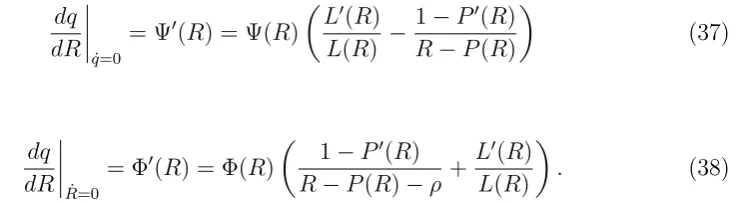
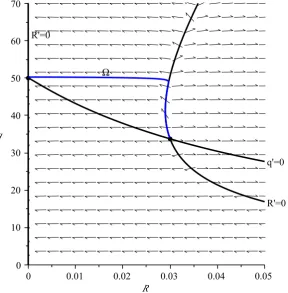
Figures 1 and 2 present the phase diagrams for the cases in whichq∗
0 > q1∗ andq0∗ <
q∗
1. In both cases, there is a heteroclinic trajectory joining the two steady states, and
this trajectory is positively sloped at the neighborhood of (R∗
1, q∗1). This implies that
Figure 1. The boom in house prices stimulates aggregate demand and thus inflation via
the positive wealth effect on aggregate consumption. However, the aggressive increase
in the real interest rate implied by the Taylor rule makes the economy spiral down
into an off-target decelerating-inflation path, leading the economy to the liquidity trap
equilibrium.
As a consequence of Proposition 3, there is not only local indeterminacy at the
steady state (q∗
0,0), but also global indeterminacy: any point along the heteroclinic
orbit is an equilibrium and, if it is not located at any of the two steady states, there is
a transition dynamics which converges asymptotically to the liquidity trap.
Next, we set out the analytical rationale for our results. The isocline ˙q = 0 has
just one branch, q = Ψ(R), while the isocline ˙R = 0 has two branches, R = 0 and
q= Φ(R). The slopes of the last two equations are, respectively,
dq dR ˙ q=0
= Ψ′(R) = Ψ(R)
(
L′(R)
L(R) −
1−P′(R)
R−P(R)
) (37) and dq dR ˙ R=0
= Φ′(R) = Φ(R)
(
1−P′(R)
R−P(R)−ρ + L′(R)
L(R)
)
. (38)
With the assumptions made at Proposition 1, the isocline ˙q = 0 has a positive value
at R = 0 and an asymptote at this point, because q = Ψ(0) > 0 if P(0) < 0 and
Ψ′(0) = Ψ(0)(L′(0) + (1−P′(0))/P(0)) = +∞. On the other side, Ψ′(∞) = 0. For
positive nominal interest rates, the slope depends upon the relationship between the
wealth effect on consumption and the monetary rule. The schedule has a negative slope
everywhere if Ψ′
(R) < 0, that is, if L′(R)/L(R) < (1−P′(R)/(R−P(R)). This is
the case depicted in Figure 1. However, if this condition does not hold, that is locally
L′(R)/L(R)>(1−P′(R)/(R−P(R)), the two isoclines are locally increasing. This is
Let us consider the following example: if the monetary rule is linear and Λ(c, m) is
a CES function,
Λ(¯c,m¯) = [ηc¯ζ−ζ1 + (1−η) ¯m ζ ζ−1
]ζ− 1 ζ
, (39)
with 0< η, ζ <1, the first case occurs if
− (
1 +γ γ
)
P(0) = ˜r−γπ˜
γ <
[
1
ξ
(
ζ
1−ζ−γ
)ζ]1/(1−ζ)
,
where ξ ≡ [η/(1−η)]1−ζ. There are two cases. First, if γ > 1−ζ, the isocline ˙q = 0 is locally increasing. Second, if γ < 1−ζ, the isocline ˙q = 0 may (not) be locally
increasing, for an active Taylor rule, if the target for the real interest rate is relatively
high (low), the target for the inflation rate is relatively low (high), and/or the degree
of reactiveness of the nominal interest rate to inflation is relatively low (high).
If the first case occurs, then we always have q∗
1 < q0∗. In the second case, we may
haveq∗
1 > q∗0, depending upon the deep parameters for the consumer demand and the
monetary rule. A necessary condition for q∗
1 > q0∗ is that locally Ψ′(R)>0.
The equilibrium pointR∗ = 0 always exists and is, geometrically, in the intersection
of isocline ˙q= 0 with the first branch of isocline ˙R= 0. The second equilibrium point,
which exists under the conditions of Proposition 1, is in the intersection of the isocline
˙
q = 0 with the second branch of the isocline ˙R = 0, whose slope is given by equation
(38). For the range in which q > 0, we have Φ(R)> 0, which means that the branch
of the isocline, in which q= Φ(R), is globally increasing. Since
Ψ(0)−Φ(0) = (P(0) +r+)(P(0) +r−)
αβ(ρ+µ)P(0) ,
where
r+ ≡
ρ+√ρ2 + 4β(1−α) (ρ+µ)
2 , r− ≡
ρ−√ρ2+ 4β(1−α) (ρ+µ)
andP(0) <0, a necessary condition for the existence of the steady state (R∗
1, q1∗), which
was introduced in Proposition 1, is P(0) +r+ > 0, implying that Ψ(0)−Φ(0) > 0,
which means that the isocline ˙q = 0 cuts the q−axis above the isocline ˙R = 0. In
Proposition 2, we proved that this steady state is locally a source.
Furthermore, we may conjecture that the unstable manifold associated to the
equi-librium point (R∗
1, q1∗) and the stable manifold associated to the equilibrium point
(0, q∗
0) intersect. The proposition proves that this conjecture is right, which means
that a heteroclinic orbit defined as
Ω≡ {
(R, q)∈ W : lim
t→∞(R(t), q(t)) = (0, q ∗
0), t→−∞lim (R(t), q(t)) = (R1∗, q1∗)
}
exists in W ⊆ R2
+. In our case, Ω corresponds to the set of all the equilibrium values
for the nominal interest rate and house prices. All other points, in W/Ω, lead to a
violation of the transversality and/or the no-Ponzi game condition.
This means that there is global indeterminacy: any initial point (R(0), q(0)) ∈ Ω
is an equilibrium point and converges asymptotically to (0, q∗
0). Condition (35) implies
that if the monetary policy is more (less) active, then the reduction of the nominal
interest rate is correlated with an increase (decrease) in the prices of houses. Along a
liquidity-trap path, in fact, the central bank adopting the Taylor-rule framework tries
to stimulate aggregate demand and thus inflation by decreasing the nominal interest
rate more than proportionally with the decline in inflation. This policy triggers a fall in
the real interest rate. If the interest rate cuts are sufficiently aggressive, house prices
will increase even along the decelerating-inflation trajectory, as it emerges from the
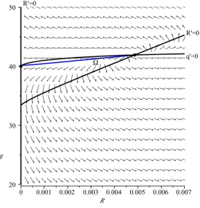
bifurcation diagram in Figure 3.
Inspection of the bifurcation diagram reveals that the above depicted global
in-determinacy result is robust with respect to alternative quarterly parameterizations,
which appear to be widely consistent with a fairly well-established empirical evidence
Clarida, Gal´ı and Gertler, 2000).
5
Dynamics under Alternative Taylor Rules
In this section we extend our analysis by examining local and global equilibrium
dy-namics for the case of Taylor rules that incorporate house prices.
5.1
Taylor Rule Depending on the Level of Housing Prices
For the case of rule (21), we have π =P(R, q), where
P(R(t), q(t)) = 1
1 +γR(t)− ϵ
1 +γq˜+P(0,0), (40)
with P(0,0)≡(γπ˜−r˜−ϵq˜)/(1 +γ).
Hence, the dynamic system assumes the form
˙
q(t) = (R(t)−P(R(t), q(t))) (q(t)−Ψ(R(t), q(t))), (41)
˙
R(t) = αβ(ρ+µ)
L′(R(t)) (Φ(R(t), q(t))−q(t)), (42)
where Ψ(R, q) and Φ(R, q) are as in equations (30) and (31), in whichP(R) is
substi-tuted by P(R, q) as in equation (40).
This case does not present substantial changes as regards the conventional Taylor
rule, as we shall see in the following Proposition.
Proposition 4 Assume a modified Taylor rule depending on the level of housing prices
as in equation (21) in which the monetary policy is active, meaning that0< ∂P/∂R <
1, and define
BP(0,0)≡ P(0,0)
2 +
[ (
P(0,0) 2
)2
+ ϵ(1−α)
α(1 +γ)
]1/2
>0.
(a) if r+ + P(0,0) ≤ B(P(0,0), then there is an unique equilibrium steady state
(R∗, q∗) = (0, q∗
0) where
q0∗ = 1 +γ
ϵ BP(0,0); (43)
(b) ifr++P(0,0)> B(P(0,0), then there are two equilibrium steady states(R∗, q∗) =
(0, q∗
0) and (R∗, q∗) = (R1∗, q1∗) where
q1∗ = (1 +γ)(P(0,0) +r+)−γR ∗
1
ϵ (44)
and
R∗1 =
{
R : L(R) =
(
α(1 +γ)r+
(1−α)ϵ
) (
P(0,0) +r+−
γ
1 +γR
)}
,
and there is a heteroclinic trajectory connecting those two equilibrium steady
states, starting from equilibrium(R∗
1, q∗1), which is locally a source, and converging
asymptotically to equilibrium (0, q∗
0).
Proof. See Appendix F.
The equilibrium (0, q∗
0) is again singular and behaves globally as a saddle point:
for R∗ = 0, we have ˙q S 0 if and only if q S q∗
0, and the vector field is horizontal on
the space W. The equilibrium steady state (R∗
1, q1∗) also displays local determinacy,
because the local Jacobian has positive eigenvalues for the admissible values of the
parameters.
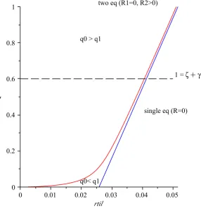
The global dynamics is as in the version of the model with a conventional Taylor rule
(see Figure 4). There is a heteroclinic orbit connecting equilibria (R1∗, q1∗) to (0, q0∗).
The only combinations of equilibrium nominal interest rates and housing prices are
those along the orbit, which means that there is global indeterminacy.
quantitatively. However, since
P(0,0) = γπ˜+ϵq˜−r˜ 1 +γ
can have any sign, although it has all parameters positive, the definition of the target
values is less stringent than in the case of the conventional Taylor rule. Furthermore,
we can exclude the case in which there is a unique steady state equilibrium (R∗
1, q1∗).
That is, the equilibrium with a zero nominal interest rate always exists.
5.2
Taylor Rule Depending on the Rate of Growth of Housing
Prices
For the case of rule (22), the inflation rate becomes a function of the rate of change of
housing prices,
π(t) = R(t) +γπ˜−˜r−δq˙(t)/q(t)
1 +γ ,
and the general equilibrium dynamic system is
˙
q(t) = γR(t) + ˜r−γπ˜
1 +γ−δ (q(t)−Ψ(R(t))), (45)
˙
R(t) = αβ(ρ+µ)
L′(R(t)) (Φ(R(t))−q(t)) +
δ
1 +γ
L(R(t))
L′(R(t)) ˙
q(t)
q(t), (46)
where Ψ(R) and Φ(R) are similar to equations (30) and (31),
Ψ ≡
(
1−α α
) (
(1 +γ)
γR+ ˜r−γπ˜
)
L(R), (47)
Φ ≡
(
γR+ ˜r−γπ˜−(1 +γ)ρ αβ(ρ+µ)(1 +γ)
)
L(R). (48)
Therefore, we can state the following proposition.
Proposition 5 Let the same assumptions as in Proposition 1 hold. Then the existence,
addition:
(a) if1 +γ > δ, then the steady state(0, q∗
0) (if it exists) is singular and is a
general-ized saddle point and the steady state (R∗
1, q1∗) (if it exists) is a source, and there
is a heteroclinic orbit joining them.
(b) if 1 +γ < δ, then the steady state (0, q∗
0) (if it exists) is singular and is a
gen-eralized sink and the steady state (R∗
1, q1∗) (if it exists) is a saddle point. If there
are two steady state equilibria, the saddle manifold associated to (R∗
1, q1∗) is the
boundary of the basin of attraction of equilibrium (0, q∗
0).
Proof. See Appendix G.
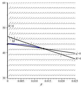
As in the version of the model with the conventional Taylor rule (see Proposition
1), the steady-state equilibria of housing prices are given in equations (34) and (33).
From now on, consider the the values for the parameters such that there are two steady
state equilibria. The associated phase diagrams are given in Figure 5, for the case in
which 1 +γ > δ, and in Figure 6, for the case in which 1 +γ < δ.
Ifδ <1 +γ, whereby the central bank reacts more to consumer-price inflation than
to house-price inflation, the global dynamics is similar to the version of the model with
a conventional Taylor rule (see Figure 5): there is global indeterminacy in the sense
that there is an interval for initial values of R, R(0) ∈ (0, R∗
1) which are equilibrium
values and the nominal interest rate tends (possibly in a non-monotonous way) to the
steady state R∗ = 0. For a given initial value of the nominal interest rate in that
interval, there is a single initial value for the equilibrium house prices. Next, the pair
(R(t), q(t)) will follow along the heteroclinic orbit Ω converging to (0, q∗
0).
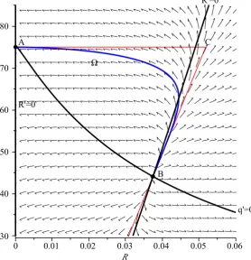
Ifδ > 1 +γ, whereby the central bank reacts more to house-price inflation than to
consumer-price inflation, the global dynamics changes substantially (see Figure 6): the
two steady-state equilibria are both locally and globally indeterminate. In particular,
the steady state (R∗
is locally indeterminate of order two. The orders of indeterminacy are given by the
dimension of the local stable manifolds. Globally, the stable sub-manifold associated to
equilibrium (R∗
1, q1∗),W1s, bounds the basin of attraction,B0, of the steady state (0, q0∗).
In our case, this means that the set B0∪W1s is the space of equilibrium states of the
economy, in the sense that all the trajectories starting in it are equilibrium trajectories.
However, if (R(0), q(0)) ∈B0, then the equilibrium trajectory will converge to (0, q0∗),
while, if (R(0), q(0)) ∈ Ws
1, then the equilibrium trajectory will converge to (R∗1, q1∗).
This means that if we have an initial nominal interest rateR(0)̸= 0, there will be one
single initial value q(0), say q1(0), such that the pair (R(t), q(t)) will converge to the
steady state (R∗
1, q∗1), but an infinite number of initial values q(0) > q1(0) such that
(R(t), q(t)) will converge to the steady state (0, q∗
0). Indeterminacy of order two indeed
implies that there is an infinite number of initial equilibrium values for q(0), given
R(0), and not just one as in the version with a conventional Taylor rule.
6
Conclusions
The alleged connection between monetary policy making and the dynamics of house
prices arguably has been one of the most debated topics in recent years. The Federal
Reserve’s accommodating monetary policy of 2002-2006 – the so-called Great Deviation
from the Taylor rule – is claimed to be responsible for the global crisis started in 2007,
since it generated boom-bust patterns in house prices. In this paper we have presented
an overlapping generations economy with housing-wealth effects and demonstrated that
house-price instabilities can well occur even if the central bank follows monetary policy
feedback rules of the Taylor-style.
We have proved that global equilibrium dynamics satisfying agents’ forward-looking
optimal choices follow, in general, a heteroclinic orbit connecting multiple steady-state
equilibria. Specifically, rules-based monetary policies, even when they aim to fight
trajectories in both house prices and inflation, which typically converge to a liquidity
trap equilibrium. Furthermore, we have demonstrated that reacting to house-price
inflation more than to consumer-price inflation gives rise to a basin of attraction to
the liquidity trap, and introduces local indeterminacy at the off-trap steady state.
Bifurcation analysis reveals that, along a liquidity-trap path, a central bank adopting
an excessively aggressive monetary policy conforming to the Taylor principle may bring
about an off-target self-fulfilling boom in house prices, even if the economy is spiraling
down into a decelerating inflation dynamics.
Therefore, the theoretical results shown in this paper provide analytical foundations
for the view that active monetary policy, per se, is not viable in order to prevent the
occurrence of bubbles in the housing market.
The framework we have examined delivers our key points in a direct way. Of course,
the analysis presented in this paper is based on simplifying assumptions needed to
render our arguments as transparent as possible.
First, we have abstracted from the presence of price stickiness. Under sticky prices,
however, the implied sluggish adjustments associated to the presence of a Phillips
curve do not alter the essence of the analysis – which is primarily focused on the
interactions between house-price dynamics and rules-based monetary policies from a
global perspective – in any fundamental dimension.
Second, we have abstracted from issues pertaining to optimal monetary policy. It is
worth emphasizing that, differently from the single infinitely-lived representative agent
paradigm, in the present overlapping generations setup the dynamics of real assets
trig-gers redistributions of wealth across generations, thereby affecting social welfare. The
implications in terms of optimal fiscal policy are analyzed by Calvo and Obstfeld (1988).
In a monetary setup, however, one should further take into account that increases in
consumer-price inflation negatively influence intergenerational equity, for they cause a
redistribution of real wealth from current to future generations. Conversely, increases
cur-rent generations. A formal analysis about the consequences of such intergenerational
features in terms of optimal monetary policy design – following the lines suggested by
Calvo and Obstefld (1988) – is beyond the scope of the present paper, and may
ar-guably constitute a challenging issue for future research. The overlapping generations
monetary setup we have presented here could then be used as a fruitful benchmark for
this purpose.
Third, we have abstracted from direct empirical estimates of the model. Empirical
questions aimed to establish, say, whether the class of models studied here actually fits
well the U.S. economy in and around 2003 when the Great Deviation took place, and
whether the quantitative requirements for global indeterminacy under the Taylor rule
– and augmented Taylor rules – were met during that period are left to future research.
A
Solution of the Consumer’s Problem
In the intertemporal optimization problem, the representative consumer born at time
schooses the optimal time path of total consumption, z(s, t), to maximize the lifetime
utility function (2), given (6) and the constraints (3) and (4). Using the definition
of total consumption, z(s, t) ≡ c(s, t) +R(t)m(s, t), and the optimal intratemporal
condition (6), we can write
log Λ (c(s, t), m(s, t)) = logυ(t) + logz(s, t), (49)
whereυ(t)≡Λ(Γ(RΓ((tR))+(t))R(t),Γ(R(t))+1 R(t))is the same for all generations. Therefore, the intertemporal optimization problem can be formalized in the following terms:
max {z(s,t), h(s,t)}
∫ ∞
0
[
α(logυ(t) + logz(s, t)) + (1−α) logh(s, t)]
subject to
˙
a(s, t) = (R(t)−π(t) +µ)a(s, t) +y(s, t)−τ(s, t)−z(s, t) +
+
[
˙
q(t)
q(t) −(R(t)−π(t))
]
q(t)h(s, t), (51)
and given a(s,0). The optimality conditions are
˙
z(s, t) = (R(t)−π(t)−ρ)z(s, t), (52)
1−α
α z(s, t) =
[
(R(t)−π(t))− q˙(t)
q(t)
]
q(t)h(s, t), (53)
lim
t→∞a(s, t)e
−∫0t(R(j)−π(j)+µ)dj = 0. (54)
Therefore, the individual budget constraint (51) can be expressed as
˙
a(s, t) = (R(t)−π(t) +µ)a(s, t) +y(s, t)−τ(s, t)−
−z(s, t) +
[
˙
q(t)
q(t)−(R(t)−π(t))
]
q(t)h(s, t)
= (R(t)−π(t) +µ)a(s, t) +y(s, t)−z(s, t)− 1−α
α z(s, t)
= (R(t)−π(t) +µ)a(s, t) +y(s, t)− 1
αz(s, t). (55)
Integrating forward (55), using the transversality condition (54) and (52), total
con-sumption turns out to be a linear function of total wealth:
z(s, t) =α(µ+ρ)(
a(s, t) +k(s, t))
, (56)
wherek(s, t) is human wealth, defined as the present discounted value of after-tax labor
income,k(s, t)≡∫ ∞
t (y(s, t)−τ(s, t))e−
∫v
t(R(j)−π(j)+µ)djdv. From (6),
where L(R(t))≡1 +R(t)/Γ (R(t)). Time-differentiating (57) yields
˙
z(s, t) = L′(R(t))c(s, t) ˙R(t) +L(R(t))˙c(s, t). (58)
Therefore, the dynamic equation for individual consumption is
˙
c(s, t) = (R(t)−π(t)−ρ)c(s, t)− L
′(R(t)) ˙R(t)
L(R(t)) c(s, t). (59)
B
Aggregation
The per capita aggregate financial wealth is given by
a(t) =β
∫ t
−∞
a(s, t)eβ(s−t)ds. (60)
Differentiating with respect to time yields
˙
a(t) =βa(t, t)−βa(t) +β
∫ t
−∞ ˙
a(s, t)eβ(s−t)ds, (61)
where a(t, t) is equal to zero by assumption. Using (3) yields
˙
a(t) = −βa(t) +µa(t) + (R(t)−π(t))a(t) +y(t)−τ(t)−c(t)−
−R(t)m(t) +
[
˙
q(t)
q(t)−(R(t)−π(t))
]
q(t)h(t)
= (R(t)−π(t)−n)a(t) +y(t)−τ(t)−c(t)−
−R(t)m(t) +
[
˙
q(t)
q(t)−(R(t)−π(t))
]
q(t)h(t). (62)
Using (11), the per capita aggregate consumption is given by
c(t) = α(µ+ρ)
where k(t) = ∫ ∞
t (y(t)−τ(t))e−
∫v
t(R(j)−π(j)+µ)djdv is the per capita aggregate human
wealth. Next differentiate with respect to time the definition of per capita aggregate
consumption, to obtain
˙
c(t) =βc(t, t)−βc(t) +β
∫ t
−∞ ˙
c(s, t)eβ(s−t)ds. (64)
Note that c(t, t) denotes consumption of the newborn generation. Since a(t, t) = 0,
from (11) we have
c(t, t) = α(µ+ρ)
L(R(t))
(
k(t, t))
. (65)
Using (12), (63) and (65) into (64) yields the time path of per capita aggregate
con-sumption:
˙
c(t) = (R(t)−π(t)−ρ)c(t)− L
′(R(t)) ˙R(t)
L(R(t)) c(t)−
αβ(ρ+µ)
L(R(t)) a(t). (66)
C
Proof of Proposition 1
Any equilibrium steady states, (R∗, q∗), are bounded points (R, q) ∈ (R
+,R++) such
that ˙q = ˙R = 0 and the transversality condition holds if R∗ −P(R∗) > −µ. From
equation (28), ˙q = 0 if and only if q = Ψ(R). From equation (29), ˙R = 0 if and only
if R = 0, because L′(0) = ∞, or q = Φ(R). Therefore, there are two candidates for
equilibrium steady states. First, we haveR = 0 andq=q∗
0 ≡Ψ(0) =−(1−α)/(αP(0))
which constitute indeed an equilibrium point only if P(0) < 0. In this case, the
transversality condition is verified, because the condition −P(0) > −µ always holds.
Second, from the condition q = Ψ(R) = Φ(R), there is a second candidate if the set
{R≥0 : Ψ(R) = Φ(R)>0} is non-empty. We have
where
r+ ≡
ρ+√
ρ2+ 4β(1−α) (ρ+µ)
2 , r− ≡
ρ−√
ρ2+ 4β(1−α) (ρ+µ)
2
andr=R−P(R)>−µfrom the transversality condition. Becauseβ(1−α) (ρ+µ)>
0, then r+ > ρ > 0 > r−. As L(R) > 1, then the condition r > ρ must hold,
which implies that the transversality condition is always met. Therefore, an equivalent
condition for the existence of a second steady state is R∗
1 = {R ≥ 0 : R−P(R) =
r+}. From the assumption that the monetary policy is globally active, R−P(R) is
monotonically increasing inR, which means thatR−P(R)∈[−P(0),+∞). Therefore,
the steady state (R∗
1, q∗1) exists if P(0) +r+ ≥ 0, where q1∗ = Ψ(R∗1) = Φ(R∗1). As a
result, there is multiplicity if 0 > P(0) ≥ −r+, there is only one steady state (R∗1, q1∗)
if P(0)>0, and there is only steady state (0, q∗
0) ifP(0) +r+ <0. We set r∗ =r+.
D
Proof of Proposition 2
For the steady-state equilibrium (R∗, q∗) = (R∗
1, q1∗), we have the trace and determinant
of the Jacobian given by
trJ(R1∗) =r∗+αβ(ρ+µ)Φ ′(R∗
1)
L′(R∗
1)
= 2r∗−ρ+(1−P ′(R∗
1)L(R∗1)
L′(R∗
1)
and
detJ(R1∗) =r∗αβ(ρ+µ)
(
Φ′(R∗
1)−Ψ′(R∗1)
L′(R∗
1)
)
= (2r
∗−ρ)(1−P′(R∗
1))L(R∗1)
(r∗−ρ)L′(R∗
1)
>0,
because
Φ′(R∗1) =q1∗
(
1−P′(R∗
1)
r∗−ρ +
L′(R∗
1)
L(R∗
1)
)
>0,
yielding the eigenvalues λ1 = 2r∗ −ρ >0 and λ2 = (1−P′(R1∗))L(R∗1)/L′(R∗1) >0 if
the monetary policy is locally active, 1−P′(R∗
is always a source.
Evaluating the trace and the determinant for equilibrium (R∗, q∗) = (0, q∗
0), with
q∗
0 = Ψ(0), we get
trJ(0) = −P(0) +αβ(ρ+µ)
(
Φ′(0)
L′(0) + (Ψ(0)−Φ(0))
L′′(0) (L′(0))2
)
and
detJ(0) =−P(0)αβ(ρ+µ)
L′(0)
(
Φ′(0)−Ψ′(0) + (Ψ(0)−Φ(0))L ′′(0)
L′(0)
)
.
As
Ψ′(0)−Φ′(0)
L′(0) = Ψ(0)−Φ(0) =
(P(0) +r+)(P(0) +r−)
αβ(ρ+µ)P(0) >0,
we have
trJ(0) = −(2P(0) +ρ) + (P(0) +r+)(P(0) +r−)
P(0)
L′′(0) (L′(0))2,
detJ(0) = (P(0) +r+)(P(0) +r−)
(
1− L
′′(0)
(L′(0))2
)
.
Recall that this steady state exists only if P(0)<0, and observe that L′(0) =∞ and
L′′(0)/(L′(0))2 =−∞. Then
trJ(0) = detJ(0) =
−∞, ifP(0) +r+>0
+∞, ifP(0) +r+<0
which means that the eigenvalues of the Jacobian are infinite and the steady state is
singular. IfP(0) +r+ >0, the steady state is multiple (case (b) in Proposition 2) and
is a kind of non-regular saddle point, and, ifP(0) +r+ <0, the steady state is unique
(case (c) in Proposition 2) and is a kind of non-regular source. In any case, the flow
approaches or diverges from (0, q∗
0) at an infinite speed and is non-differentiable locally.
In order to study local dynamics, we can use several methods, such as, first, finding
global dynamics.
If we use the first method, the natural way to remove the singularity introduced by
L′(R) at R = 0, would be to recast the system in variables (L, q),
˙
q = q(R−P(R))− (
1−α α
)
L,
˙
L = L′(R) ˙R=L(R−P(R)−ρ)−αβ(ρ+µ)q,
where L ≥1, R = R(L) is increasing and R(1) = 0, R′(1) = 0. However, in this case
there is an unique steady state (L(R∗
1), q1∗). Therefore, this method does not solve our
de-singularization problem. We use the second method in the proof of Proposition 3.
There, we show that the singular steady state (0, q∗
0), for the case P(0) +r+ >0 (i.e.,
case (b) in Proposition 2) behaves as a generalized saddle point.
E
Proof of Proposition 3
As the system (28)-(29) does not have an explicit solution, we must employ qualitative
methods in order to study global dynamics. One possible method is to find a first
integral of system (28)-(29), that is, a Lyapunov function V(.) such that V(R, q) =
constant. We could not find this function. Another method is to determine a trapping
area for the heteroclinic orbit. The rationale is the following: as the steady state
(R∗
1, q1∗) is a source, the unstable manifold is the set R+/(R∗1, q∗1); as the steady state
(0, q∗
0) is a saddle point, the stable manifold is, locally, composed by a single trajectory
belonging toR+; therefore there is an intersection of the unstable manifold of the first
point and of the stable manifold of the second which is non-empty. In order to prove
that it exists, and to characterize it, we consider a trapping area for the heteroclinic
orbit. In order to prove this, we start by determining the slopes of the heteroclinic
orbit in the neighborhoods of the two equilibria, we build a trapping area enclosing the
heteroclinic, and demonstrate that all the trajectories starting inside the trapping area
orbit.
E.1
Slopes of the Eigenspaces Associated to the Two
Equilib-ria
The unstable eigenspace Eu
1 is the tangent space to the unstable manifold associated
to equilibrium (R∗
1, q∗1), in the space where (R, q)∈ W ⊆R2+ lie,
W1u ≡ {
(R, q)∈ W : lim
t→−∞(R(t), q(t)) = (R ∗
1, q∗1)
}
.
The unstable eigenspace Eu
1 is the linear space which is tangent to W1u and is spanned
by the eigenvectors (V1,1)⊤and (V2,1)⊤ which are associated to eigenvaluesλ1 andλ2,
respectively, where
V1 =−
r+Ψ′(R∗1)
r+−ρ
, V2 =
(r+−ρ)L′(R∗1)
L(R∗
1)
.
In general, V2 > 0 and the sign of V1 is ambiguous. Observe that the the slope
of Eu
1, dRdq
Eu
1, is the opposite to the slope of isocline ˙q = 0, locally at the steady
state (R∗
1, q1∗). Let us call E1u,+ ( E1u,−) the eigenspace related to the dominant (non-dominant) eigenvalue. The following conditions can be proved: (1) if r+ > (1 −
P′(R∗
1))L(R∗1)/L′(R∗1), then 2r+−ρ > (1−P′(R∗1))L(R∗1)/L′(R∗1), which is equivalent
to λ1 > λ2, and therefore E1u,+ = {(R, q) ∈ W : (q−q1∗) = V1(R−R1∗)} and E1u,− =
{(R, q) ∈ W : (q − q∗
1) = V2(R − R∗1)}. In this case, V1 < 0 and V2 > 0 and
the slope associated to the dominant eigenvalue is negative and the slope associated
to the non-dominant eigenvalue is positive; (2) if λ1 < λ2, which is equivalent to
2r+−ρ <(1−P′(R1∗))L(R1∗)/L′(R∗1), thenr+<(1−P′(R∗1))L(R1∗)/L′(R∗1), andE1u,+ =
{(R, q)∈ W : (q−q∗
1) = V2(R−R∗1)}andE1u,− ={(R, q)∈ W : (q−q1∗) =V1(R−R∗1)}.
In this case, V1 > V2 > 0 and the slope associated to the both eigenvalues are both
positive, but the one associated with Eu
The stable manifold associated to steady state (0, q∗
0) is defined as
W0s ≡{(R, q)∈ W : lim
t→∞(R(t), q(t)) = (0, q ∗
0)
}
.
However, we saw that the projection of the steady state (0, q∗
0) in the space W is
singular. This means that the solution approaches the singular steady state
asymp-totically with an infinite speed. In order to characterize the dynamics in the spaceW
in the neighborhood of (0, q∗
0), we have to take a different approach: observe that, as
R′(1) = 0, then a na¨ıve calculation for the slope of the stable manifold in the
neigh-borhood of the singular equilibria could bedq/dR= (r+−ρ)/(αβ(ρ+µ)R′(1)) =∞.
Instead, observe that along the singular s