IMVIP 2018
IRISH MACHINE VISION AND IMAGE PROCESSING
CONFERENCE PROCEEDINGS
29
th
- 31
st
August 2018
Ulster University
Belfast, Northern Ireland
Editor:
Bryan W. Scotney
Published by the Irish Pattern Recognition & Classification Society iprcs.org
ISBN 978-0-9934207-3-3
©2018
Introduction
With IMVIP 2018 the series of Irish Machine Vision and Image Processing conferences reaches a landmark occasion: IMVIP 2018 is the 20th edition in a series of which the inaugural meeting was held at the Magee campus of Ulster University in 1997. Ulster University hosted IMVIP again in 2003 and 2008 (at the Coleraine campus) and in 2014 (at Magee). Now, in 2018, Ulster University hosts IMVIP for the fifth time, and for the first time at the Belfast campus, under the organisation of the School of Computing.
In the two decades since 1997, the IMVIP conference has been hosted throughout the island of Ireland: four times at the National University of Ireland, Maynooth (1998, 2001, 2007 and 2017), three times at Dublin City University (1999, 2006 and 2011) and at Trinity College Dublin (2004, 2009 and 2015), twice at Queen’s University Belfast (2000 and 2005) and at the National University of Ireland, Galway (2002 and 2016), and at the University of Limerick (2010).
IMVIP is established as Ireland's primary meeting for those researching in the fields of machine vision and image processing, providing a forum for the exchange of ideas and the presentation of research conducted both within Ireland and worldwide.
IMVIP is a single track conference consisting of high quality previously unpublished contributed papers focussing on both theoretical research and practical experiences in all areas of computer vision. After a rigorous review process, this year 22 papers were selected for oral presentation at the conference, with a further 10 selected for poster presentation. We thank sincerely the members of the Programme Committee for generously giving their time, effort and expertise in reviewing the submissions.
Continuing the tradition of inviting internationally-renowned experts in the theory and application of computer vision to IMVIP, we are delighted to have keynote presentations at IMVIP 2018 from Prof. Hiroshi Ishikawa, Director of the Computer Vision and Analysis Lab at Waseda University, Tokyo; Prof. Jiri Matas, Centre for Machine Perception at the Czech Technical University, Prague; and Prof. dr. Zeno Geradts, senior forensic scientist at the Netherlands Forensic Institute and Professor of Forensic Data Science at the University of Amsterdam.
IMVIP is run in association with the Irish Pattern Recognition and Classification Society (iprcs.org), a member organisation of the International Association for Pattern Recognition (IAPR) and the International Federation of Classification Societies (IFCS). In addition to IPRCS, we would like to thank the School of Computing at Ulster University for their support for and sponsorship of IMVIP 2018.
The Organising Committee extends a warm welcome to all speakers and delegates of the 20th Irish Machine Vision and Image Processing Conference, and we hope that you will thoroughly enjoy both the professional and social aspects of IMVIP 2018 in Belfast.
Director of the Computer Vision and Analysis Lab
Department of Computing and Engineering
Waseda University
Tokyo
Title: Structured Prediction by Fully Convolutional Deep Neural Networks
Centre for Machine Perception
Department of Cybernetics
Czech Technical University
Prague
Title: Multi-Class Multi-Instance Model Fitting in Computer Vision
Abstract: Many computer vision problems can be formulated as data fitting. In multi-class multi-instance fitting, the input data is interpreted as a mixture of noisy observations originating from multiple instances of multiple model types, e.g. as k lines and l circles in 2D edge maps, as k planes, l cylinders and m point clusters in 3D laser scans, as multiple homographies or fundamental matrices consistent with point correspondences in multiple views of a non-rigid scene.
After reviewing the evolution of data fitting methods including the Hough Transform, RANSAC and PEARL, I will present a novel method, called Multi-X, for general multi-class multi-instance model fitting. The proposed approach combines global energy minimization using alpha-expansion and mode-seeking in the parameter domain. Multi-X outperforms significantly the state-of-the-art on the standard dataset, runs in time approximately linear in the number of data points at around 0.1 second per 100 points, an order of magnitude faster than available implementations of commonly used methods.
Senior forensic scientist at the Netherlands Forensic Institute,
and Professor of Forensic Data Science
University of Amsterdam
The Netherlands
Title: Machine Vision and Image Processing in Forensic Science
Abstract: The forensic science community makes since the last decades much more use of machine vision. The algorithms and computing power have been improved. Image processing is routinely used in cases of CCTV, and intelligent search by machine vision is also progressing. An overview is given of the current state of the art, concerning face comparison as well as other biometric features such as posture, gait and hand and feet comparison. In robbery cases sometimes hands are a feature that can be used.
For child abuse cases also the feet are sometimes used for additional evidence, although research on algorithms for feet comparison is rare. The challenge in forensic science is also the combination of features and reporting of the evidence as a likelihood ratio. Since deep learning algorithms are more widely used, and calculation speed is improving, the use of camera identification based on Photo Non Uniformity (PRNU) is also progressing. Some expectations in combined analysis are given with big data analysis systems as well as faster results in forensic science based on these methods, for instance in the European Union Horizon2020 project ASGARD.
Conference Chairs
• General Chair: Bryan Scotney, Ulster University • Co-chair: Philip Morrow, Ulster University
Local Organising Committee
• Sonya Coleman, Ulster University • Bryan Gardiner, Ulster University • Dermot Kerr, Ulster University • Andrik Rampun, Ulster University • Sriram Varadarajan, Ulster UniversitySponsors
IMVIP 2018 is sponsored by:
• The School of Computing, Ulster University
• Donald Bailey, Massey University, New Zealand • Sarah Barman, Kingston University, London
• John Barron, University of Western Ontario, Canada • Darryl Charles, Ulster University
• Kathy Clawson, University of Sunderland, UK • Sonya Coleman, Ulster University
• Padraig Corcoran, Cardiff University, Wales • Jane Courtney, Dublin Institute of Technology • Danny Crookes, Queen's University Belfast • Kathleen Curran, University College Dublin • Rozenn Dahyot, Trinity College Dublin
• Kenneth Dawson-Howe, Trinity College Dublin
• Nicholas Devaney, National University of Ireland, Galway • Cem Direkoglu, Middle East Technical University, Cyprus • Tim Ellis, Kingston University, London
• Antonio Fernández, Universidad de Vigo, Spain • Robert Fisher, University of Edinburgh
• Guillaume Gales, Foundry • Bryan Gardiner, Ulster University • Dermot Kerr, Ulster University
• Yasuyo Kita, National Institute of Advanced Industrial Science and Technology (AIST), Japan • Suzanne Little, Dublin City University
• Jun Liu, Ulster University • Sally McClean, Ulster University • Paul McCullagh, Ulster University
• John McDonald, National University of Ireland, Maynooth • Kevin McGuinness, Dublin City University
• Paul Mc Kevitt, Ulster University • Paul Miller, Queen's University Belfast • Derek Molloy, Dublin City University • George Moore, Ulster University
• Fionn Murtagh, University of Huddersfield, UK • Omar Nibouche, Ulster University
• Marcos Nieto, Vicomtech-ik4, San Sebastian, Spain • Chris Nugent, Ulster University
• Francois Pitie, Trinity College Dublin • Andrik Rampun, Ulster University • Robert Sadleir, Dublin City University • Hideo Saito, Keio University, Tokyo
• Sudeep Sarkar, University of South Florida, USA • Yoichi Sato, University of Tokyo
• Aljosa Smolic, Trinity College Dublin • Sriram Varadarajan, Ulster University
• David Vernon, Carnegie Mellon University Africa, Rwanda • Hui Wang, Ulster University
1.1 Seam Carving for Content-aware Wide-angle Projection of Panoramic Photography
Darren Coughlan, Paul Cuffe 1
1.2 Colour Correction for Stereoscopic Omnidirectional Images
Simone Croci, Mairéad Grogan, Sebastian Knorr, Aljosa Smolic 9
1.3 Artifacts Reduction in JPEG-Compressed Images using CNNs
Fatma Albluwi, Vladimir A. Krylov, Rozenn Dahyot 17
1.4 Visual and Semantic Feature Spaces for Zero-shot Image Decoding
Ben McCartney, Jesus Martinez-del-Rincon, Barry Devereux, Brian Murphy 25 1.5 Security Analysis of the First Phase Mask in Double Random Phase Encryption
Lingfei Zhang, Thomas J. Naughton 33
2.1 3D Point Cloud Segmentation using GIS
Chao-Jung Liu, Vladimir Krylov, Rozenn Dahyot 41
2.2 LAP-based Tracking for Focal Adhesions
Katerina Lomanov, Jesús Martínez del Rincón, Paul Miller, Hugh Gribben 49 2.3 Salient Obstacle Avoidance for Robotic Systems
Christopher Cooley, Sonya Coleman, Bryan Gardiner, Bryan Scotney 57
2.4 Collaborative Dense SLAM
Louis Gallagher, John B. McDonald 65
3.1 Neuromorphic Event-based Space-Time Template Action Recognition
Shane Harrigan, Dermot Kerr, Sonya Coleman, Pratheepan Yogarajah, Zheng Fang, Chengdong Wu 73 3.2 Natural Gesture Extraction Based on Hand Trajectory
Naoto Ienaga, Bryan W. Scotney, Hideo Saito, Alice Cravotta, M. Grazia Busà 81 3.3 Gesture Recognition with Thermopile Sensors
Matthew Burns, Philip Morrow, Chris Nugent, Sally McClean 89
3.4 Towards Deep Learning-Based Emotion Detection for Affective Well-being
Rahul Sridhar, Haiying Wang, Huiru Zheng 97
4.1 Local Septenary Patterns for Breast Density Classification in Mammograms
Andrik Rampun, Bryan Scotney, Hui Wang, Philip Morrow 101
4.2 Three-Dimensional Inverse-Weighted Interpolation of Cardiac Magnetic Resonance Images
James Fitzpatrick, Lorenzo Trojan, Niall Haslam, Kathleen Curran 109
5.1 A Geometry-Sensitive Approach for Photographic Style Classification
Koustav Ghosal, Mukta Prasad, Aljosa Smolic 117
5.2 Automatic Palette Extraction for Image Editing
6.1 A Comparative Study of Face Re-identification Systems under Real-World Conditions
Glen Brown, Jesús Martínez del Rincón, Paul Miller 137
6.2 Validation of Score-based Likelihood Ratio Estimation for Automated Face Recognition
Andrea Macarulla Rodriguez, Zeno Geradts, Marcel Worring 145
6.3 A Minkowski Distance-based Generalisation Method for Improving Centre Loss for Deep Face Recognition
Xin Wei, Hui Wang, Bryan Scotney, Huan Wan 154
6.4 Face Morphing Detection
Ilias Batskos, Andrea Macarulla Rodriguez, Zeno Geradts 162
P1.1 Batch Normalization in the Final Layer of Generative Networks
Seán Mullery, Paul F. Whelan 170
P1.2 Template Matching for Head Pose Estimation
Shane Reid, Sonya Coleman, Dermot Kerr, Philip Vance, Siobhan O’Neill 178 P1.3 Impact Analysis and Tuning Strategies for Camera Image Signal Processing Parameters in
Computer Vision
Lucie Yahiaoui, Jonathan Horgan, Senthil Yogamani, Ciaran Hughes, Brian Deegan 185 P1.4 Designing Objective Quality Metrics for Panoramic Videos based on Human Perception
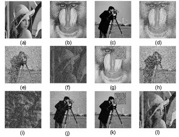
Sandra Nabil, Raffaella Balzarini, Frederic Devernay, James Crowley 189 P1.5 The Effects of Noise on Deep Learning Architectures
James Hamm, Thomas J. Naughton 193
P2.1 Feature Selection, Reduction and Classifiers using Histogram of Oriented Gradients: How important is Feature selection?
Ryan Melaugh, Nazmul Siddique, Sonya Coleman, Pratheepan Yogarajah 197
P2.2 Evaluation of Residual Learning in Lightweight Deep Networks for Object Classification
Arindam Das, Senthil Yogamani 205
P2.3 Comparison of Texture Recognition Algorithms
Christina Sherly, Sonya Coleman, Dermot Kerr, Bryan Gardiner, Chengdong Wu 209 P2.4 Vehicle Blind Spot Monitoring using YOLO Object Detection
Seam carving for content-aware wide-angle projection of panoramic
photography
Darren Coughlan and Paul Cuffe
School of Electrical Electronic Engineering, University College Dublin
Abstract
This paper presents a new method for the wide-angle projection of panoramic photographic imagery. The proposed methodology uses seam-carving techniques to improve the conformality of an equal-area projection of an image. Fundamentally, any wide-angle projection from a omnidirectional scene will contain distortion, however the aim of this method is to strategically introduce this distortion in areas of low salience in the image, to better preserve the appearance of the important content.
Keywords:Seam carving, omidirectional photography, wide-angle projection, panoramic photography
1
Introduction
In recent years there has been an increase in the use of omnidirectional cameras. With these devices and their associated stitching/montage software, it is possible to capture the entire scene around the camera, allowing the viewer to see 360◦horizontally by 180◦vertically [Scaramuzza, 2014]. By contrast, traditional wide angle cameras have a limited angle of view in the range of about 60◦to 80◦from centre. This paper proposes a new method to project a very wide-angle section of a captured spherical image to a flat plane. A field-of-view in the range of natural human vision is the goal here: up to perhaps 180◦horizontally by 120◦vertically.
The problem of representing a curved surface in a planar form is an ancient and well-documented area of research, due to its central relevance in cartography [Snyder, 1987]. All projections of the sphere contain some form of distortion in either area, conformality or interruption [Gauss, 1828] and cartographers must rou-tinely make compromises between these [Van Wijk, 2008]. Likewise, for panoramic photographic images, any projection to a flat plane will necessarily result in distortion of either shape or size.
There are various extant approaches to this problem of wide-angle projection. For instance, the method of [Zelnik-Manor et al., 2005] improves the appearance of wide angle panoramas by the use of multi-plane projec-tion. This method is not content-aware, and sharp distortion is noticeable if the edge of a projection plane passes through an area of importance in the image. In a similar way, the Panini projection [Sharpless et al., 2010] uses a fully three-dimensional scene, generated by a linear projection through the centre of the sphere. The image then shows a perspective view of part of the scene, allowing very wide-angle images to be created, up to 170◦. It is especially suited to architectural subject matter.
The primary contribution of this paper is in achieving similar results to those above using seam-carving [Avidan and Shamir, 2007] techniques, whereby no user interaction is required. The raw equirectangular output from the camera is first mapped to an equal-area projection, whereby objects in the planar image are congruent to their size in the panoramic sphere. Altering the dimensions of such an equal-area image to achieve confor-malitywithoutcontent-awareness would simply result in a classic projection like the Mercator, whereby salient objects in the image would no longer be equal-area (the island of Greenland is a well-known example from car-tograpy). Instead, the present technique seeks to achievelocal conformalityin areas of visual importance, with distortion moved to areas of less significance. The proposed method achieves this by incrementally introducing seams of low energy pixels into an equal-area projection, with the lengths of these seams chosen to restore the image’s conformality.
2
Methodology
The proposed technique has two stages: first, the raw output of the camera is projected to an equal-area format. Then, a section of the equal-area projection has seams inserted to restore its conformality in a content-aware way.
2.1
Equal-area projection
Before conformality can be restored, the raw image should first be projected to an area-preserving form.
2.1.1 Equirectangular
The equirectangular projection is important for panoramic imagery since it is typically the raw output format from omnidirectional cameras. The equirectangular projection is neither equal area or conformal: it projects the spherical image to a cylinder, and then unrolls this cylinder to a flat plane. The equations describing this projection are quite simple, as thex andy coordinates are direct mappings from the lines of longitude
λ and latitude φ, respectively. This simple mapping is why the equirectangular image format is used for omnidirectional photography.
x=(λ−λ0)cosφ1 (1)
y=(φ−φ1) (2)
Whereλ0andφ1are the central meridians in the spherical projection. Hence the equirectangular projection has coordinates from -180◦to 180◦in thex-axis and -90◦to 90◦in they-axis
2.1.2 Sinusoidal
The sinusoidal projection is a pseudocylindrical equal-area projection. There are several other equal-area pro-jections which would also be suitable as a starting point for manipulation, such as theMollweideor theBoggs eumorphic. The sinusoidal equal-area projection is chosen here due to its simplistic construction equations, which are below:
x=(λ−λ0)cosφ (3)
y=φ (4)
2.2
Content aware restoration of conformality
2.2.1 Graph creation
Seam carving adjusts image dimensions in a content-aware way by adding or removing low energy seams of pixels, found using shortest path algorithms on an appropriately-weighted graph [Avidan and Shamir, 2007].
The raster image of the sinusodial projection is transformed to a graphG whereby each node in the graph represents a pixel in the image. Each node in this network is then assigned six different attributes:
1. xandy-locations of the pixel in the original equirectangular image 2. Red, green and blues channel values
3. Greyscale luminosity
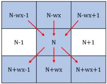
The graph is constructed to have directed edges in a six-connected format, to allow the seam calculation to be performed using shortest path algorithms. This connectivity is shown in fig. 1: each node has six connected edges, three incoming, and three outgoing. These edges are weighted by the absolute value of the difference in their luminosity value as in equation 5 which denotes the weight of the edge connecting nodesi andj.
W(ei→j)= |iLU M−jLU M| (5)
[image:13.595.331.506.421.558.2]This weighting is imposed so that when shortest paths through the graph are calculated, they will tend not to cross over edges in the image. This causes the shortest path calculation to act like an edge-detector would, avoiding visually salient content, and so this important content will tend to maintain the equal-area characteristic achieved with the initial sinusoidal projection.
Figure 1: Connective structure of nodes, numbered as though in a 3×3 image (w x = width of image = 3) When calculating the paths of lowest energy it is
important that each seam contains exactly one node from each row, such that the rows will increase in width by one pixel when seams are duplicated in the image. For this reason, the edges are directed to en-sure seams do not travel back up through the image and no edges exist between adjacent pixels to ensure a downward calculation of seam connectivity, as in fig. 1.
The manipulation in the top and bottom of the image will be opposite since the meridians are sinu-soidal curves which need to be straightened. There-fore, the initial graph G is split into two separate graphs Gt op and Gbot t om. The directed edges in Gbot t om are reversed for calculation of seams in the opposite direction (i.e up towards the equator) The
algorithm is symmetrically applied to each hemisphere in turn.
2.2.2 Seam carving methodology
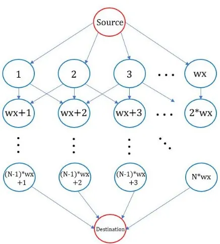
Figure 2: Subgraph connectivity, showing the node numbering scheme. A shortest path calculated from SourcetoDestinationis equivalent to finding the shortest path fromanynode in the top row toanynode in the bottom row
With φ+ as the upper vertical field of view, the number of pixels required to pad the top row inGt op isN =w x−cos(φ+)w x wherew x is the horizontal pixel resolution at the equator. Therefore, N seams will be introduced, all starting at the top row,φ+, but terminating at lower latitudes such that each row has the appropriate amount of padding pixels introduced i.e∝cos(φ)
To calculate these shortest path seams in Gt op, an appropriate loop creates a new subgraph on each iteration. In order to calculate the shortest path seam from top to bottom of these subgraphs, two additional nodes must be added as a source and destination. The source node is connected with directed edges of equal weight to each node in the top row of pixels, and the destination node is connected to each of the bottom row of pixels with directed edges of equal weight. This structure can be seen in fig. 2.
Once this shortest path has been calculated, the source and destination nodes are removed from the seam, and the seam is duplicated and inserted one position to the left, shifting the existing pixels to the right. This process is repeated for each row, to create a shifted image of more conformal dimensions.
This process is repeated for Gbot t om in an
in-verted format such that the source node is connected to the bottom row of nodes and destination node is connected to the top row of nodes. This therefore creates a bottom image which is also adjusted to confor-mal dimensions.
These images are then connected and adjusted such that each row of pixels is centred in the image. This creates a spatially varying conformal and equal-area projection of the wide angle image.
3
Implementation
The methodology was implemented in Python using the OpenCV library [Bradski, 2000] for image processing and NetworkX [Hagberg et al., 2008] for graph manipulation. The G.Projector [Schmunk, 2017] tool was used to create the sinusoidal projection. Omnidirectional photographs were captured using an LG 360 CAM (R105), for an image resolution of 5660×2830 pixels.
4
Results
4.1
Example processing steps
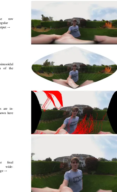
(a) The raw equirectangular camera output→
(b) The sinusoidal projection of the scene→
(c) Seams are in-serted, shown here in red→
[image:15.595.106.485.99.717.2](d) The final cropped wide-angle image→
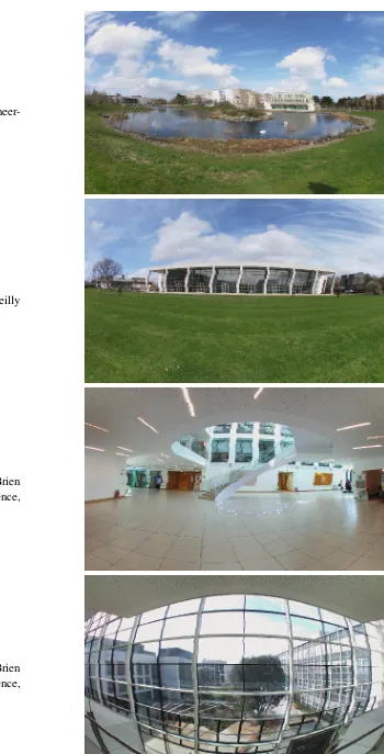
(a) UCD Engineer-ing BuildEngineer-ing
(b) UCD O’Reilly Hall
(c) UCD O’Brien Centre for Science, downstairs
[image:16.595.130.480.74.761.2]straightened image in fig. 3 (c) flares out in an hourglass shape. A cropped subimage to compensate for this effect is shown in fig. 3 (d), where the seams are not shown in red but instead using colours duplicated from adjacent pixels.
The final output of the algorithm, in fig. 3 (d) still contains some points of distortion, however it can be seen that aspects of the image such as the hedgerow appear more straightened. The roof of the house still shows some barrel distortion. This is where approaches such as that of [Sharpless et al., 2010] could perhaps be useful, as the user could draw straight lines on the image to be preserved. At the base of the image, the operator’s hand is also visible in a stretched and distracting form, however this is an artifact of the capture and stitching process, and is beyond the scope of the present discussion.
4.2
Other example images
Four other example images demonstrating the algorithm are shown in fig. 4. As a qualitative summary, the most successful image is perhaps fig. 4 (a) where an attractive wide angle view of a lake is presented. By contrast, fig. 4 (b) shows a weakness of the algorithm: the vertical columns appear jagged due to the irregular way that the seams are introduced. The seams are calculated based on a simple shortest path through the weighted graph: an improved technique might instead introduce seams with the explicit goal of maintaining the straightness and conformality of edges in the image. Similar artefacts can be perceived in fig. 4 (c) & (d). These images also show quite noticeable barrel distortion,
5
Conclusions & Future Work
New methods have been described to improve the presentation of wide angle images through the use of seam carving techniques. The results indicate that the seam carving holds promise for the wide angle projection of photographic imagery. However, more sophisticated objectives for inserting seams, such as the enhance the rectilinearity of salient image features, seem necessary if projection free of noticeable distortion is to be achieved.
References
[Avidan and Shamir, 2007] Avidan, S. and Shamir, A. (2007). Seam carving for content-aware image resizing. InACM Transactions on graphics (TOG), volume 26, page 10. ACM.
[Bradski, 2000] Bradski, G. (2000). The OpenCV Library.Dr. Dobb’s Journal of Software Tools.
[Carroll et al., 2009] Carroll, R., Agrawala, M., and Agarwala, A. (2009). Optimizing content-preserving projections for wide-angle images. ACM Trans. Graph., 28(3):43–1.
[Gauss, 1828] Gauss, C. F. (1828). Disquisitiones generales circa superficies curvas, volume 1. Typis Di-eterichianis.
[Hagberg et al., 2008] Hagberg, A., Swart, P., and S Chult, D. (2008). Exploring network structure, dynamics, and function using networkx. Technical report, Los Alamos National Lab.(LANL), Los Alamos, NM (United States).
[Scaramuzza, 2014] Scaramuzza, D. (2014). Omnidirectional Camera, pages 552–560. Springer US, Boston, MA.
[Sharpless et al., 2010] Sharpless, T. K., Postle, B., and German, D. M. (2010). Pannini: a new projection for rendering wide angle perspective images. InProceedings of the Sixth international conference on Compu-tational Aesthetics in Graphics, Visualization and Imaging, pages 9–16. Eurographics Association.
[Snyder, 1987] Snyder, J. P. (1987). Map projections–A working manual, volume 1395. US Government Printing Office.
[Van Wijk, 2008] Van Wijk, J. J. (2008). Unfolding the earth: myriahedral projections. The Cartographic Journal, 45(1):32–42.
[Zelnik-Manor et al., 2005] Zelnik-Manor, L., Peters, G., and Perona, P. (2005). Squaring the circle in panora-mas. In Computer Vision, 2005. ICCV 2005. Tenth IEEE International Conference on, volume 2, pages 1292–1299. IEEE.
[Zhu et al., 2011] Zhu, T., Wang, W., Xie, Y., and Heng, P.-A. (2011). An ellipsoid-based perspective projec-tion correcprojec-tion for wide-angle images. InSIGGRAPH Asia 2011 Posters, page 43. ACM.
Colour Correction for Stereoscopic Omnidirectional Images
1
Simone Croci,
1Mairead Grogan,
1,2Sebastian Knorr,
1Aljosa Smolic
1
V-SENSE Project, School of Computer Science and Statistics, Trinity College Dublin;
2
Communication Systems Group, Technical University of Berlin
Spherical Voronoi Diagram
Highlighted Colour Mismatch in left ERP Image S3D Image with overlaid Voronoi
Diagram in ERP Format Colour Corrected S3D Image in ERP Format X
Y Z
Highlighted Colour Mismatch in left ERP Image
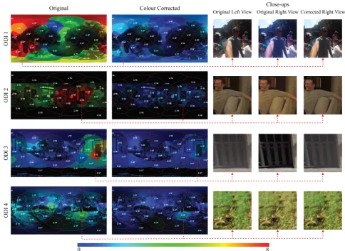
Figure 1: Colour mismatch correction and detection based on the spherical Voronoi diagram.
Abstract
Stereoscopic omnidirectional images (ODI) when viewed with a head-mounted display are a way to gen-erate an immersive experience. Unfortunately, their creation is not an easy process, and different problems can be present in the ODI that can reduce the quality of experience. A common problem is colour mismatch, which occurs when the colours of the objects in the scene are different between the two stereoscopic views. In this paper we propose a novel method for the correction of colour mismatch based on the subdivision of ODIs into patches, where local colour correction transformations are fitted and then globally combined. The results presented in the paper show that the proposed method is able to reduce the colour mismatch in stereoscopic ODIs.
Keywords:Virtual reality, 360-video, colour matching, binocular rivalry, stereoscopic 3D
1
Introduction
One of the most popular formats to deliver virtual reality experiences is 360-video which is often referred to as VR-video or cinematic VR. Shooting 360-video is a technological challenge as there are many technical limitations which need to be overcome, especially for capturing and post-processing in stereoscopic 3D (S3D). 360-video is often captured with an omnidirectional multi-camera rig and stitched together in post-production [Zhang and Liu, 2015]. In general, the limitations inherent in 360 videos result in artifacts which cause visual discomfort when watching the content with a head-mounted display. The artifacts or issues can be divided into three categories: binocular rivalry issues (e.g. colour mismatch), conflicts of depth cues (e.g. vergence-accomodation conflicts), and artifacts which occur in both monocular and stereoscopic 360-degree content production (e.g. stitching artifacts) [Knorr et al., 2017].
Figure 2: Overall system for colour mismatch correction and detection.
of multiple views into a single monocular panorama, but also between the left and right view of a stereoscopic panorama, which often result in visual discomfort [Knorr et al., 2012].
In this context, we introduce a novel approach and entire system for colour mismatch correction and detec-tion in S3D omnidirecdetec-tional content. The system consists of three main modules: pre-processing, local colour correction between the left and right stereoscopic ODIs, and colour mismatch detection as shown in Figure 2. During the pre-processing step, we compute a spherical Voronoi diagram and extract Voronoi patches in the equirectangular projection (ERP) format of the left and right ODI. Then, we estimate pixel correspondences between the corresponding patches in both views and apply a local colour transfer in order to match the colours of the corresponding patches, which is the main contribution of this paper. Finally, our patch-based colour mismatch detection module [Croci et al., 2017] measures and visualises colour mismatch, which might still be present, between the left and right stereoscopic ODIs. While the entire colour correction approach is applied in the RGB colour space and uses a colour transfer approach introduced in [Grogan and Dahyot, 2017], the colour mismatch detection module is applied in the Lab colour space and uses colour statistics analysis proposed in [Reinhard et al., 2001]. This allows a more objective and independent evaluation of still existing colour discrep-ancies between the views. Finally, we evaluate the entire system on 15 S3D ODIs with large colour mismatch and show that our system improves the quality of the ODIs significantly.
The remainder of the paper is organised as follows. In Section 2, related work in artifact detection and colour correction is reviewed. Then, in Section 3, we describe the proposed system for the subdivision of the ODI into patches, the colour correction step, and the colour mismatch detection. In Section 4, the proposed colour correction method is evaluated with 15 S3D ODIs. Finally, in Section 5, the paper concludes with a discussion and future work.
2
Related Work
Colour mismatch detection and colour correction in stereoscopic and multi-view applications has been an ongo-ing research topic for many years. In [Dong et al., 2013], a method for detectongo-ing stereo camera distortions based on statistical models was presented in order to evaluate vertical misalignment, camera rotation, unsynchronised zooming, and colour mismatch in S3D content.
A large variety of artifact detection methods, including a method for the detection of colour mismatch, was introduced in [Voronov et al., 2013]. More recently, in [Knorr et al., 2017, Croci et al., 2017], S3D quality assessment methods for stereoscopic ODIs were introduced which also focus on colour mismatch detection.
In the computer vision and multi-view video processing communities, the initial efforts on solving colour mismatches between multiple views used exposure compensation (or gain compensation) [Xu and Mulligan, 2010]. This approach adjusts the gain level of images to compensate for appearance differences caused by different exposure levels. However, this approach may fail in the case of local differences e.g. caused by lens flares or polarization.
stereo-X
Y Z
αi di
Pi r
Zi VCi
ΩS
(a) Spherical Voronoi diagram.
extended search region (left image)
VCi VC
bounding box
extended search region (right image)
L
i R
(b) Disparity compensation.
Figure 3: Spherical Voronoi diagram and disparity compensation.
scopic image pairs. The algorithm uses dense stereo matching and global colour correction to initialise colour values, and then improves the local colour smoothness and global colour consistency of the resulting image.
For large baseline multi-view video, [Ye et al., 2017] introduced a robust colour correction method that en-forces spatio-temporal colour consistencies and gradient preservation by solving a global optimization problem. The authors of [Xia et al., 2017] proposed an effective colour correction method for multi-view image stitching which first finds coherent content regions in inter-image overlaps, and then parameterise a colour remapping curve as transform model.
The image processing and computer graphics communities were developing similar colour manipulation methods, calledcolour transfer techniques. These methods transfer the colour feel from a palette image to a target image, and assume that the content of the images is different. The earliest work in this area was by [Reinhard et al., 2001], who proposed transforming the mean and standard deviation of each colour channel in the target image to match that of the palette image. Since then, more complex techniques have been used to model the colour distributions of the images more accurately, including histograms and Gaussian Mixture models [Pitie et al., 2005, Tai et al., 2005]. While global colour transfer functions are often used, including affine, radial basis and optimal transport functions [Pitié and Kokaram, 2007, Grogan et al., 2017, Bonneel et al., 2016], local techniques have also been proposed to allow for more flexibility in the recolouring [Wang et al., 2010, Shih et al., 2013]. Recently, Grogan and Dahyot [Grogan and Dahyot, 2017, Grogan et al., 2015] proposed a colour transfer technique that could also be enhanced to take into account colour correspondences between the target and palette images, ensuring the method could be used to colour correct images of the same scene. They showed that this method performed as well as other state of the art colour corrections techniques, with the advantage of being more robust to correspondence outliers. In this paper, we extend this method so that it can be used to successfully colour correct stereoscopic ODIs.
3
Proposed Method
The complete system for the correction and detection of colour mismatch is illustrated in Figure 2. Its three main components, that is, the pre-processing step, the local colour correction, and the colour mismatch detection are described in the next sections.
3.1
Pre-processing Step
αi=(i−1)π·¡3− p
5¢
,Zi=¡1−n1¢· ³
1−2(in−−11) ´
,di= q
1−Zi2,Xi=di·cos(αi)andYi=di·si n(αi), whereαi is the azimuthal angle anddi is the distance of the point from the z-axis. From then evenly distributed points, the spherical Voronoi diagram basically partitions the surface of the sphereΩS into n cellsV Ci, where each point in the cellV Ci is closer to the corresponding pointPi than to any of the other evenly distributed points Pj. Formally, the cellV Ci is defined as follows:
V Ci={P∈ΩS|dS(P,Pi)≤dS(P,Pj)∀j6=i}, (1)
wheredS(P,Pi) is the spherical distance between the current pointPand the pointPi, i.e., the length of the shortest path on the surface of the sphere connecting these two points.
Next, we map each cellV Ci of the spherical Voronoi diagram to a planar image patchΠi. For each cell, a planar patch is positioned on the centroid of the cell, tangent to the sphere. The points on the sphere and the planar patch are related by central projection, and the pixel values of the patch are computed by sampling the ODI in ERP format using bilinear interpolation. The resolution of each patch is defined by the pixels per visual angle, a parameter that is kept constant for each patch. In the presence of disparity, it can occur that a region inside a Voronoi cell in one view is outside the same cell in the other view. In order to cope with the disparity, we add a border around the Voronoi cell when the patch is extracted, as shown in Figure 3b.
The number of patches and thus the size of each patch influences the reduction of the colour mismatch. If the colour mismatch is localised in a small region and the patch is large, then the proposed method could have difficulty in matching the colours between the two views. We have empirically found that 30 patches is a good number for most of the ODIs that we have processed.
3.2
Local Colour Correction
The local colour correction component of the system involves first estimating colour correspondences {cL(k),cR(k)}k=1..m between corresponding patches of the left and right view. We investigated two methods for the estimation of correspondences: the Semi-Global Block Matching approach [Hirschmuller, 2008] and the Coarse-to-Fine PatchMatch approach [Hu et al., 2016], but we found no significant difference between the colour correction results generated using these approaches.
For each patch, we use the correspondences to estimate a colour transformation which recolours the patch of the right view so that it is more similar to the left, using the method proposed in [Grogan and Dahyot, 2017]. For each patch, we fit two Gaussian Mixture modelsG M ML andG M MR to the left and right colour correspondences respectively:
G M MY(x)= 1 m
m X
k=1
N(x;cY(k),hI), withY ∈{L,R}, (2)
wherex∈R3are colour values of the RGB colour space, and each GaussianN is associated with an identical isotropic covariance matrix,hI. The goal is to align the two Gaussian Mixture models by warping the right one as follows:
G M MR0(x|θ)= 1 m
m X k=1
N(x;φ(cR(k),θ),hI), (3)
whereφrepresents a parametric Thin Plate Spline (TPS) transformation controlled by the parameterθ. Tech-nically, the alignment beteweenG M ML and the warpedG M MR0 is obtained by minimising the L2 distance between them. ThisL2technique has been shown to be robust to correspondence outliers, and the smooth TPS function ensures that similar colours in the patch remain similar after recolouring, eliminating artifacts in the gradient of the image which can appear when using other recolouring methods [Pitie et al., 2005].
contributions of each of the transformations when recolouring the ODI. To compute the value of a pixel in the weight maskGi, the spherical distance between this pixel in the spherical ODI and the centroid of the Voronoi cellV Ci is computed, and a Gaussian function is applied to it. In this way, inGi, pixels that lie close to the centroid in the ODI will have higher weights than those further away. Then, when recolouring the ODI of the right viewIR in ERP format to its corrected versionIˆR, the colour of the pixel at location(j,k)is given by:
ˆ
IR(j,k)= Pn
i=1Gi(j,k)·φi(IR(j,k),θ) Pn
i=1Gi(j,k)
. (4)
In this manner, each local colour transformation has the most influence in the area from which it is estimated, and the colour transformations are smoothly blended without creating any artifacts at the patch borders.
3.3
Colour Mismatch Detection
The colour mismatch detection applied after the colour correction of the ODI, and useful for getting feedback on the remaining colour mismatch, is a simplification of the colour mismatch detection proposed in [Croci et al., 2017]. The simplification is obtained by discarding the saliency, since it is not available for all the 15 ODIs processed in this paper. As mentioned in Section 3.1, the detection module also uses Voronoi patches for colour mismatch detection and localization. First, the ODI is partitioned into patches. Then, correspondences are computed for corresponding patches between the two views using the Semi-Global Block Matching approach introduced in [Hirschmuller, 2008]. The correspondences are necessary in order to identify the regions that are present in both views of the patch. From the common regions, the colour meansµL andµR, and the colour standard deviationsσL andσR are estimated in the Lab colour space as proposed in [Reinhard et al., 2001]. Finally, for each patchΠi the following colour mismatch score is computed:
C M Si= q
° °µL−µR
° ° 2
+λkσL−σRk2, (5)
whereλis a tuning parameter that was set to one for the analysis of the ODIs. The patch scores can be visualised with the jet colourmap and overlaid with the ODI in ERP format as shown in the teaser in Figure 1. In order to get the global scoreC M Sg l obal for the entire ODI, the patch scores are simply averaged:
C M Sg l obal= Pn
i=1C M Si
n . (6)
4
Results
In order to evaluate the proposed method, we selected 14 ODIs with the highest colour mismatch scores from the dataset introduced in [Croci et al., 2018], and one ODI which was captured with a 360◦mirror-rig. Figure 4a shows a bar chart with the global colour mismatch scores computed with Equation 6 before and after applying the proposed colour correction method. In this figure, one can see that the novel approach is able to reduce the colour mismatch in all ODIs by an average of 74%. The largest score reduction, equal to 89%, was observed for ODI 1.
Figure 4b shows for four ODIs the individual colour mismatch patch scores and their visualisation using the jet colourmap before and after colour correction, together with some close-ups. ODI 1 is a clear example of strong colour mismatch where our method is able to significantly reduce it, as can be clearly seen in the close-up. ODI 2 and ODI 3 also show a strong colour mismatch localised to a particular region. Even in these two cases, our method fixes the mismatch. For ODI 4, the close-up shows how even minor colour mismatches can be corrected.
(a) Global colour mismatch scores before and after colour correction (used camera rigs are specified in brackets).
[image:24.595.54.539.334.687.2](b) Sample ODIs with colour mismatch visualisation (red: strong mismatch, blue: no mismatch) and close-ups before and after colour correction.
5
Conclusions
This paper presented a solution to the problem of colour mismatch in stereoscopic ODIs, which can cause visual discomfort. The proposed approach first divides the ODI into patches using the spherical Voronoi diagram from evenly distributed points on the sphere. In each patch a colour transformation is fitted from correspondences in the RGB colour space, and then the colour transformations are combined together using weight masks based on the spherical distance from the centroid of the Voronoi cells. In order to analyse colour mismatch objectively and independently, the processed ODI is analysed in the Lab colour space using an alternative correspondence estimation approach.
The results show that the proposed approach is able to reduce the colour mismatch significantly. This conclusion was obtained by computing the global and local patch colour mismatch scores before and after ap-plying the colour correction approach on different ODIs. In particular, 89% is the largest global score reduction that was observed. However, the proposed method is not exempt from limitations related to the accuracy of the correspondence estimation, and the misalignment of the patches with the region characterized by colour mismatch.
In the future, we plan to improve the proposed approach by tackling some of the limitations, especially the misalignment of the patch with the region affected by colour mismatch. The plan is to investigate the possibility to have adaptable patches to the region with colour mismatch.
Acknowledgments
This publication has emanated from research conducted with the financial support of Science Foundation Ire-land (SFI) under the Grant Number 15/RP/2776.
References
[Aurenhammer, 1991] Aurenhammer, F. (1991). Voronoi Diagrams - A Survey of a Fundamental Data Struc-ture.ACM Comput. Surv., 23(3):345–405.
[Bonneel et al., 2016] Bonneel, N., Peyré, G., and Cuturi, M. (2016). Wasserstein barycentric coordinates: Histogram regression using optimal transport. ACM Trans. Graph., 35(4):71:1–71:10.
[Croci et al., 2017] Croci, S., Knorr, S., Goldmann, L., and Smolic, A. (2017). A framework for quality control in cinematic VR based on Voronoi patches and saliency. InIEEE Int. Conf. 3D Immersion (IC3D), Brussels, Belgium.
[Croci et al., 2018] Croci, S., Knorr, S., and Smolic, A. (2018). Sharpness mismatch detection in stereoscopic content with 360-degree capability. IEEE Int. Conf. Image Processing (ICIP).
[Dong et al., 2013] Dong, Q., Zhou, T., Guo, Z., and Xiao, J. (2013). A stereo camera distortion detecting method for 3DTV video quality assessment. InIEEE Asia-Pacific Signal and Inform. Process. Assoc. Annu. Summit and Conf., pages 1–4.
[Grogan and Dahyot, 2017] Grogan, M. and Dahyot, R. (2017). Robust registration of Gaussian mixtures for colour transfer. CoRR, abs/1705.06091.
[Grogan et al., 2017] Grogan, M., Dahyot, R., and Smolic, A. (2017). User interaction for image recolouring using L2. InProc. of the 14th European Conf. on Visual Media Prod., CVMP 2017, pages 6:1–6:10, New York, NY, USA. ACM.
[Hirschmuller, 2008] Hirschmuller, H. (2008). Stereo processing by semiglobal matching and mutual infor-mation.IEEE Trans. Pattern Anal. Mach. Intell., 30(2):328–341.
[Hu et al., 2016] Hu, Y., Song, R., and Li, Y. (2016). Efficient coarse-to-fine patch match for large displacement optical flow. InIEEE Conf. on Comput. Vision and Pattern Recognition (CVPR), pages 5704–5712.
[Knorr et al., 2017] Knorr, S., Croci, S., and Smolic, A. (2017). A modular scheme for artifact detection in stereoscopic omni-directional images. InProc. of the Irish Mach. Vision and Image Process. Conf. (IMVIP).
[Knorr et al., 2012] Knorr, S., Ide, K., Kunter, M., and Sikora, T. (2012). The avoidance of visual discomfort and basic rules for producing "good 3D" pictures. SMPTE Motion Imaging J., 121(7):72–79.
[Pitié and Kokaram, 2007] Pitié, F. and Kokaram, A. (2007). The linear monge-kantorovitch linear colour mapping for example-based colour transfer. InVisual Media Prod., 2007. IETCVMP. 4th European Conf. on, pages 1–9.
[Pitie et al., 2005] Pitie, F., Kokaram, A., and Dahyot, R. (2005). N-dimensional probability density function transfer and its application to color transfer. InIEEE Int. Conf. Comput. Vision (ICCV), volume 2, pages 1434–1439 Vol. 2.
[Reinhard et al., 2001] Reinhard, E., Ashikhmin, M., Gooch, B., and Shirley, P. (2001). Color transfer between images. IEEE Comput. Graph. Appl., 21(5):34–41.
[Shih et al., 2013] Shih, Y., Paris, S., Durand, F., and Freeman, W. T. (2013). Data-driven hallucination of different times of day from a single outdoor photo. ACM Trans. Graph., 32(6):200:1–200:11.
[Tai et al., 2005] Tai, Y.-W., Jia, J., and Tang, C.-K. (2005). Local color transfer via probabilistic segmentation by expectation-maximization. InIEEE Conf. on Comput. Vision and Pattern Recognition (CVPR), volume 1, pages 747–754 vol. 1.
[Voronov et al., 2013] Voronov, A., Vatolin, D., Sumin, D., Napadovsky, V., and Borisov, A. (2013). Method-ology for stereoscopic motion-picture quality assessment. InProc. of the SPIE, Stereoscopic Displays and Appl. XXIV, volume 8648.
[Wang et al., 2010] Wang, B., Yu, Y., Wong, T.-T., Chen, C., and Xu, Y.-Q. (2010). Data-driven image color theme enhancement.ACM Trans. Graph., 29(6):146:1–146:10.
[Wang et al., 2011] Wang, Q., Yan, P., Yuan, Y., and Li, X. (2011). Robust color correction in stereo vision. In Int. Conf. Image Processing (ICIP), number 2, pages 965–968.
[Xia et al., 2017] Xia, M., Yao, J., Xie, R., and Zhang, M. (2017). Color Consistency Correction Based on Remapping Optimization for Image Stitching. InIEEE Int. Conf. Comput. Vision (ICCV).
[Xu and Mulligan, 2010] Xu, W. and Mulligan, J. (2010). Performance evaluation of color correction ap-proaches for automatic multi-view image and video stitching. InIEEE Conf. on Comput. Vision and Pattern Recognition (CVPR), pages 263–270.
[Ye et al., 2017] Ye, S., Lu, S. P., and Munteanu, A. (2017). Color correction for large-baseline multiview video. Elsevier Signal Process.: Image Commun., 53(January):40–50.
[Zhang and Liu, 2015] Zhang, F. and Liu, F. (2015). Casual stereoscopic panorama stitching. InIEEE Conf. on Comput. Vision and Pattern Recognition (CVPR), pages 2002–2010.
Artifacts reduction in JPEG-Compressed Images using CNNs
Fatma Albluwi, Vladimir A. Krylov & Rozenn Dahyot
School of Computer Science and Statistics, Trinity College Dublin, Ireland
Abstract
The most popular MPEG and JPEG image compression formats can produce a combination of distorting effects in images such as blurring, ringing and blocking artifacts. We propose an approach that mitigates this undesirable compression drawback based on the use of convolutional neural networks (CNNs). Our solution enhances the visual quality of decompressed images by automatically correcting any such artifacts. We also show experimentally that our proposed CNN architectures can give the same or better results compared to the existing deeper architectures that are more costly computationally.
Keywords:JPEG Compression Artifacts, Image Enhancement, Convolutional Neural Networks,
Deblock-ing, Deblurring.
1
Introduction
It has become commonplace to apply lossy compression, e.g., JPEG and HEVC-MSP, to images and videos to save storage space and bandwidth. A lot of attention has been attracted to enhancing the quality and com-pression power of algorithms, in particular, in large companies operating huge image and video volumes like Facebook and Twitter. Compression is a family of data encoding techniques that often rely on inexact approx-imations to represent the encoded content in order to achieve the most competitive performance. This leads to undesirable artifacts such as blurring, blocking and ringing, which are addressed by artifact reduction methods. JPEG compression is probably the widest used lossy image compression approach. The underlying tech-nique separates an image into8×8pixel-blocks followed by the Discrete Cosine Transformation (DCT) ap-plied to each block separately. In order to achieve compression, the quantization is then performed on the DCT coefficients, which inevitably results in the appearance of visual artifacts. Blurringappears because the high-frequency components are lost.Ringing, also referred to as theGibbs phenomenon, takes place because of the coarse quantization of the high-frequency components. Finally, theblockingartifacts are due to the separate processing and encoding of blocks without consideration and, hence, loss of adjacency information between the blocks.
There are many different methods that have been proposed in the literature to deal with the different types of artifacts, some of which targeting specific types of compression side-effects. For example,
de-blocking methods are utilized to decrease the blocking artifacts by applying filters on or across the borders
[Reeve and Lim, 1984, Nosratinia, 1999, List et al., 2003, Wang et al., 2013], or using thresholding by wavelet transform [Liew and Yan, 2004] or by Shape-Adaptive DCT transform (SA-DCT) [Foi et al., 2007]. Although these methods deal reasonably well with blocking artifacts and ringing effects, the results suffer from blurring. Other methods consider compression as distortion which requires reconstruction techniques [Yang et al., 1995, Sun and Cham, 2007, Jung et al., 2012, Jancsary et al., 2012]. These methods output sharpened images featur-ing smooth regions and noisy edges. More recently, deep convolutional neural networks (CNNs) have been used to mitigate the compression artifacts and restore the distorted images [Dong et al., 2015, Svoboda et al., 2016a] delivering state-of-the-art results.
more efficiently. Firstly, we present a novel CNN (referred to as SA-CAR6) for image restoration which deliv-ers better performance than the state-of-the-art CNN-based models [Dong et al., 2015, Svoboda et al., 2016a] and employs less parameters. Smaller models are a clearly better option since they reduces the computational complexity, and allow us to avoid problems of big networks such as overfitting, vanishing or exploding gradi-ents, etc. Secondly, we consider several CNNs with different parameter counts (CAR3, CAR4, DA-CAR5) to show that we can get the same or better results using smaller networks with a lower parameter count.
2
Related Work
A variety of methods have been proposed to reduce the artifacts in JPEG compressed images. These can gen-erally be divided into two main types: deblocking methods and restoration methods. The deblocking meth-ods are focused on suppressing ringing and blocking artifacts and various types of filters have been utilized in the spatial domain to remove the blocking artifacts [Reeve and Lim, 1984, Nosratinia, 1999, List et al., 2003, Wang et al., 2013]. Wavelet transform has also been employed to perform denoising in the frequency do-main [Liew and Yan, 2004]. One of the most recent state-of-the-art deblocking methods is the Pointwise Shape-Adaptive DCT [Foi et al., 2007]. This approach, however, is not capable of reproducing sharp edges and it oversmoothes the image textures. On the other hand, restoration methods deal with the compression as dis-tortion operation which requires restoration, These methods include: projection on convex sets based method (POCS) [Yang et al., 1995], solving a MAP problem (FoE) [Sun and Cham, 2007], and sparse-coding-based methods [Jung et al., 2012]. The current state-of-the-art method is the Regression Tree Fields based method (RTF) [Jancsary et al., 2012].
Recently, convolutional neural networks (CNNs) [Goodfellow et al., 2016] have been successfully applied to reconstruct images corrupted by JPEG compression [Dong et al., 2015, Svoboda et al., 2016a], as well as to related image enhancement problems, such as super-resolution [Dong et al., 2014, Kim et al., 2016], mo-tion deblurring [Sun et al., 2015, Svoboda et al., 2016b], non-blind image deconvolumo-tion [Xu et al., 2014], text deblurring [Hradiš et al., 2015] and image denoising [Jain and Seung, 2009]. Dong et al. utilized the CNN to remove the compression artifacts (AR-CNN: Artifacts Removing using Convolutional Neural Network) [Dong et al., 2015]. The structure of AR-CNN depends on Super Resolution CNN (SRCNN) which was pro-posed to infer high resolution images from lower resolution input [Dong et al., 2014]. The SRCNN architecture consists of 3 layers: feature extraction layer, non-linear mapping layer, reconstruction layer, and this structure has been set according to the sparse coding method. The 3-layers SRCNN was not sufficient to restore com-pressed images, so extra feature enhancement layers were added to SRCNN after the feature extraction layer to enhance the extracted features, which resulted in a 4-layers AR-CNN.
Svoboda et al. proposed two different convolutional networks for JPEG restoration called L4 and L8 Resid-ual architectures [Svoboda et al., 2016a]. Similar to Kim et al. for super-resolution [Kim et al., 2016], resid-ual learning was adopted in L4 and L8, where the network learns the residresid-ual imager=x−ˆx. The estimated residual imageris then subtracted from the corrupted input xto get the restored output image ˆx, instead of learning the reconstructed whole image directly. Their approach is based on the idea of “deeper is better”, but deeper networks take a long time to train and may suffer from overfitting and vanishing or exploding gradients. To alleviate this problems, the skip architecture was employed [Long et al., 2015] as well as residual learn-ing [He et al., 2016]. The skip architecture allows the network “shortcut” the input to the intermediate layers. This allows the more complex image content to be used in the middle layers as the local context information, since is it critical for reducing the impact of artifacts.
3
Methodology
ReLU) [Maas et al., 2013]. In the absence of pooling and deconvolution layers, the filter size is the only factor that affects the output image size. Zero padding should be used to compensate for the size decrease if one wants the output of the same size.
3.1
Formulation
The first hidden layer (patch extraction and representation) extracts the overlapping patches from the input images and then represents each patch as a high-dimensional vector. The last layer, also called reconstruction layer, assembles the restored image by aggregating the patch-wise representations. The structure of a CNN is as follows:
F0(x)=x (1)
Fi(x)=max¡0,Wi∗Fi−1(x)+bi¢ i∈{1, 2, . . . ,L−1} (2)
F(x)=WL∗FL−1(x)+bL (3)
wherexis the compressed image andWi andbi are the filters and biases.Wi is comprised ofni filters which supportni−1×fi×fi;n0is the number of channels in the input image andfiis a filter size.Fi(x)are the feature maps in the layeri, andF(x)is the reconstructed output image which has the same size as the input image. Lis the number of convolutional layers in the architecture. The activation function type employed is Leaky ReLU.
3.2
Optimization
The filter weights in each layer are initialized by a robust initialization method proposed in [He et al., 2015] for ReLU. The aim is to recover images{F(xi)}from the corresponding JPEG-compressed{xi}that are as similar as possible to the set of ground truth images{yi}. The estimation ofΘ={W1,W2, . . . ,WL,b1,b2, . . . ,bL}is required to specify the end-to-end mapping functionF. The cost minimization between the reconstructed imagesF(x,Θ) and its original imagesyis applied. The MSE functionC(Θ)is employed as the training loss function:
C(Θ)= 1
n
n X i=1
||F(xi;Θ)−yi||2 (4)
The minimization is performed using using Adamax [Kingma and Ba, 2014], which is a technique to optimize CNNs at faster convergence rates.
3.3
CNN architecture and training
CNN can be shaped to different structures for deep learning problems such as the direct architecture (Fig. 1a) and skip architecture (Fig. 1b). In the direct architecture, the image is transfered successively through layers from the input layer to the output layer. This approach is used in many tasks of low-level image processing [Dong et al., 2014, Dong et al., 2015, Hradiš et al., 2015, Svoboda et al., 2016b], and it often results in high performance. On the other hand, a skip architecture interrupts the successive flow of data by allowing skip connections to merge layers that have undergone different processing paths. There are several main merger operations, such as concatenating, adding, subtracting, etc. The skip architecture may alleviate some specific problems of propagating information through deeper networks, such as, specifically, vanishing and exploding gradients [Long et al., 2015, He et al., 2016, Svoboda et al., 2016a].
JPEG-Compressed
image (Input) Reconstructed
image (Output)
Feature Extraction Reconstruction
. . .
(a) Direct Architecture
JPEG-Compressed
image (Input) Reconstructed image (Output)
Feature Extraction Concatenated layers Reconstruction
. . .
(b) Skip Architecture
Figure 1: Different structures of the CNN networks: direct and skip architectures.
For CNN architectures the training time is typically proportional to the size of training samples and the total parameter countWt ot al:
Wt ot al= L X i=1
ni−1×ni×fi2 (5)
The testing (inference) time efficiency is of critical importance for practical use and also increases with the number of parameters. Deep learning can efficiently process big data sizes for training and one of the ways to reduce overfitting, is by using a smaller network with fewer parameter. The advantage of smaller networks is overwhelming when they practically allow one to achieve the same or even higher performances on the same training dataset. In this work, we endeavour to do just that: propose smaller network architectures that perform better.
4
Experimental results
In Sec. 4.1 we present the dataset employed and in Sec. 4.2 the metrics used for evaluation and comparisons. Sec. 4.3 reports evaluation resulsts and comparisons with state-of-the-art models.
4.1
Data & training
The BSDS500 dataset [Arbelaez et al., 2011] contains 400 training images that were used for training all net-works, and 100 images we have employed to perform validation. LIVE1 dataset [Sheikh et al., 2005] is used as test set and it has 29 images often used for super-resolution [Yang et al., 2014] and image quality assessment [Wang et al., 2004]. The training images are split into33×33sub-images{yi}. These sub-images are generated from the ground truth images with a stride of 10, to create 521,984 sub-images. We have transformed the RGB images into YCbCr color model to deal with gray-scale by using the Y channel (luminance component). The network is trained on a batch size of 64. The JPEG-compressed images{xi}are generated from the gray-scale sub-images using MATLAB JPEG encoder. We have used two different quality settings: q = 10 (low qual-ity), and q = 20 (mild quality). The number of training epochs is set to 60. All implementations are in Keras (Python, TensorFlow backend), with training and experiments run on the following system: Intel(R) Core i7 CPU (2.80 GHz), 16GB RAM, GTX Geforce 1050 GPU.
4.2
Quantitative metrics for comparisons
Table 1: Average image reconstruction results reported by PSNR (dB), PSNR-B (dB) and SSIM on the LIVE1 dataset for JPEG quality q = 10 (best resultin bold, second best resultin italic).
Architecture Number
of Layers Filter size Feature maps PSNR PSNR-B SSIM
Parameter count
Input JPEG-decompressed - - - 27.77 25.33 0.791
-SA-DCT [Foi et al., 2007] - - - 28.65 28.01 0.809
-SRCNN [Dong et al., 2015] 3 (9-1-5) (64-32-1) 28.91 28.52 0.818 8,032 AR-CNN [Dong et al., 2015] 4 (9-7-1-5) (64-32-16-1) 28.98 28.70 0.822 106,448
DA-CAR3 3 (9-7-5) (64-32-1) 29.08 28.71 0.823 106,336
DA-CAR4 4 (9-3-3-5) (64-32-32-1) 29.07 28.71 0.823 33,632
DA-CAR5 5 (9-5-5-5-5) (32-32-32-32-1) 29.14 28.77 0.825 80,192
L4 Residual 4 (11-3-3-5) (48-64-64-1) 29.08 28.71 0.824 71,920 [Svoboda et al., 2016a]
SA-CAR6 6 (9-5-5-5- (32-32-32-32- 29.16 28.80 0.826 131,392
(2+1) 5-5) 32-1)
Table 2: Average image reconstruction results reported by PSNR (dB), PSNR-B (dB) and SSIM on the LIVE1 dataset for JPEG quality q = 20 (best resultin bold, second best resultin italic).
Architecture Number
of Layers Filter size Feature maps PSNR PSNR-B SSIM
Parameter count
Input JPEG-decompressed - - - 30.07 27.57 0.868
-SA-DCT [Foi et al., 2007] - - - 30.81 29.82 0.878
-AR-CNN [Dong et al., 2015] 4 (9-7-1-5) (64-32-16-1) 31.29 30.76 0.887 106,448 L4 Residual 4 (11-3-3-5) (48-64-64-1) 31.42 30.83 0.890 71,920 [Svoboda et al., 2016a]
L8 Residual 8 (11-3-3-3- (32-64-64-64- 31.51 30.92 0.891 220,064 [Svoboda et al., 2016a] (4+1),(6+1) 1-5-1-5) 64-64-128-1)
SA-CAR6 6 (9-5-5-5- (32-32-32-32- 31.52 30.97 0.892 131,392
(2+1) 5-5) 32-1)
4.3
Benchmark comparisons
AR-CNN [Dong et al., 2015] is based on feature enhancement and an extra layer was originally added after the feature extraction layer to further refine and enhance the features. Our DA-CAR3 architecture allows us to achieve the same performance by using only three layers when using suitable filter sizes (see Table 1). In practice, AR-CNN (9-7-1-5) is better than SRCNN (9-1-5) because of the larger filter size in the second layer of AR-CNN (9-7-1-5).
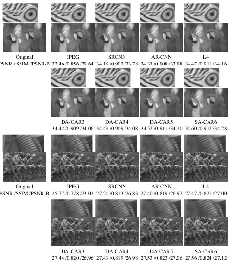
Original JPEG SRCNN AR-CNN L4
PSNR/SSIM/PSNR-B 32.46/0.856/29.64 34.18/0.903/33.78 34.37/0.908/33.98 34.47/0.911/34.16
DA-CAR3 DA-CAR4 DA-CAR5 SA-CAR6
34.42/0.909/34.06 34.43/0.909/34.08 34.52/0.911/34.20 34.60/0.912/34.28
Original JPEG SRCNN AR-CNN L4
PSNR/SSIM/PSNR-B 25.77/0.778/23.02 27.24/0.813/26.83 27.40/0.819/26.97 27.47/0.821/27.00
DA-CAR3 DA-CAR4 DA-CAR5 SA-CAR6
[image:32.595.66.537.75.607.2]27.44/0.820/26.96 27.43/0.819/26.98 27.53/0.823/27.06 27.56/0.824/27.12
Figure 2: Qualitative evaluation of reconstruction quality using different networks for JPEG quality q = 10.
5
Conclusion
Original JPEG L4 L8 SA-CAR6 PSNR/SSIM/PSNR-B 33.97/0.892/31.44 35.51/0.916/35.26 35.56/0.917/35.33 35.66/0.919/35.44
Figure 3: Qualitative evaluation of reconstruction quality using different networks for JPEG quality q = 20.
benchmark comparisons demonstrate that many of the state-of-the-art image enhancement and JPEG artifacts suppression models can be shrunk without compromising their qualitative performance.
Acknowledgment
The first author was supported by to King Abdullah Scholarship funded by Saudi Arabian Government.
References
[Arbelaez et al., 2011] Arbelaez, P., Maire, M., Fowlkes, C., and Malik, J. (2011). Contour detection and hierarchical image segmentation.TPAMI, 33(5):898–916.
[Dong et al., 2015] Dong, C., Deng, Y., Change Loy, C., and Tang, X. (2015). Compression artifacts reduction by a deep convolutional network. InICCV, pages 576–584.
[Dong et al., 2014] Dong, C., Loy, C. C., He, K., and Tang, X. (2014). Learning a deep convolutional network for image super-resolution. InECCV, pages 184–199. Springer.
[Foi et al., 2007] Foi, A., Katkovnik, V., and Egiazarian, K. (2007). Pointwise shape-adaptive dct for high-quality denoising and deblocking of grayscale and color images. TIP, 16(5):1395–1411.
[Goodfellow et al., 2016] Goodfellow, I., Bengio, Y., Courville, A., and Bengio, Y. (2016). Deep learning, volume 1. MIT press Cambridge.
[He et al., 2015] He, K., Zhang, X., Ren, S., and Sun, J. (2015). Delving deep into rectifiers: Surpassing human-level performance on imagenet classification. InICCV, pages 1026–1034.
[He et al., 2016] He, K., Zhang, X., Ren, S., and Sun, J. (2016). Deep residual learning for image recognition. InCVPR, pages 770–778.
[Hradiš et al., 2015] Hradiš, M., Kotera, J., Zemcík, P., and Šroubek, F. (2015). Convolutional neural networks for direct text deblurring. InBMVC, volume 10.
[Jain and Seung, 2009] Jain, V. and Seung, S. (2009). Natural image denoising with convolutional networks.
InAdvances in Neural Information Processing Systems, pages 769–776.