www.the-cryosphere.net/8/521/2014/ doi:10.5194/tc-8-521-2014
© Author(s) 2014. CC Attribution 3.0 License.
The Cryosphere
Modeling bulk density and snow water equivalent using daily snow
depth observations
J. L. McCreight1and E. E. Small2
1Aerospace Engineering Sciences, Campus Box 399, University of Colorado, Boulder, CO 80309, USA 2Department of Geology, Campus Box 399, University of Colorado, Boulder, CO 80309, USA
Correspondence to: J. L. McCreight ([email protected])
Received: 9 August 2013 – Published in The Cryosphere Discuss.: 10 October 2013 Revised: 29 January 2014 – Accepted: 5 February 2014 – Published: 27 March 2014
Abstract. Bulk density is a fundamental property of snow
relating its depth and mass. Previously, two simple models of bulk density (depending on snow depth, date, and loca-tion) have been developed to convert snow depth observa-tions to snow water equivalent (SWE) estimates. However, these models were not intended for application at the daily time step. We develop a new model of bulk density for the daily time step and demonstrate its improved skill over the existing models.
Snow depth and density are negatively correlated at short (10 days) timescales while positively correlated at longer (90 days) timescales. We separate these scales of variability by modeling smoothed, daily snow depth (long timescales) and the observed positive and negative anomalies from the smoothed time series (short timescales) as separate terms. A climatology of fit is also included as a predictor variable.
Over half a million daily observations of depth and SWE at 345 snowpack telemetry (SNOTEL) sites are used to fit models and evaluate their performance. For each location, we train the three models to the neighboring stations within 70 km, transfer the parameters to the location to be modeled, and evaluate modeled time series against the observations at that site. Our model exhibits improved statistics and quali-tatively more-realistic behavior at the daily time step when sufficient local training data are available. We reduce den-sity root mean square error (RMSE) by 9.9 and 4.5 % com-pared to previous models while increasingR2 from 0.46 to 0.52 to 0.56 across models. Focusing on the 21-day window around peak SWE in each water year, our model reduces den-sity RMSE by 24 and 17.4 % relative to the previous models, withR2 increasing from 0.55 to 0.58 to 0.71 across mod-els. Removing the challenge of parameter transfer over the
full observational record increasesR2scores for both the ex-isting and new models, but the gain is greatest for the new model (R2=0.75). Our model shows general improvement over existing models when data are more frequent than once every 5 days and at least 3 stations are available for training.
1 Introduction
been analyzed to provide daily snow depth estimates over
∼1000 m2footprints (Larson et al., 2009). The result is an increasing wealth of snow depth measurements, most with daily resolution or better.
At a given location, SWE is the product of bulk density and depth. Through time, depth is typically the more variable part of this product. Because bulk density has a relatively narrow range of values, its estimates will have relatively small er-rors and multiplying observed snow depths by modeled bulk densities can reliably estimate SWE (Mizukami and Perica, 2008; Jonas et al., 2009; Sturm et al., 2010). Accurate and simple models of bulk density, requiring no coincident ob-servations besides snow depth, date, and location, thus have the potential to convert large collections of observed snow depths into the more hydrologically important SWE. Such models could allow manual SWE measurements to be re-placed or very closely approximated by snow depth measure-ments, which can be measured approximately 20 times faster by hand (Sturm et al., 2010) or automated for a fraction of the cost. In fact, Jonas et al. (2009) and Sturm et al. (2010) demonstrated errors in modeled SWE similar to those ob-tained from repeat observations.
Though daily observations of snow depth have become more common, there currently exists no statistical model de-signed expressly for converting daily observations of snow depth to estimates of SWE (via modeled densities). Our goal in this paper is to motivate, develop, and validate new model for converting daily snow depth observations to bulk density while allowing for gaps in the input/output time series. Pre-vious models for converting observed depth to bulk density were validated against observations at seasonal (Sturm et al., 2010) to biweekly (Jonas et al., 2009) timescales. Because no previous models exist for the daily time step, we com-pare our model against these earlier models, highlighting im-provements offered by our model when applied to daily snow depth observations.
Our main innovation is to separate the observed negative correlation between depth and density over short timescales from their positive correlation at longer timescales. The importance of different governing processes at separate timescales has been observed in field studies of bulk densi-ties (e.g., Chen et al., 2011). Incorporating behavior at dis-tinct timescales into our new model provides more realis-tic daily time series of bulk density. The model exhibits less cross-validated error under parameter transfer when applied to daily depth observations. We evaluate density models us-ing over half a million observations from sites on the SNO-TEL network (e.g. Serreze et al., 1999), where ultrasonic depth measurements have been made in conjunction with SWE pillow measurements.
Because the main point of modeling is to estimate den-sity (or SWE) in locations where it is not observed, the prac-tical application of such models requires at least two loca-tions. Data at a first location (or set of locations), with den-sity observations, are used to train, or estimate, the model
2010 2011
100 200 300 400
Feb Mar Apr May Jun Feb Mar Apr May Jun
Sn
ow Depth (cm)
|
Bulk Density (kg/
m
3)
Bulk Density Snow Depth
Fig. 1. Data from the Lake Irene SNOTEL site in northern
Colorado. Depth and density are negatively correlated at short timescales (10 days). The accumulation and ablation phases are distinguished by the vertical, dashed line. During the accumula-tion phase, depth and density are positively correlated at longer timescales (months). During ablation, the variables are negatively correlated at long timescales.
parameters. Model parameters are determined via ordinary least squares for linear regression or by other objective func-tion minimizafunc-tion. The model with “fit” parameters is then applied at the second location, where density observations are not available. We refer to applying the trained model pa-rameters from the first location(s) as parameter transfer. Be-cause the location(s) and time periods used for estimating model parameters may be different from where and when these parameters are applied, parameters are transferred over both space and time.
2 Background
2.1 Conceptual model: empirical relationships between depth and density
A preliminary illustration and analysis of the relationship between snow depth and bulk density at daily to interan-nual timescales provides useful context for our model devel-opment. A fundamental problem for transforming observed snow depths to bulk densities is that the correlation of these variables depends on both the timescale considered and on the phase (accumulation vs. melt) of the snowpack. For the purposes of motivating our model, we highlight the center of the snow season, February–May, while neglecting the begin-nings and ends. We provide a more complete, detailed dis-cussion in Appendix A.
time, the density of the new snow was low enough so that the bulk density of the entire snowpack decreased by nearly 100 kg m−3. (2) In the days following a snowfall, fresh snow
undergoes rapid thermal and mechanical compaction. During this interval, density increases while depth decreases, again yielding a negative correlation. Similarly, (3) surface melt decreases snow depth over a period of days while increas-ing bulk density via meltwater percolation (e.g., through-out May 2011). Though other depth–density processes exist, these three largely control the relationship between depth and density at timescales of days and yield a negative correlation between the two variables.
Figure 1 also illustrates correlation between depth and density at longer timescales. At scales of months, we see different correlation between depth and density before and after maximum snow accumulation, shown by the dashed lines, which roughly separates the accumulation and abla-tion phases. In the accumulaabla-tion phase, the variables are positively correlated; density increases with the seasonal ac-cumulation of snow. Also on an interannual basis, seen by comparing the two years, snow depth is positively correlated with density. In 2011 the deeper snowpack is more dense. Physically, or at least mechanically, snow accumulation at timescales of months and longer generally increases the me-chanical loading of the snowpack and increases its density. While snow undergoes other kinds of metamorphisms, which influence its bulk density on longer timescales, these are ex-plicitly ignored in our model because we do not incorporate necessary observations such as temperature.
In contrast to the accumulation phase, depth and density become negatively correlated over long timescales in the ab-lation phase. In Fig. 1, density continues to increase after May 1 as melt reduces the snow depth. Therefore, density is negatively correlated with depth on both short (day) and long (month) timescales during the ablation phase. For example, in May 2011, two late-season storms increase depth but re-duce density, while ongoing melt rere-duces depth but increases density.
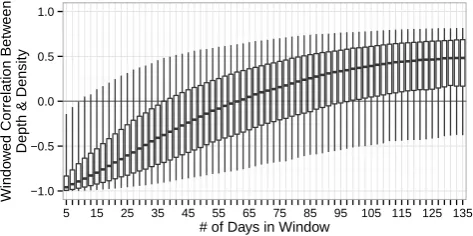
Figure 2 shows the correlation between density and depth as a function of timescale, for the period prior to peak SWE. The figure reveals that depth and density are strongly nega-tively correlated at timescales of 5–10 days (inner 50th quan-tile less than−0.8). In contrast, depth and density are weakly correlated at timescales longer than 60 days. For example, at 135 days, the median value of correlation is approximately 0.45 (with inner 50th quantile from roughly 0.2 to 0.6). Be-tween these two timescales, there is a shift from negative to positive correlation. The substantial range of correlation at all window sizes results from the different processes affect-ing depth and density and the variety of locations at which data are sampled. The shift from negative to positive correla-tion occurs at a timescale of approximately two months.
−1.0 −0.5 0.0 0.5 1.0
5 15 25 35 45 55 65 75 85 95 105 115 125 135
# of Days in Window
Windo
w
ed Correlation Betw
een
Depth & Density
Fig. 2. Correlation between snow depth and bulk density prior to
peak SWE as a function of window size (number of days used to compute the correlation). Ten thousand points were randomly se-lected from our full data set (described below) and odd-length win-dows around each expanded from 5 to 135 days for calculating the correlation whenever no more than 1 % of days were missing. Boxes represent the inner 50th quantile and whiskers the inner 90th quan-tile of correlations for each window. Because larger windows with less that 1 % missing points become more difficult to find prior to peak SWE for randomly selected points, the number of correlations over which boxplots are computed ranges from roughly 7000 at the 5-day window to 1500 at the 135-day window.
2.2 Existing models
A common approach to modeling snow bulk density is to be-gin with physical principles. The problem with this approach is that observed time series of many meteorological variables are required. For example, in the second snow model inter-comparison project (SNOWMIP2; Essery et al., 2009) only 2 models out of 33 did not require incoming shortwave ra-diation. Minimum requirements of even simple snow den-sity models, such as SNOW-17 of Anderson (1973) or that of De Michele et al. (2013), are time series of temperature and precipitation. A majority of snow depth measurements, including many automated measurements, do not have these accompanying observations, and including them can repre-sent significant expense.
The simplest approach to modeling snow bulk density is to derive a climatology. Mizukami and Perica (2008) justi-fied this approach by comparing the interannual variability of density and depth. They clustered climatological densi-ties from SNOTEL in the western US into 4 groups primar-ily distinguished by proximity to the Pacific Ocean, though with some geographical overlap between groups. They devel-oped a linear regression model of bulk density as a function of day, fitting coefficients in the 4 regions over two periods (December–February, March–April).
precipitation and air temperature were found to be most im-portant factors, though model parameters varied substantially by geographic region.
Jonas et al. (2009) and Sturm et al. (2010) developed snow bulk density models for the express purpose of converting observed depths to SWE. Both models use observed snow depth to predict a corresponding bulk density. The Sturm et al. (2010) model was intended as a general-purpose tool to convert observed snow depth to SWE in North America, pro-vided snow depth, day of year, and the snow class, as defined by Sturm et al. (1995). Sturm et al. (2010) calibrated their model separately for five broad snow classes (alpine, mar-itime, prairie, tundra, and taiga) and provided the parameters for application of their model across this domain.
The Jonas et al. (2009) model was developed using more than 5 decades of biweekly observations from the Swiss Alps. It was tuned monthly to both specific altitudes and ge-ographical regions in Switzerland. Though day of year (or month) is not a predictor in the Jonas model, time becomes an implicit predictor when selecting a training period. The intent of the model was not a general-purpose tool for pre-dicting snow density, but a demonstration of a methodology. Neither the Sturm et al. (2010) model nor the Jonas et al. (2009) model was designed for modeling snow density at the daily time step. Jonas et al. (2009) noted “that the model may not be suitable to convert time series of [depth] into SWE at daily resolution or higher. Transient phenom-ena such as the settling of recently fallen fresh snow cannot be comprehended by the model. Converted time series may therefore feature an incorrect fine structure in the temporal course of SWE.” Here, we develop a model explicitly de-signed to provide estimates of density on the daily timescale. As illustrated above, this will require accounting separately for the relationships between depth and density on short and long timescales.
In general, modeled density errors tend to be small. For ex-ample, both Jonas et al. (2009) and Sturm et al. (2010) high-light that modeled density errors yield SWE errors which ap-proximate those observed for repeat measurements due to lo-cal variability. The conservative nature of density means that, even when applied at the daily time step, the models provide reasonable estimates. Though only small statistical improve-ments are possible, we feel a model developed explicitly to represent daily variations in density is justified. To help in-form model selection by individual practitioners, we include discussion and evaluation of when the additional complexity of our new model is warranted.
3 Methodology
We evaluate the Jonas et al. (2009) and Sturm et al. (2010) density models (hereafter, the Jonas and Sturm models) with daily data to provide baselines for the development of an al-ternative model explicitly intended for use at a daily time
35 40 45
−120 −115 −110 −105
Longitude
Latitude
SNOTEL Stations
GPS Stations: # of SNOTEL within 70km
1−2
3−4
5−6
7−9
10−14
15−19
20−24
25−32
Fig. 3. Data used in this study come from the SNOTEL sites shown
in this figure. SNOTEL sites were selected if they were within 70 km of GPS snow depth stations. The number of SNOTEL sites within this radius of each GPS station is shown. Three GPS stations in Alaska, each with 1–2 associated SNOTEL sites, are not shown.
step (and because no such model currently exists.) Given our focus on the daily time step, our data sets and approach to training and evaluating the models differ from what was used in Jonas et al. (2009) and Sturm et al. (2010).
3.1 Data
The data set used to train and evaluate the models comes from SNOTEL stations (Serreze et al., 1999). Simultaneous observations of snow depth and SWE from selected SNO-TEL sites were manually quality controlled and (bulk) den-sity calculated as the ratio of SWE to depth. Only water years with at least 100 resulting density observations (be-tween days of year−92 and 181, or October–June, as in the Sturm model) were retained for model fitting. Gaps in daily time series were permitted.
Not all SNOTEL stations were used in our analysis. In-stead, we used only SNOTEL stations within 70 km of Plate Boundary Observatory GPS stations (Fig. 3) currently being used to estimate snow depth (Larson and Nievinski, 2013). The final data set contained 657 380 total observations of both depth and density at 345 SNOTEL sites in 19 differ-ent water years spanning 1994–2012. A total of 3370 water years were included.
with approximately daily temporal frequency (for exam-ple ground-based lidar surveys or ultrasonic depth measure-ments). A future study will report on applying the model to GPS sites and validation against in situ density observations. Several authors have noted systematic errors with SWE pressure measurements used by SNOTEL observations (Johnson and Marks, 2004; Meyer et al., 2012). We do not attempt to identify or correct any such errors, which would require temperature observations at the ground–snow inter-face or site-by-site comparison of SWE against accumulated precipitation. Also, because these studies indicated that mea-surement errors may be of both signs, it is prohibitively dif-ficult to reason about the impact of such errors on our re-sults. After the manual quality control mentioned above, we assume the SNOTEL measurements are accurate to within their observation resolutions. The resolution of the SNOTEL SWE measurements is 0.1 inches (0.254 cm), and that of snow depth is 1 inch (2.54 cm). Assuming these are our only sources of error, an error analysis of the calculated density over our full data set using half these accuracies as the error in each variable found 80 % of the density errors to be less than 1 % and 99.5 % of density errors to be less than 20 %.
Because our assumed errors (and perhaps systematic er-rors) are of smaller relative magnitude when SWE and depth are at a maximum, our validation will consider statistics re-stricted to a three-week window around peak SWE at each site and water year, in addition to statistics calculated for the full records at all sites. The peak-SWE period is important to many hydrologic applications.
3.2 Experimental design
For each SNOTEL site in the data set, we (1) retain only its location, snow depth, and date information; (2) identify the other SNOTEL sites in the data set which fall within 70 km of the current site; (3) train all three models (Sturm, Jonas, and ours) to all available depth and density observations at these other sites; (4) transfer the trained model parameters to the site of interest; (5) apply the model to estimate daily density from observed depths at the point of interest; and (6) generate (cross-validated) skill measures for both density and SWE estimation, bringing in the corresponding observations at the point of interest.
Our methodology evaluates the models under parameter transfer over scales of tens of kilometers. It is reasonable to believe that local training data (from within 70 km) are most appropriate for deriving and transferring model parameters to a point of interest (e.g., Mizukami and Perica, 2008; Sturm et al., 2010). However, a drawback of our general methodology is that it can only be used within 70 km of available training data. Our model is not for more general, geographical ap-plication, as in Sturm et al. (2010). Although it is possible with our model formulation, we did not stratify training data by elevation, as in Jonas et al. (2009), who found this step provided only modest improvements in model skill. When
fitting models, we combine all local data (i.e., within 70 km) equally, regardless of elevation.
Because we use local data to train the models, one might question if interpolation of concurrent density observations is easier than regression modeling and equally accurate. Re-gression modeling has the advantage of using historical data and does not require concurrent observations. Also, at the 70 km scale there may be important differences between snow depth time series at the locations where densities are observed and modeled. A regression model can account for such disparities in snow depth time series, which should lead to more robust estimates.
3.3 Jonas and Sturm models
Jonas et al. (2009) fit a simple linear regression model (Eq. 1), where density (ρ)is a linear function of depth (h)
and the parameters (a,b)are solved separately both monthly and over three elevation bands.
ρ (h,month, altitude)=a·h+b (1)
They also employed a further bias correction term in in-dividual regions. This step is not used in our study as we train the Jonas model for application to individual points in-stead of regions. As we also do not train on elevation bands, parameters are only a function of month (not altitude or re-gion). For each SNOTEL station location, we calibrate these 2 parameters for the 9 months (October–June).
Sturm et al. (2010) expressed density (ρ)as a function of depth (h)and day of year (DOY), and determined 4 general-purpose parameters (ρmax,ρ0,k1,k2) once and for all for
each of 5 snow classes (Sturm et al., 1995).
ρ (h,DOY, class)=
(ρmax−ρ0)·1−exp(−k1·h−k2·DOY)+ρ0 (2)
In our study, we calibrate the Sturm model once for each SNOTEL location using data from SNOTEL stations within 70 km, yielding 4 parameters for each point. Where Sturm et al. (2010) used a nonlinear, Bayesian analysis of covariance to fit their model, we employed constrained optimization. Our objective function was root mean square error (RMSE) of fit. Optimization was considered not to converge if the dif-ference between any parameter solutions at 1×10⁻⁷ preci-sion and 1×10⁻⁹precision was greater than 1 % of the range over all climate classes reported by Sturm et al. (2010).
3.4 A new model for daily applications
data were observed less frequently than biweekly and empha-sized the positive correlation of depth and density. Accord-ingly, both studies only reported positive coefficients. Based on the correlation of snow depth and density over different timescales and snow phases (Figs. 1 and 2), we expect these models to encounter difficulty when fitting their snow depth coefficients to daily data. During the ablation phase, a posi-tive correlation between depth and density is problematic in the Sturm model. Because the Jonas model is tuned monthly, it should perform better during the ablation phase. However, the depth coefficient in the Jonas model could be negative during the accumulation period when tuned to daily data over an interval of a month.
In developing a snow density model for daily applications, we chose to start from the Jonas model. Our first step is to derive a new set of predictor variables for the model. To ad-dress the problem of depth and density correlation on differ-ent timescales, we separate observed snow depth time series,
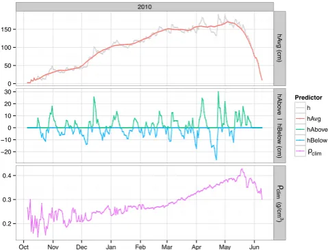
h, into two components or two new predictors of density. To model timescales of months, we use a moving window, of odd lengthW days, to average snow depths centered about the day to which the value is assigned. Days when depths are unavailable are omitted from the average, allowing for gaps in the time series. Because the first and last (W−1)/2 days of the time series have data only to one side and will often be positively biased, we do not average at these points but retain the observed depths. We call this new predictorhAvg. It is illustrated along with the observed time series,h, in the top panel of Fig. 4.
The next two predictors come from subtractinghAvg from the original depth time series (h) to get the differences, or anomalies, from the running average. Different physi-cal processes (accumulation versus compaction or melt) are dominant during periods with positive and negative anoma-lies. Therefore, we split these into two separate predictors,
hAbove and hBelow (Fig. 4). On days when the anoma-lies are negative, hAbove is set to zero. Likewise, when anomalies are positive hBelow is set equal to zero. These three new predictors transform the original snow depth time series,h, into long-range variability (hAvg) and into posi-tive (hAbove) and negative (hBelow) short-range anomalies. Their sum gives the original time series,h.
A second, more subtle problem with the Jonas and Sturm models used on a daily time step is a general deficiency in their overall shapes or structures. These will be discussed in the results section. While some of the issues stem from nega-tive correlation between depth and density in the ablation pe-riod, the Jonas model also exhibits discontinuities or jumps in density estimates between months when the model is trained. Though we do not include the methodology in our analysis, an unpublished modification to the original Jonas model has been implemented in practice which eliminates these discon-tinuities. (T. Jonas, personal communication and review of this paper, 2014). The modification requires estimating SWE
2010
0 50 100 150
−20 −10 0 10 20 30
0.2 0.3 0.4
hA
vg (cm)
hAb
ov
e | hBel
ow (cm)
(g/
cm
3
)
Oct Nov Dec Jan Feb Mar Apr May Jun
Predictor h hAvg hAbove hBelow clim
ρ
climρ
Fig. 4. Predictor variables for a new model of daily bulk density.
Example for Lake Irene SNOTEL site in 2010. The observed snow depth time series,h, is not used as a predictor but is transformed into three components. Long-range variability,hAvg, is shown in the top panel. Positive,hAbove, and negative, hBelow, anomalies of the observed time series,h, fromhAvg describe short-range variability. The sum of these three new predictors equalsh. The bottom panel shows the density climatology of fit,ρclim, which is derived from neighboring SNOTEL sites and used for both fit and prediction.
on the 15th day of each month and linearly interpolating it on to intervening snow depths before training the model.
To address structural problems, which may arise from fit-ting our daily model on a monthly basis, we investigate the incorporation of a daily density climatology of fit,ρclim, into
the model. The average density on each day over all data used to fit the model is applied as a predictor to both fit the model and in the subsequent prediction; this predictor comes strictly from the fitting data set. If any days are missing from the training set, these are linearly interpolated using their nearest neighbors. Figure 4 shows an example ofρclimfor the Lake
Irene SNOTEL site, based on the average from the 17 sta-tions within 70 km. Early- and flate-season fluctuasta-tions are due to greater natural variability during these periods or lack of data in some years. The general trend inρclimis to increase
until mid-May and then decline after that, after the snow is fully ripened. See Appendix A for more detailed discussion of density time series.
Having derived four new predictors of bulk density, our full daily model is expressed in Eq. (3):
ρ (h,month,neighbor)=
a·hAvg+b·hAbove+c·hBelow+d·ρclim+e.
temporal subset of them. However, the primary consideration for choosing bothW and the length of the training periods is the same, the availability of training data in each. If only one observation is available inW days to derive thehAvg predictor, then the anomaly terms (hAbove andhBelow) are zero. If there are no training observations in a training period, then parameters cannot be fit. For each training interval and choice ofW days for smoothing snow depth, five parameters are determined when fitting our regression model.
In this study, we choose to tune the model monthly to al-low for direct comparison with the published usage of the Jonas model. We also choose not to separate the model train-ing into accumulation and ablation periods of the snow-pack. This would likely only improve simulations after April, though it adds an extra layer of complexity. At the monthly timescale, most months are accumulation, the last is usually just ablation, and there may be a transitional month in some years. Finally, we limit the range of the regression mod-els (Jonas and ours) to the range of observed values. Esti-mates above or below these observed limits are set to the corresponding limit. This issue does not arise with the Sturm model.
We investigated eight models of intermediate complexity between the Jonas model and our full model. Our proposed model is more complex than the Jonas model, having five pa-rameters instead of two. There is potential to incrementally simplify our model towards the Jonas model by removing one or more predictors and their associated parameters. For example, one could simply use theρclimpredictor as an
ad-dition to the Jonas model or exclude it from our full model. These intermediate models would have three and four param-eters, respectively. Our evaluation of the intermediate mod-els (Appendix B) found the lowest RMSE under parameter transfer for our full model. Our full model was also partic-ularly insensitive to choice ofW and was minimized forW
greater than 17 days. Details are discussed in Appendix B. For the remainder of the paper we present results from our full model withhAvg computed during a 21-day window.
3.5 Model evaluation and comparison
Skill measures are calculated on the set of observations for which all models provide valid estimates. Our calibration of the Sturm model failed to converge at some stations, and ap-proximately 24 500 points were not estimated, or 3.7 % of the full data set. The Jonas model and our model failed at roughly 150 and 300 points, respectively. This occurs partic-ularly at the beginning and end of water years when there is not enough data to train the model for a given month or to calculate the running average or anomalies. Only 0.023 and 0.046 % of the full data set were not estimated by these mod-els. In the results below, statistics are computed on approx-imately 632 000 observations estimated by all three models. We also compute some statistics focusing on the three-week
2011 2012
0.1 0.2 0.3 0.4
0 10 20 30 40 50
Density (g/
cm
3
)
SWE (cm)
Nov Dec Jan Feb Mar Apr May JunNov Dec Jan Feb Mar Apr
Observations This paper Jonas et al. Sturm et al.
Fig. 5. Examples of observed and modeled density and SWE time
series in two water years at SNOTEL site 1145 Kilfoil Creek, UT. Depth and density values for depths less than 1.27 cm (0.5 in) are suppressed from the plot.
window centered on peak SWE in each water year. This sub-set includes 62 324 observations.
4 Results
4.1 Illustrative example
We begin with an illustrative example of important improve-ments offered by our model. These will be quantified in the following subsection. Figure 5 presents observed and mod-eled density and SWE time series at the Kilfoil Creek, UT, SNOTEL site for the 2011 and 2012 water years. This ex-ample demonstrates a range model of performance under different snow conditions. Snow accumulation in 2011 was roughly double that of 2012. In 2011, accumulation was on-going with large snowfall events in November and Decem-ber. In 2012, accumulation events were rare, with a single large event in January yielding a third of the maximum ob-served SWE. Both peak SWE and melt-out occurred a month earlier in 2012.
Viewed at the seasonal scale, all three models perform reasonably well in 2011. In 2012, the functional shape of the Sturm model is grossly inappropriate compared with the other two models. The Sturm model’s dependence on day of year results in overestimation of density by as much as 50 % at the beginning of March. The Jonas model and our model provide much better estimates for the entire 2012 season.
model fitting on a monthly basis results in unrealistic jumps in modeled density between months and systematic errors in both density and SWE.
Viewing the model estimates over timescales of days, den-sity variations associated with individual storms and melt events are missing from both the Sturm and Jonas mod-els. In contrast, our model captures much of the short-range variability in density. This results from covariances between snow depth and density at two separate timescales in our model. Not only is short-range covariance largely missing from the Sturm and Jonas models, but it is of the wrong sign (Fig. 5). This is most easily seen for the large accumulation event in the middle of January 2012 when SWE increased from approximately 10 to 17 cm. Both the Jonas and Sturm models have an associated increase in density with this accu-mulation, whereas our modeled density decreases in agree-ment with the observations. For the Jonas and Sturm models, large SWE errors are associated with this event because the density error is correlated with the change in snow depth. Though the modeled increases in density are small at short timescales in the example, the errors are large because ob-served density actually decreases. These errors are then mag-nified by the observed depth in the calculation of SWE. The same problems can be seen near peak SWE at the beginning of May 2012. Here the structural errors of the Jonas model, as applied at the daily time step, further exacerbate its density errors. Modeled peak SWE in 2012 is over 50 % greater than observed for the Sturm and Jonas models, while the estimate from our model is only 20 % too high.
The example in Fig. 5 also highlights the Sturm model’s systematic underestimation of density during the ablation phase. From mid-April to mid-May in 2011, the positive cor-relation of depth and density combined with the calibrated functional shape of the model result in density estimates that are too low. The extent of this problem will be revealed in the following subsection.
While our new model is by no means perfect, separation of the long- and short-range relationships between depth and density produces modeled variability, which closely tracks the observed densities and yields smaller density and SWE errors. The inclusion of the fitting climatology results in greater continuity of modeled density.
4.2 Model diagnostics
Table 1 presents three skill measures of modeled density and SWE for both the full data record and for the three weeks centered on peak SWE in each station and water year. Model density biases, important to verify because models are ap-plied under parameter transfer, are very small, less than a percent compared to observed densities. SWE biases are ef-fectively zero over the entire record. Near peak SWE, bias is nonzero but remains small, especially the Jonas model and our model.
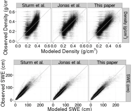
Fig. 6. Scatter plots of observed and modeled bulk density (top) and
SWE (bottom) for all 3 models.
Density RMSE is less than measurable and even smaller near peak SWE than over the full record. On the other hand, because density errors are multiplied by larger observed snow depths, SWE RMSE near peak SWE is greater than over the full record. RMSEs of both density and SWE im-prove, moving from the Sturm model, to the Jonas model, to our model. Relative to the Sturm model, the Jonas model and our model improve density RMSE by 5.6 and 9.9 %, respec-tively. Focusing on peak SWE, these improvements increase to 8 and 24 %. Relative to the Jonas model, our model yields a 4.5 % improvement in density RMSE over the full record and a 17.4 % improvement near peak SWE. Improvements in SWE RMSE are similar.
Coefficients of determination (R2)for both density and SWE also improve across models (Table 1). Near peak SWE, improvements in densityR2 are much greater. During this period, our model explains 16 and 13 % more of the ob-served density variability than the Sturm and Jonas mod-els, respectively. This corroborates that the model more ac-curately replicates daily variability in density, as illustrated in the previous section. The difference in theR2values be-tween density and SWE indicates the degree to which snow depth dominates estimation of observed SWE. Though 54– 44 % of the density variability over the full record remains unexplained by the models, only 6–4 % of the SWE variabil-ity is unaccounted for. At peak SWE, though more of the density variability is explained, SWER2 values are nearly identical to those over the full record because the magnitude of SWE is greater.
Table 1. Model skill statistics under parameter transfer for both the full record and a subset considering only the three weeks centered on
peak SWE for each station and water year.
Time period Statistic Variable Sturm et al. Jonas et al. This paper
Full record
Bias Density (g cm
−3) −0.001 0.000 0.000
SWE (cm) −0.21 −0.05 0.07
RMSE Density (g cm
−3) 0.071 0.067 0.064
SWE (cm) 7.1 6.7 6.3
R2 Density 0.46 0.52 0.56
SWE 0.94 0.95 0.96
Peak SWE
Bias Density (g cm−3) −0.015 0.000 −0.001
SWE (cm) −2.4 −0.2 0.3
RMSE Density (g cm−3) 0.050 0.046 0.038
SWE (cm) 8.4 7.8 6.5
R2 Density 0.55 0.58 0.71
SWE 0.95 0.95 0.96
Density (g/cm3) SWE (cm)
0 25 50 75
0.05 0.10 0.15 0 10 20 30
RMSE under parameter transfer at individual SNOTEL
Number of stations
Model This paper Jonas et al. Sturm et al.
Fig. 7. Distribution of RMSE in density and SWE at individual
SNOTEL stations.
sometimes constrained to the limits of the observed densi-ties. The correspondence between the observed and modeled densities is not great for any model, as described above by their coefficients of determination. In comparison, the scatter plots show the strong correspondence between modeled and observed SWE.
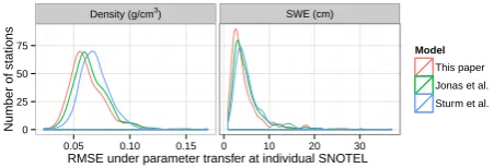
The statistics in Table 1 consider all modeled stations and water years simultaneously. Figure 7 shows the distribution of (full-record) RMSE over the individual SNOTEL stations. For both density and SWE, the RMSE distributions consis-tently shift to lower values, going from Sturm, to Jonas, to our model. The figure describes the probability of RMSE un-der parameter transfer as a function of model used. The tails of the distributions in Fig. 7 indicate that our model is some-times worse than the other models. Though worse than Sturm and Jonas in about 10 and 12 % of cases, our model’s rela-tive RMSE only exceeds 10 % in approximately 3 and 1 % of cases, respectively. Notably, the Sturm model performed much better in the few cases when less than 3 SNOTEL sta-tions, or less than approximately 3500 observasta-tions, were available to train the model.
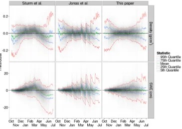
Density and SWE residuals (modeled–observed) are plot-ted as a function of day of year in Fig. 8. The figure reveals heteroskedasticity of the errors with day of year. The range
of density errors is greatest at the beginning and end of year, when snow depths are small and large fluctuations in density can occur in very short time periods. These are also times when observed density errors are the largest. The range of density errors is smallest in the month of February. The width of the inner 90th quantile of SWE errors increases with day of water year, while the width of inner 50th quantile is con-stant after April (though there are far fewer data points after May). Notably, the SWE errors do not follow the seasonal increase and decrease of snow depth.
Figure 8 reveals that the structural problems at the daily time step of the Sturm and Jonas models illustrated in Fig. 5 are common, rather than limited to that example. The Sturm model residuals become negatively biased at the beginning of April. By May the upper range of the 50th quantile nears zero, indicating a severe and systematic underestimation of density at the end of the year. This systematic underestima-tion during the melt period partially results from the posi-tive correlation of depth and density in the Sturm model. The sawtooth shape of the Jonas residuals indicates a sys-tematic progression from overestimation to underestimation across each month, starting in March and continuing through June. This results from tuning the models to daily data over each month. Subsequent, large jumps in the value of the residuals between months are also apparent. In contrast, our mean density residual deviates little from zero through the year. Deviations in the bias are typically found at the end of the months, similar to those of the Jonas model but of smaller magnitude. These persist because parameters in ad-jacent months are tuned independently. Though our model is not perfectly continuous in time, it is certainly an improve-ment over the continuity of the Jonas model. These disconti-nuities are clearer in our SWE residuals beginning in May.
Fig. 8. All model residuals (modeled–observed) in density (upper panel) and SWE (lower panel) as a function of day of water year for each
model. Green line shows mean error, blue lines indicate the inner 50th quantile of error, and the red lines the inner 90th quantile of error.
Table 2. Nonexceedance probabilities for a range (of absolute
value) of percent error calculated for three-week windows centered on peak SWE. Numbers apply to both density and SWE as depth is observed and assumed to be correct. Jonas et al. (2009) cite typical values of density measurement error as 15–20 %.
Empirical probability of nonexceedance during 3 weeks centered on peak SWE
Absolute value Sturm Jonas This paper
of percent error
5 0.25 0.27 0.30
10 0.48 0.50 0.56
15 0.66 0.68 0.75
20 0.80 0.80 0.86
25 0.88 0.88 0.93
30 0.93 0.92 0.96
each year. Both Jonas et al. (2009) and Sturm et al. (2010) evaluated their models in terms of percent error. They com-pared these errors to errors associated with repeated obser-vations at a single location. Table 2 shows the likelihood of modeled absolute percent error not exceeding thresholds be-tween 5 and 30 %. (Note that, because depth is observed, percent error is the same for density and SWE.) At the time of peak SWE, we again see consistently better performance
moving from the Sturm model to the Jonas model, and to our model. Our model resulted in no more than 15 % error 75 % of the time, whereas the Jonas and Sturm models did not exceed this threshold 68 and 66 % of the time, respec-tively. Both the Sturm and Jonas models keep 80 % of esti-mates to less than 20 % error, while our model manages to do this 86 % of the time. That is, for dates near peak SWE, our model has almost one-third less errors beyond the typically observed range of 20 % error.
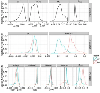
4.3 Model parameters
conditions and long-timescale negative correlation between depth and density.
The coefficients of depth (h)in the Jonas and Sturm mod-els are distributed similarly as the coefficients ofhAvg in our model. In contrast, the Sturm coefficients cover a slightly wider range of values. In the Jonas model, the values of the intercept term increase with month and govern minimum modeled densities. In our model, the intercepts interact with the coefficient ofρclim. In April, coefficients ofρclimare
dis-tributed around one and the intercepts around zero. In Jan-uary, intercepts are positive and distributed about 0.1, while the coefficients ofρclimare distributed about 0.5.
5 Discussion
The skill measures presented above indicate that our model yields improvements over the existing models when evalu-ated at the daily time step. The Jonas and Sturm models were not intended for daily applications. The example shown in Fig. 4 highlights their shortcomings at this timescale, which are largely resolved using our formulation.
5.1 Contextualizing skill improvements
Even though our model offers more realistic density estima-tion at the daily time step, the skill improvements are not large (e.g., in terms of RMSE). There are two reasons why it is difficult to significantly improve the model skill. First, density is a conservative variable: it is naturally constrained between fairly narrow limits and only approaches these lim-its in certain circumstances. This is the premise of such a simple approach to modeling density from depth. Because model errors are rarely large, there is little room for improve-ment. Second, we have evaluated the models under parame-ter transfer: data from the station where density is estimated and evaluated are not used to fit the model. This provides an added challenge to estimation but provides a more realistic evaluation in terms of applications, for example converting GPS-derived snow depth into SWE at locations where den-sity observations are not available. Parameter transfer is a challenge of the application rather than a shortcoming of the models.
For additional insight on the models’ ability to accurately represent the relationship between depth and density, we evaluate each without (spatial) parameter transfer. Instead of fitting the model at nearby sites and transferring the param-eters to the site of interest, we now fit the models to density observations at the site of interest and evaluate modeled den-sity and SWE over all years at this location. Because denden-sity climatology (ρclim) is a predictor in our model, we fit the
model separately for each year while dropping the year to be estimated from the training data set (leave-one-out validation on a water year basis). We do not apply this cross-validation to the Sturm and Jonas models because it will have
a negligible effect. This procedure is more stringent for our model, but only slightly penalizes years with extreme densi-ties. Unlike for parameter transfer, model assessment at the location of fit is not confounded by differences between sites (up to 70 km apart) due to elevation, slope/aspect, vegetation, etc.
Table 3 shows skill statistics of fit for the three models and skill improvements compared to skill statistics under pa-rameter transfer. As expected, fitting the regression (Jonas and our) models completely eliminates bias (not shown). The Sturm model retains a very small bias because optimiza-tion did not minimize bias, only RMSE. The model statis-tics in Table 3 improve moving from the Sturm model to the Jonas model to our model, but these improvements are considerably greater than under parameter transfer. Now our model explains 19 % more variance in density, for a total of (R2=)75 % variance explained. The Jonas and Sturm mod-els have R2increases of 14 and 12 %, respectively, yielding 66 and 58 % variance explained. The strong improvement for our model indicates that it more appropriately captures the relationship between density and depth when applied at the daily timescale. These improvements also illustrate the skill penalty associated with parameter transfer.
5.2 Why not use our model?
In this study, we have only investigated parameter transfer over scales of tens of kilometers. We do not consider mod-eling density at distances further than 70 km from the near-est SNOTEL site (or site with similar data). Therefore, our results do not apply to locations on the scale of hundreds of kilometers from locations with density data required for model training. In the Results section we also noted better average performance of the Sturm model as used in this study when less than three nearby (within 70 km) stations were available to train the model. This result suggests that using the Sturm model is preferred when training data are either limited locally or when only available far from the site at which density will be estimated. At the same time, we illus-trated a general problem with the relationship between den-sity and depth in the Sturm model during the melt phase. Improvements to the general approach of Sturm et al. (2010) might be gained if the model were tuned separately for accu-mulation and ablation phases.
(h) (DOY)
0.00 0.25 0.50 0.75 1.00
Stu
rm et al.
−0.004
−0.0020.000 0.0020.0030.0040.0050.006 0.21 0.24 0.27 0.3 .57 0.60 0.63 0.66
Scaled
Ke
rnel Density
(h) intercept
0.00 0.25 0.50 0.75 1.00
Jonas et al.
−0.003 −0.002 −0.001 0.000 0.001 0.002 0.2 0.3 0.4 0.5
Scaled
Ke
rnel Density
(hAvg) (hAbove) (hBelow) intercept ( )
0.00 0.25 0.50 0.75 1.00
This paper
−0.002
−0.0010.0000.0010.002 −0.010−0.0050.000 −0.0050.0000.005 −0.2 0.0 0.2 0.0 0.5 1.0 1.5
Scaled
Ke
rnel Density
Month Jan Apr
clim ρ 0
ρ ρmax
Fig. 9. The distribution of model parameters over all SNOTEL sites. If the parameter is the coefficient of a predictor, the predictor name
is shown in parentheses. Otherwise the parameter name is given. Top panel is the Sturm model, middle panel is the Jonas model, and the bottom panel is the model developed in this paper.
Table 3. Model statistics of fit (not under parameter transfer). Improvements compared to parameter transfer statistics are indicated by1.
Statistic Variable Sturm et al. (2010) Jonas et al. (2009) This paper
RMSE Density (g cm
−3) 0.062 (1= −0.009) 0.055 (1= −0.012) 0.048 (1= −0.016)
SWE (cm) 5.57 (1= −1.50) 4.66 (1= −2.05) 3.79 (1= −2.56)
R2 Density 0.58 (1=0.12) 0.66 (1=0.14) 0.75 (1=0.19)
SWE 0.96 (1=0.02) 0.97 (1=0.02) 0.98 (1=0.02)
the same degraded data sets, our model has consistently 4 % lower RMSE under parameter transfer when data are avail-able every two or three days. The two models perform sim-ilarly when data are available every five days. For weekly data, our model had 8 % worse RMSE compared to the Jonas model. The snow depth time series used in this study con-tained gaps, so the data frequency was not always daily and the degraded time series potentially less frequent than in-tended. These gaps in the snow depth inputs also imply that the statistics reported for our model might improve if data were available every day.
5.3 Further improvements and research problems
Several potential improvements to our model were not ex-plored here. We tune the model monthly and do not explicitly separate coefficients ofhAvg for snow ablation and accumu-lation phases, though they are likely different. Alternatively, we could tune the model more frequently in time. Further, because the magnitude of change in bulk density depends on the relative amounts of existing snowpack and accumulation or ablation, a more detailed model might consider ratios of anomalies to smoothed depth, though it will require manag-ing division by zero. A more inventive, different approach to smoothing could also help distinguish true positive and neg-ative anomalies.
We have not considered real-time applications. We pre-sented results using a 21-day moving window to calculate smoothed snow depth and anomalies centered on a given date. In real time, this window reaches into the future. We do not know how well a retrospective window for a given date would work. It is something worth investigating, though most applications of SWE (or density) can likely wait 10 days for an improved estimate.
Widespread application of our daily density model is hin-dered by the use of local (∼70 km) data for fitting model pa-rameters and deriving the climatology of fit. We have charac-terized model accuracy/errors only for this scenario. A study of model sensitivity to proximity of training data, the ef-fects of physiographics on model parameters, and to predic-tor variable quality would provide greater context for wider applications. While measurements of the spatial variability of snow depth have improved drastically with the advent of lidar measurement techniques (McCreight et al., 2014), the spatial variability of bulk density remains poorly understood (López-Moreno et al., 2013). In this study, we have consid-ered the spatial variability of density over scales of tens of kilometers. However, the density observations in this study come from SNOTEL sites, which have their own kind of ho-mogeneity when compared to the larger environment. They are most commonly located in forested, subalpine locations. Our findings are likely to be more representative of these lo-cations as opposed to unforested or wind-exposed lolo-cations (e.g., Clow et al., 2012). Transferring parameters derived at SNOTEL sites to snow depth measurement locations such as for GPS, which are necessarily unforested and tend to be at lower elevations, may introduce model bias. Though some issues related to parameter transfer can be studied with SNOTEL observations, understanding parameter transfer in a broader context may require new and physiographically di-verse time series observations of snow bulk density.
Alternatively, our model might also be explored or ex-tended using hybrid approaches. Model sensitivity to more general climatologies similar to those estimated by Borman et al. (2013) could be investigated. Physical models could also provide simulated data or climatologies over a wide va-riety of physiographic conditions. Our statistical model could
be fit to synthetic data to explore its sensitivity or to develop general-use parameters (e.g., Sturm et al., 2010).
While a strength of our model is the requirement of only snow depth observations, the associated drawback is that energy-related processes are not explicitly included via pre-dictor variables. Energy-related processes explain a large fraction of bulk density variability at long timescales (e.g., Chen et al., 2010) and are only implied via their relationship with snow depth variability and the climatology of fit. Be-cause air temperature can be easily measured or estimated with reasonable accuracy, it seems that the best way to im-prove our model formulation with additional observations would involve adding an air (or other) temperature variable. Research would be required to understand how such obser-vations would most appropriately modify the current terms. Successful inclusion of an air temperature predictor in the model would likely improve transferability of parameters be-tween physiographically dissimilar locations. Temperature observations might also be used to constrain changes in den-sity or SWE to physically realistic scenarios.
6 Conclusions
We developed a model for converting snow depth observa-tions to bulk density estimates at the daily timescale. Our model improves the estimation of bulk density and SWE from daily snow depth, compared to existing approaches that were not intended for daily application. Our main innova-tion was separating the short- and long-timescale covariances between snow depth and density, which are negatively cor-related at short (10 days) timescales while positively corre-lated at longer (90 days) timescales. Snow depth variability at long timescales was modeled using a running mean and variability at short timescales by observed anomalies from the mean. A climatology of fit was also included as a pre-dictor variable. The model exhibited improved statistics and qualitatively more-realistic behavior under parameter trans-fer when fitting models to data within a 70 km radius of the modeled location. The model showed even greater improve-ments when fit at the modeled location (parameters not trans-ferred), explaining 75 % of the observed density variability in 632 000 observations. We recommend using the model under parameter transfer whenever it can be trained to at least three sites and applied to observations more frequent than one in five days.
Acknowledgements. This research was supported by
NSF-EAR 1144221, NSF-NSF-EAR 0948957, and NASA NNX12AK21G. Thanks to Kristine Larson for impetus and for support for our research. Two anonymous referees and T. Jonas provided insight-ful reviews, which greatly improved this paper. H. P. Marshall also contributed valuable comments and discussion.
packages (Wickham, 2007, 2009, 2011), were used for analysis and presentation.
Edited by: E. Larour
References
Anderson, E. A.: National Weather Service river forecast system– snow accumulation and ablation model, Technical memorandum nws hydro-17, November, 1973, 217 pp., 1973.
Beniston, M.: Climatic change in mountain regions: a review of pos-sible impacts, in: Climate Variability and Change in High Ele-vation Regions: Past, Present & Future, 5–31, Springer Nether-lands, 2003.
Bormann, K. J., Westra, S., Evans, J. P., and McCabe, M. F.: Spa-tial and temporal variability in seasonal snow density, J. Hydrol., 484, 63–73, doi:10.1016/j.jhydrol.2013.01.032, 2013.
Chen, X., Wei, W., and Liu, M.: Change in fresh snow density in Tianshan Mountains, China, Chinese Geogr. Sci., 21, 36–4, 2011.
Clow, D. W., Nanus, L., Verdin, K. L., and Schmidt, J.: Evaluation of SNODAS snow depth and snow water equivalent estimates for the Colorado Rocky Mountains, USA, Hydrol. Processes, 26, 2583–2591, 2012.
Cohen, J. and Entekhabi, D.: The influence of snow cover on North-ern Hemisphere climate variability, Atmos.-Ocean, 39, 35–53, 2001.
Deems, J. S. and Painter, T. H.: Lidar measurement of snow depth: accuracy and error sources, in: Proceedings of the 2006 Interna-tional Snow Science Workshop: Telluride, Colorado, USA, Inter-national Snow Science Workshop, 330–338, 2006.
De Michele, C., Avanzi, F., Ghezzi, A., and Jommi, C.: Investigat-ing the dynamics of bulk snow density in dry and wet conditions using a one-dimensional model, The Cryosphere, 7, 433–444, doi:10.5194/tc-7-433-2013, 2013.
Doesken, N. J. and Judson, A.: The Snow Booklet: A guide to the science, climatology, and measurement of snow in the United States, Colorado Climate Center, Department of Atmospheric Science, Colorado State University, 1997.
Essery, R., Rutter, N., Pomeroy, N., Baxter, R., Stahli, M., Gustafs-son, D., Barr, A., Bartlett, P., and Elder, K.: SNOWMIP2: An evaluation of forest snow process simulations, Am. Meteorol. Soc, 90, 2009. 1120-1135.
Garvelmann, J., Pohl, S., and Weiler, M.: From observation to the quantification of snow processes with a time-lapse camera network, Hydrol. Earth Syst. Sci., 17, 1415–1429, doi:10.5194/hess-17-1415-2013, 2013.
Gutmann, E. D., Larson, K. M., Williams, M. W., Nievinski, F. G., and Zavorotny, V.: Snow measurement by GPS interferometric reflectometry: an evaluation at Niwot Ridge, Colorado, Hydrol. Process., 26, 2951–2961, 2012.
Harpold, A. A., Guo, Q., Molotch, N., Brooks, P., Bales, R., Fernandez-Diaz, J. C., Musselman, K. N., Swetnam, T., Kirch-ner, P., Meadows, M., Flannagan, J., and Lucas, R.: A LiDAR de-rived snowpack dataset from mixed conifer forests in the Western US, Water Resour. Res., doi:10.1002/2013WR013935, in press, 2014.
Johnson, J. B. and Marks, D.: The detection and correction of snow water equivalent pressure sensor errors, Hydrol. Process., 18, 3513–3525, 2004.
Jonas, T., Marty, C., and Magnusson, J.: Estimating the snow water equivalent from snow depth measurements in the Swiss Alps, J. Hydrol., 378, 161–167, 2009.
Larson, K. M. and Nievinski, F. G.: GPS snow sensing: results from the EarthScope Plate Boundary Observatory, GPS solutions, 17, 41–52, 2013.
Larson, K. M., Gutmann, E. D., Zavorotny, V. U., Braun, J. J., Williams, M. W., and Nievinski, F. G.: Can we measure snow depth with GPS receivers?, Geophys. Res. Lett., 36, L17502, doi:10.1029/2009GL039430, 2009.
López-Moreno, J. I., Fassnacht, S. R., Heath, J. T., Musselman, K. N., Revuelto, J., Latron, J., Morán-Tejeda, E., and Jonas, T.: Small scale spatial variability of snow density and depth over complex alpine terrain: Implications for estimating snow water equivalent, Adv. Water Resour., 55, 40–52, 2013.
McCreight, J. L., Slater, A. G., Marshall, H. P., and Rajagopalan, B.: Inference and uncertainty of snow depth spatial distribution at the kilometre scale in the Colorado Rocky Mountains: the effects of sample size, random sampling, predictor quality, and validation procedures, Hydrol. Process., 28, 933–957, 2014.
Meyer, J. D. D., Jin, J., and Wang, S. Y.: Systematic Patterns of the Inconsistency between Snow Water Equivalent and Accumulated Precipitation as Reported by the Snowpack Telemetry Network, J. Hydrometeorol., 13, 1970–1976, 2012.
Mizukami, N. and Perica, S.: Spatiotemporal characteristics of snowpack density in the mountainous regions of the western United States, J. Hydrometeorol., 9, 1416–1426, 2008.
Parajka, J., Haas, P., Kirnbauer, R., Jansa, J., and Blöschl, G.: Poten-tial of time-lapse photography of snow for hydrological purposes at the small catchment scale, Hydrol. Process., 26, 3327–3337, 2012.
Prokop, A., Schirmer, M., Rub, M., Lehning, M., and Stocker, M.: A comparison of measurement methods: terrestrial laser scanning, tachymetry and snow probing for the determination of the spatial snow-depth distribution on slopes, Ann. Glaciol., 49, 210–216, 2008.
R Development Core Team R: A language and environment for sta-tistical computing, Vienna, Austria: R Foundation for Stasta-tistical Computing, 1–1731, 2008.
Ryan, W. A., Doesken, N. J., and Fassnacht, S. R.: Evaluation of ultrasonic snow depth sensors for US snow measurements, J. At-mos. Ocean. Technol., 25, 667–684, 2008.
Serreze, M. C., Clark, M. P., Armstrong, R. L., McGinnis, D. A., and Pulwarty, R. S.: Characteristics of the western United States snowpack from snowpack telemetry, SNOTEL data, Water Re-sour. Res., 35, 2145–2160, 1999.
Sturm, M., Holmgren, J., and Liston, G. E.: A seasonal snow cover classification system for local to global applications, J. Climate, 8, 1261–1283, 1995.
Sturm, M., Taras, B., Liston, G. E., Derksen, C., Jonas, T., and Lea, J.: Estimating snow water equivalent using snow depth data and climate classes, J. Hydrometeorol., 11, 1380–1394, 2010. Wickham, H.: Reshaping Data with the reshape Package, J. Statist.
Softw., 21, 1–20, 2007.
Wickham, H.: ggplot2: elegant graphics for data analysis, Springer Publishing Company, Incorporated, 2009.
Appendix A
More detailed empirical relationships between depth and density
In Fig. 1, we simplified our discussion of depth and den-sity by focusing on the period from Feb to May. To more completely characterize the relationship between density and depth, we reveal the full water years from Fig. 1 in Fig. A1 and divide the snow season into four phases. These are distin-guished by three vertical, dashed lines in each water year. In chronological order, we call these phases the early accumu-lation phase, the main accumuaccumu-lation phase, the main abaccumu-lation phase, and the late ablation phase. Figure 1 concentrated on the main accumulation and ablation phases, which are distin-guished by peak SWE or snow depth. The early accumulation phase is characterized by markedly higher variability in den-sity because the total SWE or depth is still low. Though it can vary between sites and years, snow depth accumulations over 50 cm typically mark the end of the early accumulation phase. The main ablation phase is distinguished from the late ablation phase by a switch from increasing to constant (or perhaps decreasing) density. This switch occurs with the ripening of the snowpack, when it holds a maximum amount of liquid water. In the example time series (Fig. A1), the early accumulation constitutes roughly 20 % of the 9-month water year while the late ablation phases is roughly 5 % of the water year. The main accumulation and ablation phases represent approximately 60 and 15 % of the water year, respectively. It is important to note that we present an example analysis for a single location in two different years. Different locations and even different years could have drastically different distribu-tions of these snow phases. Sites with ephemeral snowpack may not have main accumulation or main ablation phases.
2010 2011
0 100 200 300 400 500
Oct Nov Dec Jan Feb Mar Apr May Jun Jul Oct Nov Dec Jan Feb Mar Apr May Jun Jul
Sn
ow Depth (cm)
|
Bulk Density (kg/
m
3 )
Bulk Density Snow Depth
Fig. A1. Data from the Lake Irene SNOTEL site in northern Colorado. Both water years are separated into 4 phases by vertical dashed lines:
early accumulation, main accumulation, main ablation, and late ablation.
Appendix B
Model selection
In the methodology section, we developed new predictors for use in regression modeling and we justified our choice of the full model as presented in Eq. (3). However, between the Jonas et al. (2009) and our full model, a range of intermedi-ate models exist, using various combinations of the available predictors from the two models. In this appendix we examine the performance of these intermediate models.
The full set of predictors we consider are intercept,snow depth (h), smoothed snow depth (hAvg), observed anoma-lies from smoothed snow depth (hAvgDiff), positive and neg-ative anomalies from smoothed snow depth (hAbove and
hBelow), and density climatology of fit (ρclim). The time
se-ries of anomalies, hAvgDiff, is calculated as h−hAvg. It is not split into positive and negative anomalies, as is the case forhAbove and hBelow. The hAvgDiff term was not included in Eq. (3), or in the analyses in the main part of the paper. Figure B1 compares the Jonas and Sturm models with models of intermediate complexity. Models are evaluated us-ing RMSE under parameter transfer over the entire data set. The figure shows RMSE as a function ofW, the number of days used to compute average snow depth and its associated anomalies. The Sturm and Jonas models are independent of
W, as is the Jonas model with the addition of the density cli-matology of fit,ρclim. The Jonas model has a smaller set of
residuals (RMSE) than the Sturm model, and the addition of the climatology of fit predictor improves the Jonas model.
0.064 0.066 0.068 0.070
3 10 20 30 35
Window size (days)
RMSE in density under pa
ram t
rans
fer (g/
cm
3 )
Model Sturm Jonas Jonas: hAvg:hAvgDiff hAvg:hAbove hAvg:hBelow hAvg:hAvgDiff: hAvg:hAbove: hAvg:hBelow: hAvg:hAbove:hBelow hAvg:hAbove:hBelow:
clim
ρ
clim
ρ
clim
ρ
clim
ρ
clim
ρ
Fig. B1. Comparison of model RMSE in density (over all observations) under parameter transfer as a function of window size for computing
the running mean of snow depth predictorhAvg and the associated predictorshAvgDiff (all anomalies),hAbove (positive anomalies), and hBelow (negative anomalies).ρclimis the daily density climatology of fitting data predictor.
The remaining models (grey and red) involve windowed average snow depth (hAvg) and depend on the window size. The figure reveals that the full model, shown in red, improves upon all intermediate models (shown in grey and differenti-ated with symbols) for window sizes greater than 17 days. The full model dropping thehBelow term is competitive for shorter averaging windows, but the RMSE of the full model is lower for averaging windows greater than 17 days. The full model shows improvement over the models which do not in-volve averaging snow depth: Sturm, Jonas, and Jonas:ρclim.