Convolutional Neural Networks Applied on Weather Radar Echo Extrapolation

2017 International Conference on Computer Science and Application Engineering (CSAE 2017) ISBN: 978-1-60595-505-6

Convolutional Neural Networks Applied on

Weather Radar Echo Extrapolation

En Shi, Qian Li*, Daquan Gu and Zhangming Zhao

College of Meteorology and Oceanography, National University of Defense Technology, China

ABSTRACT

Extrapolation technique of weather radar echo possesses a widely application prospects in short-term nowcast. The traditional methods of radar echo extrapolation are difficult to obtain long limitation period and lacking in utilization rate of radar data. To solve this problem, this paper proposes a method of weather radar echo extrapolation based on convolutional neural networks (CNNs). In order to adapt the strong correlation between weather radar echo images of contiguous time, on the basis of traditional convolutional neural networks, this method present a new CNNs model, namely, Recurrent Dynamic Convolutional Neural Networks (RDCNN). RDCNN consists of recurrent dynamic sub-network and probability prediction layer, and constructs a cyclic structure in the convolution layer, which improve the ability of RDCNN to process time-related images. In the experiments of radar data from Nanjing, Hangzhuo and Xiamen, compared with traditional methods, this method has achieved higher accurate of extrapolation and extended the limitation period effectively, which meets the requirement for application.

INTRODUCTION

Nowcasting convective precipitation has long been an important problem in the field of weather forecasting, especially for preventing disaster weather [1]. The goal of precipitation nowcast is to make prediction of rainfall intensity precisely and timely in local region over relatively short period of time. Since precipitation nowcast requires for more accurate forecasting resolution and time than other traditional rainfall or temperature predictions, this challenging operation has emerged as a popular research topic in the meteorologic field [2]. At present, the extrapolation forecast based on radar echoes is the mainstay of precipitation nowcast [3,4], more accurate and efficient predicted radar echos are crucial for improving the accuracy of short-term precipitation nowcast. The purpose of the radar echo extrapolation is to predict the future position and intensity of the radar echo based on the current radar observations[5]. The key to radar echo extrapolation is to obtain a reliable extrapolated echo image. The essence of radar echo extrapolation is based on the current and historical moments of radar echo images to predict next, unseen one. Existing methods for radar echoes extrapolation can roughly be categorized into two classes, centroid tracking methods and TREC (Tracking Radar Echoes by Correlation) methods [5,6,7].

calculating the correlation of radar echoes at previous several moments. Based on the TREC methods, the researchers further developed COTREC (Continuity of TREC vectors) and DITREC (Difference Image based TREC) along with other methods, which widely used in precipitation forecasting. However, this TREC methods only based on past several radar echo images to predict the next radar echo image, which is defective in data utilization. And the effective forecast time usually can not exceed one hour.

To solve this problem, we examine this challenging weather forecasting operation from machine learning and propose a method of weather radar echo extrapolation based on convolutional neural networks (CNNs).In recent years, there have been few studies on CNNs applied to weather forecasting. Xingjian et al. [8] proposed the convolutional LSTM (ConvLSTM) by adding the convolutional structures in fully connected LSTM (FC-LSTM). Singh et al. [9] uses convolutions within recurrence structure in recurrent neural networks exploiting both spatial and temporal dependencies in the data, which achieved state-of-the-art performance while reducing the model size by 4 times compared with the conventional model. This paper presents a new CNNs model, namely, recurrent dynamic convolutional neural networks (RDCNN). Specifically, observing that a radar image in the sequence can be usually approximated as a translation of the previous image in the sequence, CNNs in this paper is trained by a variety of weather radar images sorted by time to learn about how echoes translate and predict the next radar image in the sequence. To accommodate the strong correlation between radar echo images at adjacent times, we modify the network structure on the basis of traditional CNNs, so that the convolution kernels can save the history training information in the training process, and the convolution kernels vary from input to input during testing. RDCNN is more suitable for the radar echo extrapolation in process a series of time-related image sequences.In the comparison experiment, we compare the prediction of RDCNN to other baselines, including the ripe COTREC method. We show that by using RDCNN, we gain the improvement in accuracy of predictions compared to the other baselines.

PRELIMINARIES

Convolutional Neural Networks (CNNs)

In recent years, convolutional neural networks are becoming increasingly popular in solving various computer vision applications, such as: object recognition, objection localization, cancer detection and face recognition [10,11,12,13]. What sets CNNs apart from other neural networks are the use of the convolutional layer and the sampling layer [10]. The convolutional layer computes the output feature maps by convolving the feature maps of the previous layer with a set of convolution kernels, and the sampling layer reduces the resolution of its input feature maps [14,15]. The convolutional layer computes the output feature via the following equations:

* +

j ij i j

i M

y f k x b



 

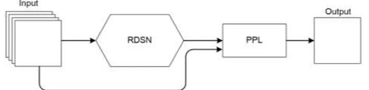
Figure 1. The architecture of RDCNN. RDSN is a sub-network which computes the probability vectors. The last image in the sequence and the probability vectors then input into PPL to predict the next radar

echo image.

where ( )f is an element-wise non-linearity, such as a sigmoid or hyperbolic tangent, M is the set of input feature maps, x_i is the i-th input feature map, y_j is the j-th output

feature map, bj is the j-th bias, the convolution kernels would be denoted by kij and

the * symbol is the convolution operator. The sampling layer computes the output feature via the following equations:

( )

j i

y



g x

where ( )g is a sampling function, such as Mean-pooling or Max-pooling.

Recurrent Neural Networks (RNNs)

The conventional neural networks are difficult to deal with time-related data. Recurrent neural networks (RNNs) are a class of artificial neural network where connections between units form a directed cycle [16]. This allows it to exhibit dynamic temporal behavior. Unlike feedforward neural networks, RNNs can use their internal memory to process arbitrary sequences of inputs. This makes them applicable to tasks such as speech recognition [17] or text recognition [18].

RNNs store historical training information through the cyclic structure. Radar echo extrapolation is to process time-dependent image sequences. By referring to the cyclic structure of RNNs, it is possible to enhance the ability of the network to process timing-related image sequences.

RECURRENT DYNAMIC CONVOLUTIONAL NEURAL NETWORK (RDCNN) MODEL

Figure 2. The cyclic structure in RDSN consists of convolution layers and hidden layers.

Recurrent Dynamic Sub-network(RDSN)

Recurrent dynamic sub-network is the main part of RDCNN, which is a separate CNNs model. The radar image sequence is input into the RDSN, and two one-dimensional vectors are calculated by the convolution layers, the sampling layers and the classifier. In RDSN, the hidden layer and the convolution layer make up the cyclic structure. The cyclic structure in RDSN is shown in Figure 2. In the cyclic structure, the convolution layer is connected with the hidden layer, the output feature maps of the convolution layer is processed by the hidden layer, after that, the information is re-entered into the convolution layer at the next time step.

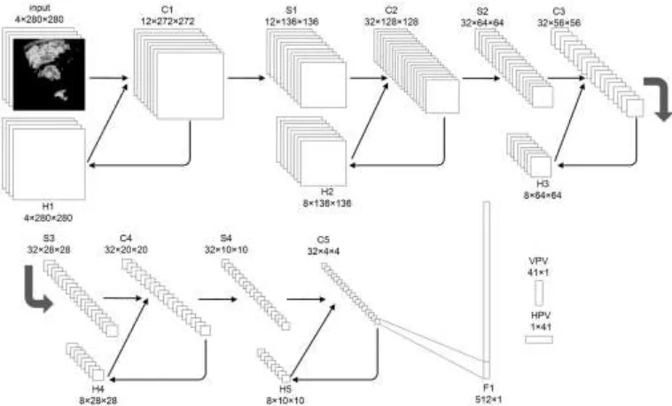
The overall structure of RDSN is shown in Figure 3. The four radar images of size 280×280 are given as inputs to a convolutional layer (C1) with 12 convolution kernels of size 9×9. The resulting 12 feature maps are then passed to a sampling layer (S1) and a hidden layer (H1), S1 takes the max over 2×2 spatial blocks with a stride of 2, and H1 with 4 convolution kernels of size 9×9 compute 4 feature maps that input into C1 at next time step. The next 3 convolutional layers (C2, C3, C4) contain 32 filters of size 9×9. The resulting 32 feature maps are then passed to its next sampling layer and hidden layer, the sampling layers (S2, S2, S4) take the max over 2×2 spatial blocks with a stride of 2, and the hidden layers (H2, H3, H4) with 8 convolution kernels of size 9×9 compute 8 feature maps that input into corresponding convolutional layers at next time step. This is followed by another conventional convolutional layer (C5) with 32 filters of size 7×7. The resulting 32 feature maps are then passed to a classifier (F1) and a hidden layer (H5), H5 with 8 parameters compute 8 feature maps that input into C5 at next time step, and F1expands the feature maps into a column vector of size 521 × 1, then apply softmax function to the column vector to calculate two probability vectors, VPV and HPV. Due to the characteristics of the softmax function, VPV and HPV are positive and sum to 1, which could be considered as vectors of probabilities.It should be noted that when calculating the output feature maps the hidden layer, we need zero padding to ensure that the resolution of output maps match with the input maps of convolution layer.

Probability Prediction Layer (PPL)

Figure 3. The overall structure of RDSN with five convolutional layers (C1, C2, C3, C4, C5), four sampling layers (S1, S2, S3, S4), five hidden layers (H1, H2, H3, H4, H5) and one classifier.

Figure 4. The structure of PPL. DC1 takes the last image in the sequence and convolves it with VPV, DC2 takes the output of DC1 and convolves it with HPV to compute the next radar echo image.

final predicted image. Figure 4 shows how PPL works. It contains two network layers of DC1 and DC2. The vertical probability vector VPV is taken as the convolution kernel of DC1 and convoluted with the last image in the sequence to get the feature map of size 240 280 . The horizontal probability vector HPV is the convolution kernel of DC2 and convoluted with the obtained feature map from DC1 to predict the next radar echo image.

EXPERIMENTS

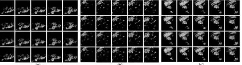
Figure 5. Three prediction examples. All the predictions and ground truths are sampled with an interval of 6 min. From top to bottom: input frames; ground truth frames; prediction by RDCNN; prediction by COTREC. (a) Nanjing on July 11, 2016. (b) Hangzhou on August 20, 2016. (c) Xiamen on

July 9, 2016.

are updated by the gradient descent method with the a momentum of 0.9. The learning rate is 0.0001, and the number of iterations is 40.

In the comparative experiment, the RDCNN and the mature COTREC algorithm were used to predict the three precipitation processes in 2016, which are Nanjing on July 11, Hangzhou on August 20 and Xiamen on July 9. The future radar echo images are obtained by RDCNN and other baselines, then we analyze the advantages and disadvantages of different radar echo extrapolation methods from both the prediction images and the precipitation nowcasting metrics.

Radar Echo Dataset

We create three radar echo datasets from CINRAD-SA type Doppler weather radar data, and all the three datasets are independent. The first dataset contains radar images taken in Nanjing, Jiangsu, the second dataset contains radar images taken in Hangzhou, Zhejiang and the third dataset contains radar images taken in Xiamen, Fujian. Each dataset is split into training set and testing set, the three training sets contain 12,000 samples each, and the testing sets contain 1,000 samples each. There are five images for each sample, marked as { ,x x x x y1 2, 3, 4, }. Among them, { ,x x x x1 2, 3, 4}are the input image sequence with size of 280 280 ,{ }y is the ground truth for calculating error. The time interval between images is 6 min.

Prediction Images Analysis

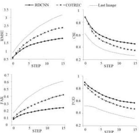
Figure 6. Comparison of four precipitation nowcasting metrics on different models over 15 prediction step.

TABLE I. COMPARISON OF AVERAGE SCORES OF DIFFERENT MODELS OVER 15 PREDICTION STEP.

Model RMSE CSI FAR POD

RDCNN 1.376 0.573 0.187 0.682

COTREC 1.753 0.499 0.292 0.610

Last Image 2.264 0.366 0.444 0.419

Precipitation Nowcasting Metrics Analysis

We evaluate these methods using several commonly used precipitation nowcasting metrics, include rainfall mean squared error (RMSE), critical success index (CSI), false alarm rate (FAR) and probability of detection (POD) [8]. The RMSE metric is defined as the average squared error between the predicted rainfall and the ground truth. Since our predictions are done at the pixel level, we need to convert the image gray scale into radar echo intensities and calculate the precipitation intensity through Z-R relationship [20]. Then we calculate RMSE as follow:

2

0 0

1

RMSE F t( , )x F t( , )x

N   

 





where  is the observation area, N is the total number of pixels, precipitation intensity of the predicted rainfall and the ground truth on pixelx at time step  would be denoted by F t(0, )x and F t(0, )x . Every pixel in prediction and ground truth is marked as 1

or 0 using a threshold of 0.5mm/h rainfall rate (raining or not) when calculating CSI, FAR and POD. Then count the numbers of hits pixels (prediction = 1, truth = 1), misses pixels (prediction = 0, truth = 1) and false pixels (prediction = 1, truth = 0), mark them as nh,nmandnf . CSI, FAR and POD are defined as follow:

CSI h FAR f POD h

h m f h f h m

n

n n

n n n n n n n

  

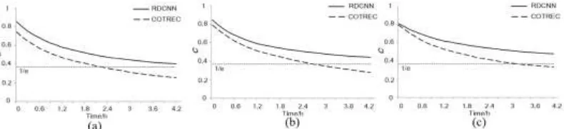
Figure 7. Correlation changes over forecast time during the three precipitation processes. (a) Nanjing on July 11, 2016 (b) Hangzhou on August 20, 2016 (c) Xiamen on July 9, 2016.

We apply the RDCNN and COTREC to predict the precipitation processes in Xiamen, July 9, 2016, and calculate four precipitation nowcasting metrics over 15 prediction steps. In addition, we use the Last Image in thesequence as a reference. Results are shown in Figure 6 and TABLE I. When the forecast time is short, both

RDCNN and COTREC can perform well. While over 5 extrapolated steps, it can be seen that RDCNN outperforms the COTREC algorithm, especially on RMSE and FAR. We infer that the reason RDCNN perform better because it has seen similar patterns during training, it can discover this type of sudden changes and give reasonable predictions in the forecasting.

In this paper, the limitation period of radar echo extrapolation is described by de-correlation time L. It’s related to the correlation between the predicted echo image and the ground truth. The correlation factor cis defined as follow:

0 0

2 2

0 0

( , ) ( , )

( )

( , ) ( , )

G t x G t x c

G t x G t x   

 



 

 



  







Where the gray scale of the pixel x in the prediction and the ground truth at time step  would be denoted by G t(0, )x and G t(0, )x . The time that c drops from 1 to 0 is

defined as the de-correlation time L. Figure 7 shows c changes over forecast time during the three precipitation processes. We can find that the value of c decreases exponentially with the forecast time, compared with COTREC, the correlation factor cof RDCNN decreases more slowly. The results show that L of the COTREC method is approximately 2.4~3 hours, and L of RDCNN is More than 4 hours.

CONCLUSIONS AND FUTURE WORK

For future work, we will investigate how to optimize RDCNN to reduce the fuzzy effect of prediction, and apply RDCNN to video-based action recognition.

REFERENCES

1. Doviak, R. J. 1993. Doppler radar and weather observations, Courier Corporation.

2. Sun, J., Xue, M., Wilson, J. W., Zawadzki, I., Ballard, S. P., and Onvlee-Hooimeyer, J. 2014. “Use of NWP for nowcasting convective precipitation: Recent progress and challenges,” Bulletin of the American Meteorological Society, 95(3), pp. 409-426.

3. Reyniers, M. 2008. “Quantitative precipitation forecasts based on radar observations: Principles, algorithms and operational systems,” Institut. Royal Météorologique de Belgique.

4. Cheung, P., and Yeung, H. Y. 2012. “Application of optical-flow technique to significant convection nowcast for terminal areas in Hong Kong,” In The 3rd WMO International Symposium on Nowcasting and Very Short-Range Forecasting (WSN12), pp. 6-10.

5. Otsuka, S., Tuerhong, G., Kikuchi, R., Kitano, Y., Taniguchi, Y., and Ruiz, J. J. 2016. “Precipitation nowcasting with three-dimensional space–time extrapolation of dense and frequent phased-array weather radar observations,” Weather and Forecasting, 31(1), pp. 329-340.

6. Liang, Q., Feng, Y., Deng, W., Hu, S., Huang, Y., Zeng, Q., and Chen, Z. 2010. “A composite approach of radar echo extrapolation based on TREC vectors in combination with model-predicted winds,” Advances in Atmospheric Sciences, 27(5), pp. 1119-1130.

7. Li, L., Schmid, W., and Joss, J. 1995. “Nowcasting of motion and growth of precipitation with radar over a complex orography,” Journal of applied meteorology, 34(6), pp.1286-1300.

8. Xingjian, S. H. I., Chen, Z., Wang, H., Yeung, D. Y., Wong, W. K., and Woo, W. C. 2015. “Convolutional LSTM network: A machine learning approach for precipitation nowcasting,” In

Advances in neural information processing systems, pp. 802-810.

9. Singh, S., Sarkar, S., and Mitra, P. 2017. “Leveraging Convolutions in Recurrent Neural Networks for Doppler Weather Radar Echo Prediction,” in International Symposium on Neural Networks, pp. 310-317, Springer, Cham.

10. LeCun, Y., Bottou, L., Bengio, Y., and Haffner, P. 1998. “Gradient-based learning applied to document recognition,” Proceedings of the IEEE, 86(11), pp. 2278-2324.

11. Krizhevsky, A., Sutskever, I., and Hinton, G. E. 2012. “Imagenet classification with deep convolutional neural networks,” in Advances in neural information processing systems, pp. 1097-1105.

12. Cireşan, D. C., Giusti, A., Gambardella, L. M., and Schmidhuber, J. 2013. “Mitosis detection in breast cancer histology images with deep neural networks,” In International Conference on Medical Image Computing and Computer-assisted Intervention, pp. 411-418, Springer, Berlin, Heidelberg. 13. Sermanet, P., Eigen, D., Zhang, X., Mathieu, M., Fergus, R., and LeCun, Y. 2013. “Overfeat:

Integrated recognition, localization and detection using convolutional networks,” arXiv preprint arXiv:1312.6229.

14. Yang, W., Jin, L., Tao, D., Xie, Z., and Feng, Z. 2016. “DropSample: A new training method to enhance deep convolutional neural networks for large-scale unconstrained handwritten Chinese character recognition,” Pattern Recognition, 58, pp.190-203.

15. Huang, F. J., and LeCun, Y. 2006. “Large-scale learning with svm and convolutional for generic object categorization,” in Computer Vision and Pattern Recognition, 2006 IEEE Computer Society Conference on , 1, pp. 284-291. IEEE.

16. Mikolov, T., Karafiát, M., Burget, L., Cernocký, J., and Khudanpur, S. 2010. “Recurrent neural network based language model,” in Interspeech, 2, pp. 3.

17. Vinyals, O., Ravuri, S. V., and Povey, D. 2012. “Revisiting recurrent neural networks for robust ASR,” in Acoustics, Speech and Signal Processing (ICASSP), 2012 IEEE International Conference on, pp. 4085-4088. IEEE.

19. Glorot, X., & Bengio, Y. 2010. “Understanding the difficulty of training deep feedforward neural networks.” In Proceedings of the Thirteenth International Conference on Artificial Intelligence and Statistics, pp. 249-256.