Histogram Publishing Method Based on Differential Privacy

2018 International Conference on Computer Science and Software Engineering (CSSE 2018) ISBN: 978-1-60595-555-1

Histogram Publishing Method Based on

Differential Privacy

Xin Liu and Shengen Li

ABSTRACT

Differential privacy does not care about the background knowledge of attackers, and can strongly protect the data information to be released. The distribution of differential privacy histograms based on groupings has drawn much attention from researchers and how to balance the approximation error caused by the group mean with the Laplace error caused by adding noise is the key. This paper proposes a method of APG (Affinity Propagation Clustering and Grouping algorithm) based on clustering grouping to distribute differential privacy histogram, which can effectively balance the approximate error with the Laplace error and improve the histogram posting accuracy. In this method, the index mechanism is used firstly to realize the sorting of the buckets. Then, through the clustering of AP algorithms, the sorted buckets are adaptively grouped to find the optimal grouping strategy and release the data. Experimental results on real data show that APG method is superior to GS, AHP and IHP methods in accuracy of distribution.

INTRODUCTION

The development of science and technology makes life more convenient and produces a large amount of data and information at the same time, such as census information, hospital disease information and bus passenger data information. In order to make full use of these data and information, it is necessary to disclose the data for scientific research planning. For the public data set, while satisfying the data analysis, it is necessary to protect the information of each individual in the data set from being disclosed[1].

_______________________________ Xin Liu, Shengen Li*

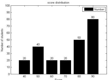
For example, XX class publishes the results of an exam of 230 people in this class. H {40: 20, 50:40, 60:20, 70:20, 80:50, 90:80} As shown in Fig.1, The bucket's result is the bucket's ID. Information attackers can obtain the scores of some of their classmates through the questionnaire. If the attacker now has 200 human data H1 {40:20, 50:30, 60:20, 70:20, 80:50, 90:60}, crossing two data sets

H and H1, the difference obtained by the remaining 30 people, 10 of them score

50 and 20 of 90. If an attacker now has 229 students' information H2, crossover

data sets H and H2, the remaining one's score can be obtained. This attack, which

is based on posting data and obtaining data to cross personal information, is called a differential attack.

In order to prevent attackers differential access to personal privacy data, it is necessary to add "randomness" to the posting data, that is, noise. Post data H '' Add noise to H, H '' = {40:22, 50:39, 60:21, 70:18, 80:48, 90:83}. In this case, personal information cannot be obtained differentially based on the attacker's data H1 and the release data H '', thereby protecting the privacy of the individual[2].

How to balance AE and LE:

1) Consider the global neighborhood of bucket counts. If you sort the buckets from small to large and group them on the sorted result, the approximate error AE is reduced[3]. As shown in Figure 1, the result of each bucket is taken as the bucket ID, the bucket is sorted, the grouping results are {{40,60,70}, {50,80,90}}, and for the grouping of {40,60,70} , Apparently its AE is zero.

2) consider the group leader's question. The longer the packet length, the less noise is added, but the less evenly the bucket counts within the group, the larger the LE[3]. In order to effectively balance the approximation error AE and the Laplace error LE, a histogram distribution method satisfying the clustering groupings of ɛ-differential privacy APG (Affinity Propagation clustering and Grouping algorithm) is implemented in this paper. The method, under the premise of differential privacy, uses an exponential mechanism to sort the histogram and uses AP [4]clustering algorithm to adaptively group.

DEFINITION AND THEORETICAL BASIS

Figure 1. Student Score Distribution Histogram.

Differential Privacy

Given two datasets D and D', histograms H and H' generated by D and D' are in close proximity to each other if they differ from each other by at most one record, ie | D-D'| ≤ 1.

Definition 1[5]. Given an algorithm A, Range (A) is the range of the algorithm A, and for any two H, H' that are mutually adjacent, if the algorithm A arbitrarily outputs the result O(O∈Range(A)) on H and H', The following inequalities are satisfied, A satisfies ɛ- differential privacy.

Pr[A(H)∈O]≤eε×Pr[A(H )′ ∈O] (1)

Among them, the probability Pr depends on the randomness of A; the privacy budget parameter ɛ indicates the degree of privacy protection, the smaller is ɛ, the closer ɛ is to 1, the higher the degree of privacy protection is (0≤ɛ≤1).

Noise Mechanism

The noise mechanism is the main technique to achieve differential privacy protection. The common noise adding mechanisms are the Laplace mechanism[5] and the exponential mechanism[5]. The size of noise added by algorithms based on different noise mechanisms and satisfying differential privacy is closely related to global sensitivity.

Definition 2[5]. The histogram H and H 'of two mutually adjacent relations, any one of the functions f, f : H→Rd, f(H) =(x1, x2, …, xd)T, the global sensitivity

of the function f is:

p H,H

max_′ (H) (H )′

∆ =f f − f (2)

LAPLACE MECHANISM

In the Laplace mechanism, according to the Laplace density distribution function: 2 −ε ∆ ε = ∆ y f

p y e

f | |/

( ) (3)

The probability of a given noise value y.

Theorem 1[5]. For any function f: D → Rd, if the output of Algorithm A satisfies the following inequality, then A satisfies ɛ-differential privacy.

T 1

A(H)=f(H)+ Lap (∆ ε … f/ ), ,Lap (_d ∆ εf/ ) (4) Among them, Lap (_i ∆f / )ε are independent Laplace variables.

INDEX MECHANISM

Theorem 2[5] Given a scoring function u: (H × O) → R, A satisfies ɛ-differential privacy if Algorithm A satisfies the following equation.

u H r

A H u r r O

2 u

 _{ε ∗} 

 = ∈ ∝  ∆    ( , )

( , ) :|Pr[ ] exp( ) (5)

∆u is the global sensitivity of the scoring function. As can be seen from the above equation, the index mechanism uses the scoring function u to score each output, and allocates a greater probability of the index to the output with a higher score, ie, the greater the scoring function, the greater the probability of being selected for output. Scoring functions should have lower sensitivity for better scoring results.

PERFORMANCE MEASUREMENT OF DIFFERENTIAL PRIVACY PROTECTION METHODS

The mean squared error (MSE)[6] is used to measure the effect of posting a histogram H''on response to a set of range count queries [6-26]. Assuming a set of range count queries Q = {Q1, Q2, ..., Qm}, the MSE is calculated as follows:

'' 2

'' 1

(Q (H) Q (H )) MSE(H, H ,Q)

m m i i i= − =

∑

data {H1, H2, ..., Hn} is divided into k groups, and the group is denoted by g, then

the grouping result is expressed as: {g1, g2, ..., gk}, gi = {Hi1, Hi2,..., Hij} . The

approximate error for the i-th packet is:

2 1

AE (H H )

ij

i k i

k i=

=

∑

Theorem 3 [7]. Differential privacy sequence combination: given database D, n random algorithms, A1, A2, ..., An, and Ai (1 ≤ i ≤ n)satisfies ɛ- differential

privacy. {A1, A2, ..., An} The sequence combination on D satisfies ɛ-differential

privacy, and ε=

∑

HISTOGRAM PUBLISHING METHOD UNDER DIFFERENTIAL PRIVACY

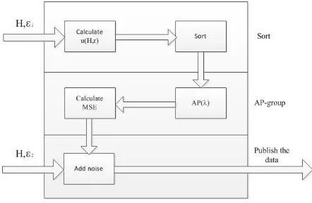
The framework of the APG method in this paper is shown in figure 2. It divides the privacy budget ɛ into two parts, ɛ₁ for sorting and ɛ₂ for adding Laplace noise. The algorithm is divided into three parts:

1)Sort: Enter the original histogram H and the privacy budget ɛ₁, using an exponential mechanism to rank the buckets with similar values as close as possible to approaching the correct order to form the rank H '. Sort index mechanism will consume part of the privacy budget, in improving the accuracy of the data released will be prepared for the next cluster;

2)Grouping: The AP algorithm is adaptive clustering grouping, and does not need to determine the size of the grouping, but different λ values generate different grouping g, calculate MSE under different grouping strategy g according to formula (5), find the best grouping strategy G, Thus improving the accuracy of the final published histogram.

Solve the published histogram: Calculate and publish the final data based on the optimal grouping strategy G and privacy budget ɛ₂.

Sort Method

In order to minimize the approximate error AE, to count the barrel of similar size together, you need to sort according to the bucket count from small to large. When you sort the six buckets in Figure 1, the result of sorting is {H40, H60, H70,

H50, H80, H90}. If you remove one of the H60 buckets, the sorted result becomes

{H60, H40, H70, H50, H80, H90}. The difference between the two data is an

individual, but the output of the sorting results are different, does not satisfy the differential privacy, so the histogram cannot be directly sorted.

This method uses an exponential mechanism to approximate the correct ordering under differential privacy. Theorem 2 shows that under the global privacy of fixed privacy budgets and functions, the core of the exponential mechanism is how to design the scoring function u (Hi, r) (∆u = 1). This design

scoring function consists of two parts:

1) Determine the set of neighbor buckets: Select Hi bucket as the reference to determine the neighbor set Si(Hi) of bucket Hi. Given a distance threshold θ = 2, the set Si (Hi)={Hj:|Hj–Hi| ≤ θ}. The value of θ indicates that the algorithm is a

local ordering. The larger the value of θ is, the more global the ranking is and the global ordering is θ = | H | (θ = | H | / 2 in the experiment).

2) Score each bucket in the neighbor bucket set. Taking the Hi bucket as a benchmark, the scoring function u (H) consists of bucket order and bucket count, that is, u(Hj) = -[ distance(Hj,Hi) + diff_count (Hj,Hi)]. distance(Hj,Hi) refers to

the absolute value of the distance difference between Hj and Hi, diff_count (Hj, Hi)

refers to the absolute value of the difference between Hj and Hi.(The difference in

the count of buckets in the experiment is very large,diff_count(Hj,Hi) =

distance(Hj, Hi)/ max(Hj,Hi), max (Hj, Hi) refers to the maximum count value in

Hj, Hi).

As shown in Fig.1, firstly, a first bucket H40 is selected as a benchmark for

sorting, and S40 = {H50, H60} is the set of neighbor buckets of the H40 bucket

S40(H40)={Hj:|Hj–Hi| ≤2}. u(H50)= -( 1+20) = -21,u(H60) = -(2 +0) = -2,H60

barrels are selected according to exponential mechanism, then the next benchmark is H60 barrels. S60={H50,H70, H80},u(H50)= -21,u(H70)= -1,u(H80)=

-32,then the next benchmark is H70 bucket. S70 = {H50, H80}, then the next

benchmark is H50. H50 neighbor set S50 is empty, then the benchmark at this time

back to the previous benchmark S70 as a benchmark. In this case, S70 = {H80,

H90}, u (H80) = -31, u (H60) = -62, H80 is selected, and finally H90 is selected based

on H80. The final sort result is {H40, H60, H70, H50, H80, H90}.

AP Clustering

the communication between nodes, and divides the other nodes into these centers. AP algorithm has the following advantages:

1)There is no need to determine the number of final clusters. 2) Existing data points as the final cluster center.

Ni represents the i-th data (i∈[ , ]1 n _{) ( N ={ N1, N2, …, Nn}) ,Ci indicates the}

center of clusters in which Ni is clustered(i∈[ , ]1k ，k≤n)，S(Ni, Ci)Represents

the similar measure function of Ni and Ci。When iteratively calculate Ci so that

made

i 1=

∑

min ( , ), Indicating that the clustering is completed.

The similarity measure function of S (Ni, Ci) is implemented by {r (Ni, Ci), a

(Ni, Ci)}, where r (Ni, Ci) Indicates how reliable the ith element data is that Ci is

the cluster center (representing element). a (Ni, Ci) Indicates how much Ci

represents the element's ability to attract Ni. r (Ni, Ci), a (Ni, Ci) Specific formula:

(

) (

)

≠

− +

=

i i i

i i i C s t

i i

C i

C i

r N C S N C a N C s i C

'max { ( , )_{. .} ' ' ( ,

, , )}

(8)

' '

i i i i

' i i . . { N ,C }

( _i, _i) m in {0 , ( _i, _i)} m a x { 0 ,r( ,C )}

N s t N

a N C r C C N

∉

= +

∑

S (i, i) represents the appropriate degree of i as the cluster center of i, and is the

initial value of the AP cluster, that is, the preference. In this paper, we use λ as a

self-clustering factor to adjust the size of Preference, which leads to different grouping strategies. Finally, according to different groupings, we calculate the corresponding MSE and find the most excellent grouping strategy as a group to publish the histogram.

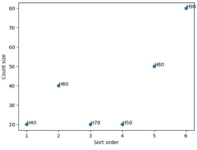
Section 3.2 The ranking results for the data H in Fig.1 are H40 (1,20), H60

(2,20), H70 (3,20), H50 (4,40), H80 (5,50), H90 (6, 80). The scatter plot of the data

is shown in Fig.3. The AP method is used to cluster these six points. The final clustering minimizes the distance between all points and their clustering centers. Suppose we look for the cluster center of H40, initial S (H40, H40) = preference *

λ, and Iteration calculation (H40, c)，a(H40,c) (c= H40, H50,…, H90). When the

cluster center no longer changes, c is the cluster center of H40. The final

clustering result is: {{H40, H60, H70} 1, {H50, H80} 2, {H90} 3}.

The privacy budget is set to 0.5 and Laplacian noise {22.3, 21.8, 22.8, 23.4, 22.1, 21.9} is directly added to the data H {20, 40, 20, 20, 50, 70},The result is

H1 ’’={42.3, 61.8, 42.8, 43.4, 72.1, 91.9}.

mean for group 3 is: {80}. According to the Laplace mechanism, the noise produced by group 3 is {22} and the final group 3 is {102}. Data H = {20, 40, 20,

20, 50, 80} is finally released by the APG algorithm H2'' = {26.1, 54.8, 26.5, 27,

53.9, 102}.

Calculate MSE according to formula (6). For calculation convenience, let Q be the unit length query (that is, query the count of one bucket). Calculated as follows:

MSE(H,H1ʹʹ) = ( (42.3-20)2 +(61.8-40)2 +(42.8-20)2 +(43.4-20)2

+(72.1-50)2+(91.9-80)2 ) /6 =501.

MSE(H,H2ʹʹ) = ( (26.1-20)2 +(54.8-40)2 +(26.5-20)2 +(27-20)2 +(53.9-50)2

+(102-80)2 ) /6 =141.

Based on the above calculation results, it is clear that adding noise to the data after sorting the packets will reduce the MSE, which further verifies the practicability of the packet technology.

EXPERIMENTAL RESULTS AND ANALYSIS

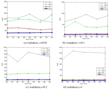
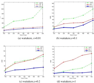
The experiment used two data sets waitakere[9], social_network. Waitakere is the population census data of New Zealand in 2006, taking 7725 block data. social_network is internet data, for a total of 11324 data records. These two data sets are widely used for histogram information dissemination.

By comparing the number of range queries, size and different privacy budgets to compare the accuracy of the results of different methods in the corresponding range queries, the availability of histograms published by different methods is compared. On both data sets, the mean square error MSE was used to measure the accuracy and availability of the histograms published by the IHP, AHP, GS, and

APG methods in this article by setting the privacy budget ɛ = 0.01, 0.1, 0.2, 1.

When solving MSE, the length of the query is set randomly. As the number of queries increases, the value of MSE tends to be stable. The experimental horizontal axis indicates the number of experiments. From the experimental results, it can be found that the Laplacian error added will decrease and the error

of MSE will be reduced when ɛ gradually increases from 0.01 to 1. As shown in

Figure 4 (a-d) and Fig.5 (a-d). When ɛ = 1, the error in this case is only composed

of approximate errors, and the value of MSE will not be equal to zero, as shown in Fig.4 (d) and 5 (d). According to the experimental results in Fig.4 and Fig.5, it is found that the APG method is more accurate than the other methods under different data sets and privacy budgets. First of all, for the IHP [10] method, Laplacian noise is increased for data with uneven distribution of barrel counts in the histogram. For AHP [11], sorting the noisy data grouping reduces the availability of the published data. For GS [13], fixed packet size, to a large extent, will increase the approximate error.

Waitakere data under different privacy budget experimental results:

(a) waitakere, ɛ=0.01 (b) waitakere, ɛ=0.1

(c) waitakere,ɛ=0.2 (d) waitakere,ɛ=1

(a) social_network,ɛ=0.01 (b) social_network,ɛ=0.1

(c) social_network,ɛ=0.2 (d) social_network,ɛ=1

Figure 5. social_network data, MSE with the number of changes in the query.

(a) waitakere, ɛ=0.01 (b) waitakere,ɛ=0.1

(c) waitakere,ɛ=0.2 (d) waitakere,ɛ=1

According to the comparison of the MSE sizes of the above four algorithms, the availability of the GS algorithm is lower. In the following MSE and query scope relationship comparison, the GS method is no longer discussed. Change the scope of the query and the size of the privacy budget to compare the accuracy of the results of AHP, IHP and APG methods in the corresponding range query. As can be seen from the four graphs (a), (b), (c) and (d) of Fig. 6, the error increases as the privacy budget increases. As the range of queries increases, the value of MSE increases. This is because as the scope of the query increases, the Laplacian

noise will be accumulated[6]. As can be seen from Fig.6 (a), (b) and (c), the

larger the privacy budget, the smaller the error of releasing the data. When the privacy budget is 1, Laplacian noise is not added at this time, and the data error is only approximate error, as shown in Fig.6(d).

CONCLUSION

Aiming at the issue of packet-based histogram distribution under differential privacy, this paper proposes clustering-based grouping method APG, which uses the exponential mechanism to gradually approximate the correct ordering of buckets.The clustering algorithm is used to group the sorted buckets adaptively, and the approximate error and Laplace error are balanced. From the theoretical and experimental standpoints, this method is proved to be more practical than other methods in satisfying differential privacy. Future work is prepared to consider data dissemination of spatial data based on differential privacy.

ACKNOWLEDGMENTS

This work was financially Supported by the National Natural Science Foundation of China (61170052)

REFERENCES

1. Homer N, Szelinger S, Redman M, et al. Resolving individuals contributing trace amounts of DNA to highly complex mixtures using high-density SNP genotyping micro- arrays.[J]. Plos Genetics, 2008, 4(8):e1000167.

2. Mcsherry F, Talwar K. Mechanism Design via Differential Privacy[C]//Foundations of Computer Science, 2007. FOCS '07. IEEE Symposium on. IEEE, 2007:94-103.

3. Dwork C, Roth A. The Algorithmic Foundations of Differential Privacy[M]. Now Publishers Inc. 2014.

4. Wang K, Zhang J, Dan L, et al. Adaptive Affinity Propagation Clustering[J]. Acta Automatica Sinica, 2007, 33(12):1242-1246.

6. Zhang Xiaojian, Shao Chao, Meng Xiaofeng. An accurate histogram distribution method for differential privacy[J]. Journal of Computer Research and Development. , 2014(4):927-949.

7. Zhang XiaoJian, Shao chao, Meng XiaoFeng. Differential Privacy A precise histogram distribution method[J]. Computer Research and Development, 2016, 53(5):1106-1117. 8. Zhang XiaoJian, Meng XiaoFeng. Stream Histogram Publishing Method Based on

Differential Privacy[J]. Software Journal, 2016, 27(2):381-393.

9. Li H, Cui J, Lin X, et al. Improving the utility in differential private histogram publishing: Theoretical study and practice[C]// IEEE International Conference on Big Data. IEEE, 2017:1100-1109.

10. Kellaris G, Papadopoulos S. Practical differential privacy via grouping and sWang K, Zhang J, Dan L, et al. Adaptive Affinity Propagation Clustering[J]. Acta Automatica Sinica, 2007, 33(12): 1242-1246.

11. Zhang X, Chen R, Xu J, et al. Towards Accurate Histogram Publication under Differential Privacy[M]// Proceedings of the 2014 SIAM International Conference on Data Mining. 2014.

12. Chao Li, Michael Hay, Gerome Miklau, et al. A Data- and Workload-Aware Algorithm for Range Queries Under Differential Privacy[J]. Proceedings of the Vldb Endowment, 2014, 7(5).

13. moothing[C]// International Conference on Very Large Data Bases. VLDB Endowment, 2013:301- 312.

14. Machanavajjhala A, He X, Hay M. Differential Privacy in the Wild: A Tutorial on Current Practices & Open Challenges[J]. Proceedings of the Vldb Endowment, 2016, 9(13): 1611-1614.

15. Lin C, Wang P, Song H, et al. A differential privacy protection scheme for sensitive big data in body sensor net- works[J]. Annals of Telecommunications, 2016, 71(9-10): 465-475. 16. Xiao X, Bender G, Hay M, et al. iReduct:differential privacy with reduced relative

errors[C]//ACM SIGMOD International Conference on Management of Data, SIG- MOD 2011, Athens, Greece, June. DBLP, 2011:229-240.

17. Li, Yang D, Zhang, et al. Compressive mechanism: utilizing sparse representation in differential privacy[J]. 2011:177-182.

18. Xiao X, Wang G, Gehrke J. Differential Privacy via Wavelet Transforms[J]. IEEE Transactions on Knowledge & Data Engineering, 2011, 23(8):1200-1214.

19. Hardt M, Talwar K. On the geometry of differential privacy[C]// ACM Symposium on Theory of Computing. ACM, 2010:705-714.

20. Hay M, Rastogi V, Miklau G, et al. Boosting the accuracy of differentially private histograms through consistency[J]. Proceedings of the Vldb Endowment, 2010, 3(1-2):1021-1032.

21. Li N, Qardaji W, Dong S. On sampling, anonymization, and differential privacy or, k-anonymization meets differential privacy[J]. 2011, abs/1101.2604:32-33.

22. Acs G, Castelluccia C, Chen R. Differentially Private Histogram Publishing through Lossy Compression[C]//IEEE, International Conference on Data Mining. IEEE, 2013:1- 10. 23. Zhang Z, Zhang Z, Winslett M, et al. Low-rank mechanism: optimizing batch queries under

differential privacy[J]. Pro- ceedings of the Vldb Endowment, 2012, 5(11):1352- 1363. 24. Li C, Miklau G, Hay M, et al. The matrix mechanism: optimizing linear counting queries

under differential privacy[J]. Vldb Journal, 2015, 24(6):757-781.

25. Song, Chunyao, Ge, Tingjian. Aroma: A New Data Protection Method with Differential Privacy and Accurate Query Answering[J]. 2014:1569-1578.