New inertial algorithm for solving split common null point problem in Banach spaces

R E S E A R C H

Open Access

New inertial algorithm for solving split

common null point problem in Banach spaces

Yan Tang

*_{Correspondence:} [email protected] 1_{College of Mathematics and} Statistics, Chongqing Technology and Business University, Chongqing, China

Abstract

Inspired by the works of Alvarez and Attouch (Set-Valued Anal. 9:3–11,2001), López et al. (Inverse Probl. 28:ID085004,2012), Takahashi (Arch. Math. (Basel) 104(4):357–365, 2015) and Suantai et al. (Appl. Gen. Topol. 18(2):345–360,2017), as well as Promluang and Kuman (J. Inform. Math. Sci. 9(1):27–44,2017), we propose a new inertial algorithm for solving split common null point problem without the prior knowledge of the operator norms in Banach spaces. Under mild and standard conditions, the weak and strong convergence theorems of the proposed algorithms are obtained. Also the split minimization problem is considered as the application of our results. Finally, the performances and computational examples are presented, and a comparison with related algorithms is provided to illustrate the efficiency and applicability of our new algorithm.

MSC: 47H05; 47H09; 49J53; 65J15; 90C25

Keywords: Split common null point problem; Inertial technique; Self-adaptive step size; Set-valued; Strong convergence

1 Introduction

In an excellent paper [6], Byrne, Censor, Gibali and Reich introduced the following split common null point problem (SCNPP) for set-valued operators: find a pointx∗∈H1such

that

0∈ p

i=1

Aix∗, (1.1)

and

y∗_j =Tjx∗∈H2 such that 0∈Bj

y∗_j, for eachj= 1, 2, . . . ,r, (1.2)

whereH1andH2are two real Hilbert spaces andAi:H1→2H1,Bj:H2→2H2are maximal

monotone operators,Tj:H1→H2are bounded linear operators.

The split common null point problem is motivated by many related problems. The first is the split inverse problem (SIP) which is formulated in Censor, Gibali and Reich [7]. It concerns a model in which two vector spacesXandY and a linear operatorA:X→Y

are given. In addition, two inverse problems are involved. The first one, denoted byIP1,

is formulated in the space X, and the second one, denoted byIP2, is formulated in the

spaceY. Given these data, the SIP is formulated as follows:

find a pointx∗∈Xthat solvesIP1

and such that

the pointy=Tx∗∈YsolvesIP2.

The first instance of SIP is the split convex feasibility problem (SCFP) (see, e.g., Censor and Elfving [8]) in whichIP1andIP2are the convex feasibility problems (CFP). The SCFP

has been well studied during the last two decades, both theoretically and practically. In particular, the CFP has been used to model significant real-world problem in sensor net-work, radiation therapy treatment planning, resolution enhancement, and in many other instances; see, e.g., Byrne [9] and the references therein.

Soon after, many authors asked if other inverse problems can be used forIP1andIP2,

besides CFP, and be embedded in the SIP methodology. For example, can SIP be with a Null Point Problem in each of the two spaces?

In fact, the SCNPP can be put in the context of SIP and related works. For instance, the split variational inclusion problem (SVIP) which is an SIP with VIP in each of the two spaces (see, e.g., Censor et al. [7]). The SVIP is formulated as follows:

find a pointx∗∈Csuch thatfx∗,x–x∗≥0 for allx∈C, and such that

the pointy∗=Tx∗∈Qand solvesgy∗,y–y∗≥0 for ally∈Q,

whereCandQare nonempty closed convex subsets of Hilbert spacesH1andH2,

respec-tively,f :H1→H1 andg:H2→H2 are two given operators,T:H1→H2 is a bounded

linear operator. If we takeC=H1,Q=H2 andx=x∗–f(x∗),y=y∗–g(y∗) in SVIP, then

we can get the split zero problem (SZP) which is introduced in Censor et al. [7] (Sect. 7.3). The formulation of SZP is as follows:

find a pointx∗∈H1

such thatfx∗= 0 andgTx∗= 0.

Following the idea in Censor et al. [7] and Rockafellar [10], Moudafi [11] introduced the split monotone variational inclusion (SMVI) which generalized the SVIP. The SMVI is as follows:

find a pointx∗∈H1such that 0∈f

x∗+B1

x∗

and such that the point

y∗=Tx∗∈H2and solves 0∈g

y∗+B2

y∗,

to see that the SZP is obtained from SMVI by lettingB1andB2be zero operators. Since in

Moudafi [11] all the applications of the SMVI were presented forf =g= 0, it follows that these applications are also covered by the SCNPP. In addition, the SCNPP is a generation of SZP.

Consequently, the SCNPP (1.1)–(1.2) has attracted wide attention thanks to the motiva-tion of the above related problems and works. As for its applicamotiva-tions in signal processing and image reconstruction, the reader can refer to Ansari and Rehan [12,13], Censor et al. [14], Ceng et al. [15] and the reference therein.

Under the idea ofCQalgorithm in Byrne [16,17], relaxedCQalgorithm in Yang [18], extra-gradient method in Ceng et al. [15], many authors were dedicated to the study of the approximation solution of the SCNPP (1.1)–(1.2) for two set-valued mappings in Hilbert spaces in recent years, for instance, Byrne et al. [6] studied the following iterative method for two set-valued maximal operators in Hilbert spaces:

xn+1=JλA

xn+γT∗

JλB–I

Txn

, ∀n≥1,∃λ> 0, (1.3)

and obtained weak convergence of the sequence under suitable conditions. For more de-tails on the methods of solving the SCNPP and the related issues in Hilbert spaces, the reader might refer to Moudafi and Thakur [19], Gibali et al. [20], Censor et al. [7], Shehu and Iyiola [21], Ceng et al. [22], Sitthithakerngkiet et al. [23].

Based on the above works, Takahashi [3,24] extended such a problem in Hilbert spaces to Banach spaces and then obtained strong convergence theorems. Soon afterwards, Alofi, Alsulami and Takahashi [25] introduced the following Halpern’s iteration to find a com-mon solution of split null point problem between Hilbert and Banach spaces:

xn+1=βnxn+ (1 –βn)(αnun+ (1 –αn)JλAn

xn+λnT∗JE

QBμ–I

Txn

, ∀n≥1, (1.4)

whereJEis duality mapping on a Banach space,{un}is a sequence in a Hilbert space such thatun→u, and the step sizeλnsatisfies 0 <λnT2< 2. Under suitable assumptions, they obtained a strong convergence theorem. Very recently, Suantai et al. [4] proposed the following scheme to approximate the solution of SCNPP for two set-valued mappings in Banach spaces:

xn+1=αnf(xn) +βnxn+γnJλAn

xn+λnT∗JE

QBμ–I

Txn

, ∀n≥1, (1.5)

where the step size satisfies 0 <λnT2< 2. For more works on the solution of the SCNPP for two set-valued mappings in Banach spaces and related issues, the reader might refer to Promluang and Kuman [5], Kamimura and Takahashi [26], Takahashi [27], Ansari and Rehan [28], Kazmi and Rizvi [29], among others.

On the other hand, López [2] presented an algorithm in Hilbert spaces for solving split feasibility problem whose step size is self-adaptive:

xk+1=PCk

I–τkT∗(I–PQk)T

xn, ∀k≥1,

where the step sizeτk=_∇ρk_ff_(x(x_k)k)2,f(xk) =

(I–P_Qk)Txn

2 ,∇f(xk) =T∗(I–PQk)Txn.

In addition, for approximating the null point of a maximal monotone operator, Alvarez and Attouch [1] introduced the following inertial proximal algorithm:

xn+1=JλAn

xn+αn(xn–xn–1)

, ∀n≥1,

and obtained the weak convergence of the algorithm. Roughly speaking, the inertial tech-nique may be exploited in some situations in order to “accelerate” the convergence. This point of view inspired various numerical methods related to the inertial terminology, all of them have nice convergence properties by incorporating second order information, see, e.g., Mainge [30], Alvarez [31,32].

So it is natural to ask the following question:

Question 1.1 Can we construct a new inertial algorithm for solving the SCNPP (1.1)– (1.2) for two set-valued mappings in Banach spaces without prior knowledge of the oper-ator normT?

Motivated and inspired by the works of Alvarez and Attouch [1], Gibali et al. [20], López et al. [2], Takahashi [3], Alofi et al. [25] and Suantai et al. [4], as well as Promluang and Kuman [5], we wish to provide an affirmative answer to this question. Our contribution is a new inertial method, combining the idea of inertial proximal technique with self-adaptive rule, for solving the solution of the split common null point problem (SCNPP) (1.1)–(1.2) for two set-valued mappings in Banach spaces.

The outline of the paper is as follows. In Sect.2, we collect definitions and results which are needed for our further analysis. In Sect.3, our new inertial algorithms in Banach spaces are introduced and analyzed, and the weak and strong convergence theorems are obtained. In addition, the split minimizing problem is introduced as the application of our results in Sect.4. Finally, numerical experiment including compressed sensing and a comparison with related algorithms are provided to illustrate the performances of our new algorithms.

2 Preliminaries

LetEbe a real Banach space with norm·and letE∗be the dual space ofE. A normalized duality mappingJ:E→2E∗_{is defined by}

Jx=x∗∈E∗:x,x∗=x∗2=x2 ,

where·,·denotes generalized duality pairing betweenEandE∗. LetU={x∈E:x= 1}. The norm ofEis said to be Gâteaux differentiable if for eachx,y∈U, the limit

lim t→0

exists. In the case,Eis called smooth. It is well known thatEis smooth if and only ifJ

is single-valued and ifEis uniformly smooth thenJis uniformly continuous on bounded subsets ofE. We note that in a Hilbert space,Jis the identity operator.

A Banach spaceEis said to bep-uniformly smooth if for a fixed real number 1 <p≤2, there exists a constantc> 0 such thatρ(t) =ctp_{for allt> 0. From Chang et al. [33] and} Chidume [34], we know that ifEis a 2-uniformly smooth Banach space, then for allx,y∈E

there exists a constantc> 0 such thatJx–Jy ≤cx–y.

A multi-valued mappingA:E→2E∗_{with domainD(A) ={x∈E,Ax=∅}is said to be} monotone if

x–y,x∗–y∗≥0,

for allx,y∈D(A),x∗∈Axandy∗∈Ay. A monotone operatorAonEis said to be maximal if its graph is not properly contained in the graph of any other monotone operator onE. The following theorem is due to Browder [35], see also Takahashi [36].

Theorem 2.1(Browder [35]) Let E be a uniformly convex and smooth Banach space,and let J be the duality mapping of E into E∗.Let A be a monotone operator of E into2E∗_.Then

A is maximal if and only if for any r> 0,

R(J+rA) =E∗,

whereR(J+rA)is the range of J+rA.

LetEbe a uniformly convex Banach space with a Gâteaux differentiable norm, and let

A:E→2E∗_{be a maximal monotone operator. Now we consider the metric resolvent ofA}

QAμ=

I+μJ–1A–1, μ> 0. It is well known that the operatorQA

μis firmly nonexpansive and the fixed points of the op-eratorQAμare the null points ofA; see, e.g., Kohsaka and Takahashi [37,38]. The resolvent plays an essential role in the approximation theory for zero points of maximal monotone operators in Banach spaces. According to the work of Aoyama et al. [39], we have the following properties:

QAμzn–y,J

zn–QAμzn

≥0, y∈A–1(0), (2.1)

in particular, ifEis a real Hilbert space, then

JμAzn–y,zn–JμAzn

≥0, y∈A–1(0), (2.2)

whereJA

μ = (I+μA)–1is the general resolvent,A–1(0) ={z∈E: 0∈Az}. For more details on the properties of firmly nonexpansive mappings, one can see, e.g., Aoyama et al. [39], Bauschke et al. [40].

is,

ww(xn) :=x∈H:xnjxfor some subsequence{nj}of{n} .

It is well known that

αx+βy+γz2=αx2+βy2+γz2

–αβx–y2–βγy–z2–γ αx–z2, (2.3)

for anyx,y,z∈Hand for allα,β,γ withα+β+γ = 1. Moreover, the following inequality holds:

x+y2≤ x2+ 2y,x+y, ∀x,y∈H. (2.4)

LetCbe a closed convex subset ofH. For every elementx∈H, there exists a unique nearest point inC, denoted byPCx, such that

x–PCx=min

x–y:y∈C .

The operatorPCis called the metric projection ofHontoCand some of its properties are summarized as follows:

x–y,PCx–PCy ≥ PCx–PCy2, ∀x,y∈H.

Moreover, for allx∈Handy∈C,PCxis characterized by

x–PCx,y–PCx ≤0. (2.5)

Lemma 2.2(see, e.g., Xu [41] and Maingé [42]) Assume that{an}is a sequence of

nonneg-ative real numbers such that

an+1≤(1 –θn)an+δn, n≥0,

where{θn}is a sequence in(0, 1)and{δn}is a sequence such that (1) ∞_n=1θn=∞;

(2) lim sup_n→∞δn

θn≤0or

_∞

n=1|δn|<∞.

Then the sequence{an}has a limit andlimn→∞an= 0.

Lemma 2.3(see, e.g., Maingé [43]) Let{Γn}be a sequence of real numbers that does not

decrease at infinity,in the sense that there exists a subsequence{Γnj} of{Γn} such that

Γnj<Γnj+1for all j≥0.Also consider the sequence of integers{σ(n)}n≥n0 defined by

σ(n) =max{k≤n:Γk≤Γk+1}.

Then{σ(n)}n≥n0is a nondecreasing sequence verifyinglimn→∞σ(n) =∞and,for all n≥n0,

Lemma 2.4(see, e.g., Halpern [44] and Suzuki [40]) Let H be a real Hilbert space and

{xn} ∈H such that there exists a nonempty closed convex subset C⊂H satisfying (i) For everyz∈C,limn→∞xn–zexists;

(ii) Any weak cluster point of{xn}belongs toC.

Then there existsx¯∈C such that{xn}converges weakly tox¯.

Lemma 2.5(see, e.g., Maingé [30]) Let{Γk}and{δn}be sequences in[0, +∞)which satisfy: (i) Γn+1–Γn≤θn(Γn–Γn–1) +δn;

(ii) ∞_n=1δn<∞;

(iii) θn∈[0,θ],whereθ∈[0, 1).

Then{Γn}is a converging sequence and

_∞

n=1[Γn+1–Γn]+<∞,where[t]+=max{t, 0}for any t∈R.

3 Main results

In this section, we introduce our algorithms and state our main results.

Throughout the rest of this paper, we always assume thatHis a real Hilbert space and

E is a 2-uniformly convex smooth Banach space. Let A:H→2H, B:E→2E∗ be two maximal monotone operators. LetT :H→Ebe a bounded linear operator with adjoint operatorT∗:E∗→HandT=∅.

Consider the following split common null point problem in Banach spaces:

findx∗∈Hsuch that 0∈Ax∗

andy∗=Tx∗∈Esuch that 0∈By∗.

Now we define the functions

f(xn) =1 2J

I–QBμ

Txn

2

, h(xn) =1 2I–J

A r

xn

2

,

and

F(xn) =T∗JI–QBμ

Txn, H(xn) =I–J_rAxn,

whereJis the duality operator onE.

In the rest of this paper, we denoteΩ=A–1_(0)∩T–1_(B–1_{0), which meansΩ={x}∗_∈H: x∗∈A–1(0),Tx∗∈B–1(0)}.

3.1 Algorithms

Algorithm 3.1 Choose two positive sequences {n}, {ρn} satisfying

∞

n=1n < ∞, 0 <ρn< 4.

Select arbitrary starting pointsx0,x1∈C, constantα∈[0, 1), and chooseαnsuch that 0 <αn<α¯n, where

¯ αn=

⎧ ⎨ ⎩

min{α,n(max{xn–xn–12,xn–xn–1})–1}, xn=xn–1,

Iterative Step.Given the iteratesxn(n≥1), forr> 0, compute

wn=xn+αn(xn–xn–1), (3.1)

and calculate the step size

λn=ρn

f(wn) F(wn)2+H(wn)2

,

and the next iterate

xn+1=JrA

I–λnT∗J

I–QBμ

Twn. (3.2)

Stop Criterion.Ifxn+1=wnthen stop. Otherwise, setn:=n+ 1 and return to Iterative Step.

Algorithm 3.2 Choose positive sequences{n},{ρn},{βn}and{γn}satisfying

∞

n=1n< ∞, 0 <ρn< 4 and

0 <βn,γn< 1, infβn(1 –βn–γn) > 0, ∀n∈N;

lim n→∞γn= 0,

∞

n=1

γn=∞, n=o(γn).

Select arbitrary starting pointsx0,x1∈C, constantα∈[0, 1), and chooseαnsuch that 0 <αn<α¯n, where

¯ αn=

⎧ ⎨ ⎩

min{α,n(max{xn–xn–12,xn–xn–1})–1}, xn=xn–1,

α, otherwise.

Iterative Step.Given the iteratesxn(n≥1), forr> 0,μ> 0, compute

wn=xn+αn(xn–xn–1),

and calculate the step size

λn=ρn

f(wn)

F(wn)2_+H(wn)2,

and the next iterate

xn+1= (1 –βn–γn)wn+βnJrA

I–λnT∗J

I–QBμ

Twn. (3.3)

3.2 Weak convergence analysis for Algorithm3.1

Lemma 3.1 Let H be a real Hilbert space,E a strictly convex reflexive and smooth Banach

space,and let J be duality mapping on E.Let A:H→2H,B:E→2E∗be maximal operators such that A–1_{(0)=∅and B}–1_{(0)=∅.Let T:H→E be a bounded linear operator such that} T=∅and T∗be the adjoint operator of T.Suppose thatΩ=A–1(0)∩T–1(B–1(0))=∅.Let

λ,μ,r> 0and z∈H.Then the following are equivalent: (1) z∈A–1_(0)∩T–1_(B–1_(0));

(2) z=J_rA(I–λT∗J(I–QBμ)T)z,

where JA

r = (I+rA)–1,QμB= (I+μJ–1B)–1.

Proof SinceA–1(0)∩T–1(B–1(0))=∅, there existsz0∈A–1(0) such thatTz0∈B–1(0).

(2)⇒(1). Assumingz=JA

r(I–λT∗J(I–QBμ)T)z, it follows from property (2.2) ofJrAthat

z–λT∗JTz–QBμTz

–z,z–y≥0, ∀y∈A–1(0),

which yields

–λT∗JTz–QB_μTz,z–y≥0, ∀y∈A–1(0),

and hence

T∗JTz–QBμTz

,z–y≤0, ∀y∈A–1(0).

Therefore

JTz–QB_μTz,Tz–Tz0

≤0. (3.4)

On the other hand, sinceQB

μis the resolvent ofBforμ> 0, we have

JTz–QBμTz

,QBμTz–v

≥0, v∈B–1(0).

It follows fromTz0∈B–1(0) that

JTz–QBμTz

,QBμTz–Tz0

≥0. (3.5)

Combining with (3.4) and (3.5), we can get

JTz–QBμTz

,Tz–QBμTz

≤0,

that is,

QBμTz–Tz

2

≤0,

which means thatQB

(1)⇒(2). Sincez∈A–1_(0)∩T–1_(B–1_{(0)), we have thatTz∈B}–1_{(0) and z∈A}–1_{(0). It}

follows thatz=JA

rzandTz=QBμTz. Thus we get

J_rAI–λT∗JI–QBμ

Tz=J_rAz=z.

This completes the proof.

Lemma 3.2 Let H be a real Hilbert space,E a real2-uniformly smooth Banach space,and let J be duality mapping on E.Let A:H→2H_,B:E→2E∗ _{be maximal operators such}

that A–1(0)=∅and B–1(0)=∅.Let T:H→E be a bounded linear operator with adjoint operator T∗:E∗→H and T=∅.Assume that T–1_(B–1_{(0))=∅.Let F=T}∗_J(I–QB

μ)T,then

F is Lipschitz continuous.

Proof According to the work of Kohsaka and Takahashi [37, 38], QB

μ is nonexpansive. Moreover, sinceE is a 2-uniformly smooth Banach space, there exists a constantc> 0 such thatJx–Jy ≤cx–yfor allx,y∈E, therefore we estimate

Fx–Fy=T∗JI–QBμ

Tx–T∗JI–QBμ

Ty

=T∗JI–QBμ

Tx–JI–QBμ

Ty

≤T∗JI–QBμ

Tx–JI–QBμ

Ty) ≤cT∗I–QB_μTx–I–QB_μTy) ≤cT∗(Tx–Ty+QBμTx–QBμTy ≤2cT2x–y,

which implies thatFis Lipschitz continuous. Similarly,I–JA

r is Lipschitz continuous. This

completes the proof.

Lemma 3.3 Let us consider the split common null point problem with its solutionΩ=

A–1_(0)∩T–1_(B–1_{0)in Banach spaces.If x}

n+1=wnin Algorithm3.1,then wn∈Ω.

Proof Ifxn+1=wn, then we havewn=JrA(I–λnT∗J(I–QBμ)T)wn. According to Lemma3.1, we conclude thatwn∈A–1(0) andTwn∈B–1(0), that is,wn∈Ω. The proof is complete.

Theorem 3.4 Let H be a real Hilbert space,E be a uniformly convex and2-uniformly

smooth Banach space.Let A:H→2H,B:E→2E∗be two maximal monotone operators such thatΩ=A–1_(0)∩T–1_(B–1_{0)=∅.Let T:H→E be a bounded linear operator with} ad-joint operator T∗:E∗→H and T=∅.Then the sequence{xn}generated by Algorithm3.1

converges weakly to x∗∈Ω.

Proof Without loss of generality, we takez∈Ω, and then getz=JA

rz, Tz=QBμTzand

J_rA(I–λnT∗J(I–QBμ)T)z=z, therefore from (2.3) we obtain

wn–z2 =xn+αn(xn–xn–1) 2

≤(1 +αn)xn–z2–αnxn–1–z2+αn(1 +αn)xn–xn–12

≤(1 +αn)xn–z2–αnxn–1–z2+ 2αnxn–xn–12, (3.6)

and sinceJA

r is nonexpansive,

xn+1–z2 =JrA

I–λnT∗J

I–QBμ

Twn–z2 ≤I–λnT∗J

I–QB_μTwn–z

2

=wn–z2– 2λn

wn–z,T∗J

I–QB_μTwn

+λ2_nT∗JI–QB_μT)wn

2

=wn–z2– 2λn

Twn–Tz,J

I–QB_μTwn

+λ2_nF(wn)

2

.

It follows from property (2.1) ofQBμthat

QBμTwn–Tz,J

Twn–QBμTwn

≥0, Tz∈B–1(0),

and then we have that

Twn–Tz,J

I–QBμ

Twn

=Twn–QBμTwn,J

Twn–QBμTwn

+QBμTwn–Tz,J

Twn–QBμTwn

=Twn–QBμTwn2+

QBμTwn–Tz,J

Twn–QBμTwn

≥JTwn–QBμTwn2 = 2f(wn).

Therefore we have from (3.6) that

xn+1–z2≤ wn–z2– 4λnf(wn) +λ2nF(wn)

2

≤(1 +αn)xn–z2–αnxn–1–z2+ 2αnxn–xn–12

+ ρ

2

nf2(wn) (F(wn)2+H(wn)2)2

F(wn)2– 4 ρnf

2_(wn)

F(wn)2+H(wn)2 ≤(1 +αn)xn–z2–αnxn–1–z2+ 2αnxn–xn–12

+ (ρn– 4)

ρnf2(wn)

F(wn)2_+H(wn)2. (3.7)

Thus we get

xn+1–z2–xn–z2≤αn

xn–z2–xn–1–z2

+ 2αnxn–xn–12

+ (ρn– 4)

ρnf2(wn) F(wn)2_+H(wn)2

≤αn

xn–z2–xn–1–z2

and

(4 –ρn)

ρnf2(wn) F(wn)2_+H(wn)2

≤ xn–z2–xn+1–z2+αn

xn–z2–xn–1–z2

+ 2αnxn–xn–12. (3.9)

The fact that

αnxn–xn–12≤ ¯αnxn–xn–12≤n

implies∞_n=1αnxn–xn–12<

∞

n=1n<∞. DenotingΓn=xn–z2and using Lemma2.5 in (3.8), we conclude thatxn–z2is a converging sequence, which implies that{xn}is bounded, and so is{wn}.

Moreover, we have∞_n=1(xn–z2–xn–1–z2)+<∞, and it follows from (3.9) that f2_(w

n)

F(wn)2_+H(wn)2 →0.

SinceF(wn) andH(wn) are Lipschitz continuous by Lemma3.2, they are bounded, thus we havef(wn)→0, therefore

JTwn–QBμTwn

2

=Twn–QBμTwn→0. (3.10)

Next we show thatwwn(xn)⊂Ω. Letx¯∈wwn(xn) be an arbitrary element. Since{xn}is bounded, there exists a subsequence{xnk}of{xn}which converges weakly tox¯. Note that again

αnxn–xn–1 ≤ ¯αnxn–xn–1 ≤n→0,

which implies thatwn–xn=αnxn–xn–1 →0. Therefore, there exists a subsequence

{wnk} of{wn}which converges weakly tox¯. It follows from the lower semicontinuity of (I–QB

μ)TandJthat

Tx¯–QBμTx¯= lim k→∞inf

Twnk–QBμTwnk= 0,

which means thatTx¯∈B–1_(0).

On the other hand, according (2.4), we have

xn+1–wn2 =xn+1–z–wn+z2

≤ wn–z2–xn+1–z2+ 2xn+1–wn,xn+1–z

≤(1 +αn)xn–z2–αnxn–1–z2+ 2αnxn–xn–12–xn+1–z2

+ 2xn+1–wn,xn+1–z

=xn–z2–xn+1–z2+αn

xn–z2–xn–1–z2

According to property (2.2) of the resolvent, we haveJA

rzn–z, (I–λnT∗J(I–QBμ)T)wn–

xn+1 ≥0, wherezn= (I–λnT∗J(I–QBμ)T)wn,xn+1=JrAzn andz∈A–1(0). Therefore, it follows from (3.10) that

xn+1–z,xn+1–wn ≤

xn+1–z, –λnT∗J

Twn–QBμTwn

→0.

Thus, it follows from (3.11) thatxn+1–wn →0, which yieldsJrA(I–λnT∗J(I–QBμ)T)wn–

wn →0. Since recursion (3.3) can be rewritten aswn–xn+1–λnT∗J(I–QBμ)Twn∈rAxn+1,

we can conclude that

1

r

wn–xn+1–λnT∗J

I–QB_μTwn

∈Axn+1.

In addition, from (3.10) and (3.11), we get that

wn–xn+1–λnT∗J

I–QBμ

Twn≤ wn–xn+1+λnT∗J

I–QBμ

Twn =wn–xn+1+λnF(wn)→0,

which means that 0∈Axn+1, therefore 0∈Ax¯andx¯∈A–1(0). Consequently,x¯∈Ω. Since

the choice ofx¯is arbitrary, we conclude thatwwn(xn)⊂Ω. Hence it follows Lemma2.4

that the result holds and the proof is complete.

Remark3.5 If the operatorA:H→2H_andB:E→2E_{are set-valued, odd and maximal} monotone mappings, then the operator JA

r(I–λnT∗J(I–QBμ)T) is asymptotical regular (see Ishikawa [45, Theorem 4.1] and Browder and Petryshyn [46, Theorem 5]) and odd. Consequently, the strong convergence of Algorithm3.1is obtained. (see Baillon et al. [47, Theorem 1.1], Byrne et al. [6, Theorem 4.3]).

Remark3.6 If we takeλn≡γ in Theorem3.4, whereγ ∈(0,2_L),L=T∗T, the result holds.

3.3 Strong convergence analysis for Algorithm3.2

For the strong convergence theorem of Algorithm3.2, which we present next, we recall the minimum-norm element ofΩ, which is a solution of the following problem:

argminx:x∈H,x∈A–1(0) andy=Tx∈B–1(0)⊂E .

Theorem 3.7 Let H be a real Hilbert space and E be a uniformly convex and2-uniformly smooth Banach space.Let A:H→2H_,B:E→2E∗_{be two maximal monotone operators}

such thatΩ=∅.Let T:H→E be a bounded linear operator with adjoint operator T∗:

E∗→H and T=∅.Then the sequence{xn}generated by Algorithm3.2converges strongly

to z=PΩ(0),the minimum-norm element ofΩ.

Step 1.We show that sequences{xn}and{yn}are bounded. SinceΩis not empty, we takep∈Ω, and then it follows from (3.7) that

un–p2≤ wn–p2+ (ρn– 4)

ρnf2(wn) F(wn)2_+H(wn)2,

which means thatun–p ≤ wn–p ≤ xn–p+αnxn–xn–1.

At the same time, we have that

xn+1–p =(1 –βn–γn)wn+βnJrA

I–λnT∗J

I–QB_μTwn–p ≤(1 –βn–γn)wn–p+βnun–p+γnp

≤(1 –γn)wn–p+γnp

≤(1 –γn)xn–p+ (1 –γn)αnxn–xn–1+γnp

≤(1 –γn)xn–p+γn

(1 –γn)αn

γn

xn–xn–1+p

.

Since

αnxn–xn–1<n=o(γn),

we have (1–γn)αn

γn xn–xn–1 →0, so the sequence { (1–γn)αn

γn xn–xn–1}is bounded, and

hence

xn+1–z ≤(1 –γn)xn–p+γn

p+(1 –γn)αn

γn

xn–xn–1

≤maxxn–p,p+σ ,

whereσ=sup_n∈N{(1–γn)αn

γn xn–xn–1}. Therefore we conclude that the sequence{xn–z}

is bounded, which in turn means that{xn}is bounded, and so are{un}and{wn}.

Step 2.We show thatxn+1–xn →0 andxn→z, wherez=PΩ(0), the minimum-norm element ofΩ. To this end, we setyn= (1 –βn)wn+βnun, and thenxn+1=yn–γnwn= (1 –γn)yn–γnβn(wn–un). Therefore we have from (2.4) that

xn+1–z2 =(1 –γn)(yn–z) –γnz–γnβn(wn–un)

2

≤(1 –γn)2yn–z2– 2

γnβn(wn–un) +γnz,xn+1–z

≤(1 –γn)2yn–z2– 2γnβnwn–un,xn+1–z+ 2γn–z,xn+1–z.

Note that

yn–z ≤(1 –βn)wn–z+βnwn–z ≤ wn–z,

so

On the other hand, it follows from (3.6) that

wn–z2≤ xn–z2+αn

xn–z2–xn–1–z2

+ 2αnxn–xn–12,

hence we have from (2.3) that

xn+1–z2 =(1 –βn–γn)wn+βnun–z2

=(1 –βn–γn)(wn–z) +βn(un–z) +γn(–z)

2

≤(1 –βn–γn)wn–z2+βnun–z2+γnz2

– (1 –βn–γn)βnun–wn2

≤(1 –γn)wn–z2–ρn(4 –ρn)

βnf2(wn)

F(wn)2_+H(wn)2+γnz 2

– (1 –βn–γn)βnun–wn2

≤(1 –γn)

xn–z2+αn

xn–z2–xn–1–z2

+ 2αnxn–xn–12

–ρn(4 –ρn) βnf

2_(wn)

F(wn)2+H(wn)2 +γnz2– (1 –βn–γn)βnun–wn2

≤ xn–z2+αn(1 –γn)

xn–z2–xn–1–z2

+ 2αnxn–xn–12

–ρn(4 –ρn)

βnf2(wn)

F(wn)2_+H(wn)2+γn

z2–xn–z2

– (1 –βn–γn)βnun–wn2, (3.13)

which implies

(1 –βn–γn)βnun–wn2+ρn(4 –ρn)

βnf2(wn) F(wn)2_+H(wn)2

≤ xn–z2–xn+1–z2+αn(1 –γn)

xn–z2–xn–1–z2

+ 2αnxn–xn–12+γn

z2–xn–z2

. (3.14)

Next we consider two possible cases for the convergence of the sequence{xn–z2}.

Case I. Assume that {xn–z} is not increasing, that is, there exists n0 ≥0 such

that xn+1–z ≤ xn–z, for each n≥n0. Therefore the limit of xn–z exists and lim_n→∞(xn+1–z–xn–z) = 0. Sincelimn→∞γn= 0 andαnxn–xn–12<n=o(γn)→0, it follows from formula (3.14) that

ρn(4 –ρn)

βnf2(wn)

F(wn)2_+H(wn)2 →0; (1 –βn–γn)βnun–wn 2_→0.

Note that sinceinf(1 –βn–γn)βn> 0,infρn(4 –ρn) > 0 andFandHare Lipschitz con-tinuous, we obtain

lim n→∞f

2_{(wn) = 0; lim}

n→∞un–wn

sof(wn)→0 andun–wn →0 asn→ ∞; furthermore,yn–wn=βnun–wn →0. In view of the fact thatxn+1–yn=γnwn →0 andwn–xn=αnxn–xn–1<n→0, we have

xn+1–xn ≤ xn+1–yn+yn–wn+wn–xn →0.

Similarly as in the proof of Theorem3.4, we conclude thatww(xn)⊂Ω. It follows from (3.6) that

wn–z2≤ xn–z2+αn

xn–z2–xn–1–z2

+ 2αnxn–xn–12

≤ xn–z2+αnxn–xn–1

xn–z+xn–1–z

+ 2αnxn–xn–12

=xn–z2+αnxn–xn–1

xn–z+xn–1–z+ 2xn–xn–1

≤ xn–z2+αnMxn–xn–1,

whereM=sup_n∈N{xn–z+xn–1–z+ 2xn–xn–1}.

Combining with (3.12), we have

xn+1–z2≤(1 –γn)2wn–z2– 2γnβnwn–un,xn+1–z

+ 2γn–z,xn+1–z

≤(1 –γn)2

xn–z2+αnMxn–xn–1

– 2γnβnwn–un,xn+1–z

+ 2γn–z,xn+1–z

≤(1 –γn)xn–z2+αn(1 –γn)Mxn–xn–1– 2γnβnwn–un,xn+1–z

+ 2γn–z,xn+1–z. (3.15)

Due to property (2.5), we have that0 –PΩ(0),y–PΩ(0) ≤0,∀y∈Ω, and therefore

lim

n→∞supxn+1–z, –z=zˆ∈maxww(xn)ˆz–z, –z ≤0.

By using Lemma2.2to (3.15), sinceγn→0,wn–un→0,

∞

n=1αnxn–xn–1<∞, we

conclude thatxn–z →0, that is, sequence{xn}converges strongly toz=PΩ(0). Fur-thermore, we have from the property of metric projection that, for allp∈Ω,

p–z, –z ≤0 ⇐⇒ z2≤ zp ⇒ z ≤ p,

which implies thatzis the minimum-norm solution of the split null point problem.

Case II.If the sequencexn–z2is increasing, without loss of generality, we assume that there exists a subsequence{xnk–z}of{xn–z}such thatxnk–z ≤ xnk+1–zfor all k∈N. In this case, we define an indicator

σ(n) =maxm≤n:xm–z ≤ xm+1–z

such thatσ(n)→ ∞asn→ ∞andxσ(n)–z2≤ xσ(n)+1–z2, and so from (3.14)

γσ(n)

z2–xσ(n)–z2

≥ xσ(n)–z2–xσ(n)+1–z2+γσ(n)

z2–xσ(n)–z2

+ασ(n)(1 –γσ(n))

xσ(n)–z2–xσ(n)–1–z2

+ 2ασ(n)xσ(n)–xσ(n)–12

≥ρσ(n)(4 –ρσ(n))

βσ(n)f2(wσ(n))

F(wσ(n))2+H(wσ(n)2

+ (1 –βσ(n)–γσ(n))βσ(n)uσ(n)–wσ(n)2,

sinceγσ(n)→0 asn→ ∞. Similarly as in the proof in Case I, we get that

lim n→∞f

2_(w

σ(n)) = 0;

lim

n→∞βσ(n)uσ(n)–wσ(n)

2_{= 0; (3.16)}

lim

n→∞supxσ(n)+1–z, –z=z˜∈wmaxw(xσ(n))

˜z–z, –z ≤0; (3.17)

and

xσ(n)+1–z2≤(1 –γσ(n))xσ(n)–z2

+ασ(n)(1 –γσ(n))M1xσ(n)–xσ(n)–1

– 2γσ(n)

βσ(n)wσ(n)–uσ(n),xσ(n)+1–z+–z,xσ(n)+1–z

, (3.18)

whereM1=supσ(n)∈N{xσ(n)–z+xσ(n)–1–z+ 2xσ(n)–xσ(n)–1}.

Therefore

xσ(n)–z2≤2βσ(n)

wσ(n)–uσ(n),xσ(n)+1–z+ 2–z,xσ(n)+1–z

+ασ(n)(1 –γσ(n)) γσ(n)

M1xσ(n)–xσ(n)–1. (3.19)

Combining with the above formulas (3.16), (3.17) and (3.19) yields

lim sup

n→∞ xσ(n)–z 2_{= 0,}

and hence

lim

n→∞xσ(n)–z 2_{= 0.}

From (3.18) we have

lim sup n→∞

xσ(n)+1–z2=lim sup

n→∞

xσ(n)–z2= 0.

Thuslimn→∞xσ(n)+1–z2= 0. Therefore, according to Lemma2.3, we have

0≤ xn–z2≤max

xσ(n)–z2,xn–z2 ≤ xσ(n)+1–z2→0.

Consequently, sequence{xn}converges strongly toz=PΩ(0), which is the minimum-norm

Remark3.8 If there are two firmly nonexpansive operatorsU:H→HandW :E→E, whereHandEaren- andm-dimensional Euclidean spaces, respectively, andT is a real

m×nmatrix, we consider the split common fixed point problem as follows: findx∗∈

Fix(U) such thatTx∗∈Fix(W), whereFix(U) andFix(W) are fixed point sets ofUandW, respectively. TakingJA

r =UandQBμ=W, we can then approximate the solution of the split common fixed point problem from the above algorithms. For direct operators in Euclidean spaces, the above algorithms also work for the split common fixed point problem; one can refer to the the work of Censor and Segal [48] and Kaznoon [49].

4 Applications

In this part, we consider our result for solving the split minimizing problem. The split minimization problem in Banach spaces is formulated as follows: findx∈Hsuch that

x∈argminf ⊂H, Tx∈argming⊂E, (4.1)

whereHandEare real Hilbert and Banach spaces, respectively,f :H→R,g:E→Rare two proper convex lower semicontinuous functions andT :H→E is a bounded linear operator.

Denote

Proxμg(x) =argmin u∈E

g(u) +u–x

2

2μ

,

and

Proxrf(x) =argmin v∈H

f(v) +v–x

2

2r

.

From Rockafellar [50,51], one can see that Proxλg(x) is the metric resolvent of∂g, and Proxrf(x) is the general resolvent of∂f, where

∂g=x∗∈E∗:g(y)≥y–x,x∗+g(x);∀y∈E , and

∂f =z∈H:f(y)≥ y–x,z+f(x);∀y∈H ,

are subdifferential operators ofgandf, respectively. It is clear that∂g:E→2E∗_{and∂f :}

H→2H_{are maximal monotone operators and (∂g)}–1_{(0) =argmin{g(x) :x∈E}, (∂f)}–1_{(0) =} argmin{f(x) :x∈H}.

Now we takeA=∂f,B=∂gin our theorems, and then the following results hold:

Theorem 4.1 Let H be a real Hilbert space and E be a uniformly convex and2-uniformly smooth Banach space.Let f:H→R,g:E→Rbe two proper convex lower semicontinuous functions such thatΩ= (∂f)–1(0)∩T–1((∂g)–1(0))=∅.Let T:H→E be a bounded linear operator with adjoint operator T∗:E∗→H and T=∅.For arbitrary x0,x1∈H,

⎧ ⎨ ⎩

wn=xn+αn(xn–xn–1),

where the sequences{αn},{λn}are the same as in Algorithm3.1,then sequence{xn}

con-verges weakly to x∗∈Ω.

Theorem 4.2 Let H be a real Hilbert space and E be a uniformly convex and2-uniformly smooth Banach space.Let f:H→R,g:E→Rbe two proper convex lower semicontinuous functions such thatΩ= (∂f)–1_(0)∩T–1_((∂g)–1_{(0))=∅.Let T:H→E be a bounded linear} operator with adjoint operator T∗:E∗→H and T=∅.For arbitrary x0,x1∈H,

⎧ ⎨ ⎩

wn=xn+αn(xn–xn–1),

xn+1= (1 –βn–γn)xn+βnProxrf(I–λnT∗J(I– Proxμg)T)wn,

where the sequences{αn},{λn},{βn}and{γn}are the same as in Algorithm3.2,then sequence {xn}converges strongly to z=PΩ(0).

5 Numerical examples

In this section, we present some examples to illustrate the applicability, efficiency and stability of our inertial self-adaptive step size iterative algorithms. We have written all the codes in Matlab R2016b and ran them on an LG dual core personal computer.

5.1 Numerical behavior of Algorithm3.1

Example5.1 LetH=E=R. Define the operatorsA,BandTbyAx= 3x,Bx= 2x,Tx=x. In this example, we choose n= _(n+1)1 2 andα∈(0, 1). Ifα <n(max{xn–xn–12,xn–

xn–1})–1, thenαn=α₂; otherwise, we takeαn=_(n+2)1 2max{xn–xn–12,xn–xn–1}–1, we

setρn= 3 – _n+11 for alln∈Non Algorithm3.1. We first test differentαfor given initial pointsx0andx1, then test different initial points forr= 1. We aim to find the minimizers

ofAandB. According to Algorithm3.1, we have the following numerical results in Fig.1.

Example5.2 LetH=E=R3. Define the operatorsA,BandT as follows:

T=

⎛ ⎜ ⎝

6 3 1 8 7 5 3 6 2

⎞ ⎟

⎠, A=

⎛ ⎜ ⎝

1/3 0 0 0 1/2 0

0 0 1

⎞ ⎟

⎠, B2=

⎛ ⎜ ⎝

4 0 0 0 5 0 0 0 6

⎞ ⎟ ⎠.

In this example, we set the parameters of Algorithm3.1byρn= 3 –_n1₊₁,n=_(n+1)1 2 for all n∈N. Similarly as in Example5.1, ifα<n(max{xn–xn–12,xn–xn–1})–1, thenαn=α₂; otherwise, we takeαn=_(n+2)1 2max{xn–xn–12,xn–xn–1}–1. At the same time, we set the

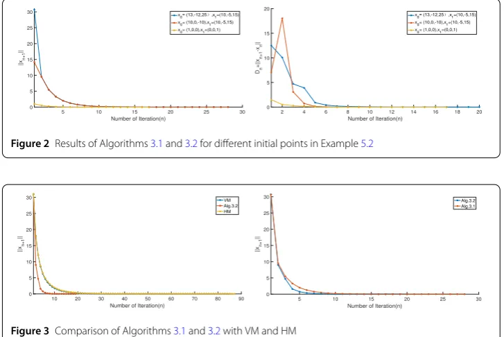
parametersβn=n_n–1₊₁,γn=_n+11 of Algorithm3.2. The experimental results of Algorithms3.1 and3.2are reported in Figs.2–3and Table1and Table2.

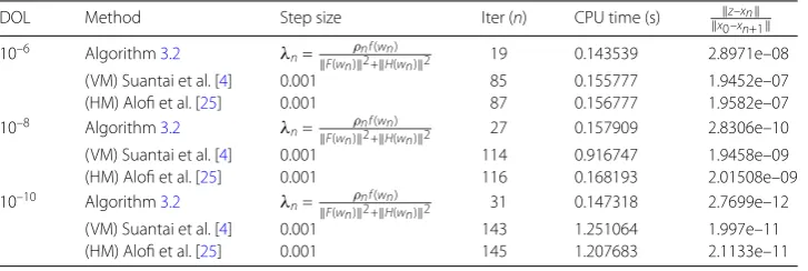
Figure 2Results of Algorithms3.1and3.2for different initial points in Example5.2

Figure 3Comparison of Algorithms3.1and3.2with VM and HM

Table 1 Convergence of the sequence in Algorithm3.1

n xn xn+1 wn xn+1–xn xn+1–wn

0 (13, –12, 25) (10, –5, 15) (9.998, –4.995, 14.993) 12.5750 0.0088 1 (10, –5, 15) (2.280, –7.305, 5.707) (2.277, –7.305, 5.703) 4.8141 0.0051 2 (2.280, –7.305, 5.707) (2.972, –3.161, 3.356) (2.973, –3.154, 3.352) 2.8272 0.0083 3 (2.972, –3.161, 3.356) (1.053, –2.830, 1.306) (1.047, –2.829, 1.299) 1.6818 0.0098 4 (1.053, –2.830, 1.306) (1.336, –1.229, 0.874) (1.338, –1.218, 0.871) 1.0192 0.0121 5 (1.336, –1.229, 0.874) (0.511, –1.101, 0.289) (0.498, –1.099, 0.281) 0.6520 0.0153 . . .

10 (0.106, –0.166, 0.006) (0.111, –0.063, 0.019) (0.111, –0.057, 0.020) 0.0700 0.0059 20 (0.334, –0.989, –0.329)e–04 (0.007, 0.269, 0.041)e–04 (–0.091, 0.647, 0.152)e–04 3.5041e–05 4.0568e–05 26 (–0.378, 0.219, –0.010)e–05 (–0.111, 0.156, 0.023)e–05 (–0.031, 0.136, 0.033)e–05 1.2179e–06 8.2810e–07 27 (–0.111, 0.156, 0.023)e–06 (–0.741, 0.424, –0.028)e–06 (–0.629, 0.085, –0.106)e–06 4.864e–07 1.44e–07

Table 2 Convergence of the sequence in Algorithm3.2

n xn xn+1 wn xn+1–xn xn+1–wn

0 (10, 0, –10) (–10, 5, 10) (–10.003, 5.001, 10.003) 28.7228 0.0039 1 (–10, 5, 10) (–2.985, 1.319, 4.384) (–2.981, 1.317, 4.379) 9.7107 0.0064 2 (–2.985, 1.319, 4.384) (–2.291, –0.037, 1.814) (–2.288, –0.043, 1.802) 2.9877 0.0134 3 (–2.291, –0.037, 1.814) (–1.033, 0.336, 1.048) (–1.018, 0.341, 1.039) 1.5187 0.0183 4 (–1.033, 0.336, 1.048) (–0.313, 0.343, 0.568) (–0.296, 0.344, 0.557) 0.8660 0.0204 5 (–0.313, 0.343, 0.568) (–0.332, 0.091, 0.225) (–0.332, 0.082, 0.212) 0.4264 0.0156 . . .

10 (–0.034, 0.009, 0.009) (–0.012, 0.011, 0.006) (–0.006, 0.012, 0.005) 0.0223 0.0059 20 (0.318, –0.203, 0.045)e–05 (0.311, –0.452, –0.013)e–06 (0.321, –0.128, 0.062)e–05 2.5567e–06 7.6702e–07 21 (0.311, –0.452, –0.013)e–06 (0.119, –0.167, –0.005)e–06 (0.059, –0.156, –0.020)e–05 2.0896e–06 6.2688e–07 22 (0.119, –0.167, –0.005)e–06 (0.879, –0.575, 0.075)e–06 (0.787, –0.246, 0.113)e–06 8.665e–07 3.432e–07

Figure 4Numerical results forK= 20

Table 3 Comparison of Algorithm3.2with other algorithms

DOL Method Step size Iter (n) CPU time (s) _xz–xn

0–xn+1

10–6 _{Algorithm3.2 λ}

n=_F( ρnf(wn)

wn)2+H(wn)2 19 0.143539 2.8971e–08

(VM) Suantai et al. [4] 0.001 85 0.155777 1.9452e–07 (HM) Alofi et al. [25] 0.001 87 0.156777 1.9582e–07 10–8 _{Algorithm3.2 λ}

n=_F( ρnf(wn)

wn)2+H(wn)2 27 0.157909 2.8306e–10

(VM) Suantai et al. [4] 0.001 114 0.916747 1.9458e–09 (HM) Alofi et al. [25] 0.001 116 0.168193 2.01508e–09 10–10 _{Algorithm3.2 λ}

n=_F( ρnf(wn)

wn)2+H(wn)2 31 0.147318 2.7699e–12

(VM) Suantai et al. [4] 0.001 143 1.251064 1.997e–11 (HM) Alofi et al. [25] 0.001 145 1.207683 2.1133e–11

5.2 Comparison of Algorithm3.2with other algorithms

In this part, we present several experiments to compare Algorithm3.2with other algo-rithms. Two algorithms used to compare are the viscosity method (VM) of Suantai et al. [4], and the Halpern-type method (HM) of Alofi et al. [25], in which the step size depends on the norm of operatorT. For the three algorithms, the operatorsA,B,T are defined as in Example5.2. In view of the fact that the normT 14.87, we take the step size λn= 0.001 in the algorithms of Suantai et al. [4] and Alofi et al. [25].

We set the parametersβn=2₂n_n–1₊₁,ρn= 3 –_n1₊₁ andγn=_2n1₊₁ in our Algorithm3.2;αn=

1

2n+1,βn=γn=

n

2n+1 and the contractionf(x) =

x

5 in Suantai et al. [4];βn=

n

2n+1,αn= 1 2n+1

andun= 0 in Alofi et al. [25]. In addition, we choose the stopping criterion for all the algorithmsxn+1–xn ≤DOL. Furthermore, we takex0= (13, –12, 25) and compare the

iterations and computer times. The experiment results are reported in Fig.4and Table3. From Table3, we can see that our Algorithm3.2is the best and seems to have a com-petitive advantage. However, as mentioned in the previous sections, the main advantage of our Algorithm3.2is that the inertial technique combined with self-adaptive step size is employed without the prior knowledge of operator norms.

5.3 Compressed sensing

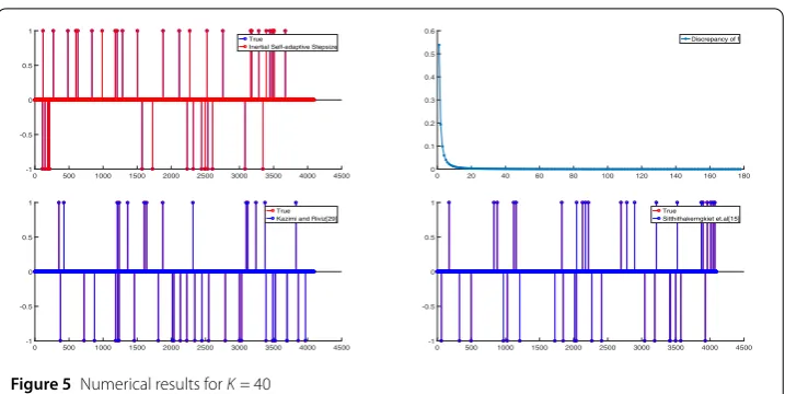
Table 4 Comparison of Algorithm3.2with those of Sitthithakerngkiet et al. [23] and Kazmi et al. [29]

K,mandn DOL Method Step size Iter (n)

K= 50,m= 210_{,n= 2}12 ₁₀–6 _{Algorithm3.2 λ}

n 1881 Sitthithakerngkiet et al. [23] 0.05 3262 Kazmi et al. [29] 0.05 28,674

K= 40,m= 210,n= 212 10–6 Algorithm3.2 λn 1779 Sitthithakerngkiet et al. [23] 0.05 2942 Kazmi et al. [29] 0.05 26,488

K= 20,m= 210_{,n= 2}12 ₁₀–6 _{Algorithm3.2 λ}

n 1496 Sitthithakerngkiet et al. [23] 0.05 2094 Kazmi et al. [29] 0.05 19,488

standard Gaussian distribution and vectorb=Ax+, where is additive noise. When = 0, there is no noise in the observed data. Our task is to recover signalx0from datab.

For further explanations, one can consult Nguyen and Shin [52].

For solving the problem, we recall the LASSO problem Tibshirani [53]:

min x∈Rn

1

2Ax–b

2 2,

s.t. x1≤t,

where t> 0 is a given constant. So, in relation with the SVIP (1.1)–(1.2), we consider

B–1

1 (0) ={x|x1≤t},B–12 (0) ={b}and define

B1(x) =

⎧ ⎨ ⎩

{u|sup_y1≤ty–x,u ≤0}, x∈C,

∅, else,

and define

B2(y) =

⎧ ⎨ ⎩

H2, y=b,

∅, else.

We set the parametersβn=2₂n_n–1₊₁,ρn= 3 –_n1₊₁ andγn=_2n1₊₁ in our Algorithm3.2and compare with the results of Sitthithakerngkiet et al. [23] and Kazmi et al. [29]. For the experiment setting we choose the following parameters:A∈Rm×nis generated randomly with m= 210, n= 212,x0∈Rn containsK-spikes with amplitude±1 distributed in the

whole domain randomly. In addition, for simplicity, we take f(x) = x₂,S=I, αi= _i+11 in [29] andSi=I,αi= 10–3/(i+ 1),βi= 0.5 – 1/(10i+ 2) in [23] andαi=_ii₊₁–1,γi=_i+11 in our algorithms. In addition, we taket=K in all the algorithms and the stopping criterion xn+1–xn ≤DOLwithDOL= 10–6. All the numerical results are presented in Table4 and Figs.4–5.

6 Conclusion

Figure 5Numerical results forK= 40

null point problem, many authors have dedicated their efforts to the construction of it-erative algorithms. However, the drawback of these algorithms is that either the step size depends on the linear bounded operator norm in Banach spaces or the maximal operator belongs to Hilbert spaces.

This motivated studying the solution set of the split common null point problem without prior knowledge of the operator norms in Banach spaces. The main result of this paper is a new inertial algorithm which incorporates the self-adaptive step size rule to solve the split null point problems for multi-valued maximal monotone operators in Banach spaces. To some extent, the weak and strong convergence theorems of the new inertial algorithm in this paper complement the approximating methods for the solution of split common null point problem and extend and unify some results (see, e.g., Byrne et al. [6], Takahashi [23], Alofi [25], Suantai et al. [4] and Promluang and Kuman [5]). In addition, the numerical examples and comparisons are presented to illustrate the efficiency and reliability of our algorithms.

Acknowledgements

The authors express their deep gratitude to the referee and the editor for his/her valuable comments and suggestions which helped tremendously in improving the quality of this paper and made it suitable for publication.

Funding

This article was funded by the National Science Foundation of China (11471059) and Science and Technology Research Project of Chongqing Municipal Education Commission (KJ 1706154) and the Research Project of Chongqing Technology and Business University (KFJJ2017069).

Competing interests

The authors declare that they have no competing interests. Authors’ contributions

All authors contributed equally to this work. All authors read and approved final manuscript.

Publisher’s Note

Springer Nature remains neutral with regard to jurisdictional claims in published maps and institutional affiliations. Received: 20 September 2018 Accepted: 15 January 2019

References

1. Alvarez, F., Attouch, H.: An inertial proximal method for maximal monotone operators via discretization of a nonlinear oscillator with damping. Set-Valued Anal.9, 3–11 (2001)

3. Takahashi, W.: The split common null point problem in Banach spaces. Arch. Math. (Basel)104(4), 357–365 (2015) 4. Suantai, S., Srisap, K., Naprang, N., Mamat, M., Yundon, V., Cholamjiak, J.: Convergence theorems for finding split

common null point problem in Banach spaces. Appl. Gen. Topol.18(2), 345–360 (2017)

5. Promluang, K., Kumam, P.: Viscosity approximation method for split common null point problems between Banach spaces and Hilbert spaces. J. Inform. Math. Sci.9(1), 27–44 (2017)

6. Byrne, C., Censor, Y., Gibali, A., Reich, S.: Weak and strong convergence of algorithms for the split common null point problem. J. Nonlinear Convex Anal.13, 759–775 (2012)

7. Censor, Y., Gibali, A., Reich, S.: Algorithms for the split variational inequality problem. Numer. Algorithms59, 301–323 (2012)

8. Censor, Y., Elfving, T.: A multi-projection algorithm using Bregman projections in product space. Numer. Algorithms8, 221–239 (1994)

9. Byrne, C.L.: Iterative projection onto conve sets using multiple Bregman distances. Inverse Probl.15, 1295–1313 (1999)

10. Rockafellar, R.T.: On maximal monotonicity of sums of nonlinear operators. Trans. Am. Math. Soc.149, 75–88 (1970) 11. Moudaf, A.: Split monotone variational inclusions. J. Optim. Theory Appl.150, 275–283 (2011)

12. Ansari, Q.H., Rehan, A., Wen, C.F.: Implicit and explicit algorithms for split common fixed point problems. J. Nonlinear Convex Anal.17(7), 1381–1397 (2016)

13. Ansari, Q.H., Rehan, A.: Split feasibility and fixed point problems. In: Ansari, Q.H. (ed.) Nonlinear Analysis: Approximation Theory, Optimization and Applications, pp. 281–322. Springer, New Delhi (2014)

14. Censor, Y., Bortfeld, T., Martin, B., Trofimov, A.: A unified approach for inversion problems in intensity modulated radiation therapy. Phys. Med. Biol.51, 2353–2365 (2003)

15. Ceng, L.C., Ansari, Q.H., Yao, J.C.: An extragradient method for solving split feasibility and fixed point problems. Comput. Math. Appl.64, 633–642 (2012)

16. Byrne, C.: Iterative oblique projection onto convex sets and the split feasibility problem. Inverse Probl.18, 441–453 (2002)

17. Byrne, C.: A unified treatment of some iterative algorithms in signal processing and image reconstruction. Inverse Probl.20, 103–120 (2004)

18. Yang, Q.: The relaxed CQ algorithm for solving the split feasibility problem. Inverse Probl.20, 1261–1266 (2004) 19. Moudafi, A., Thakur, B.S.: Solving proximal split feasibility problem without prior knowledge of matrix norms. Optim.

Lett.8(7), 2099–2110 (2013).https://doi.org/10.1007/s11590-013-0708-4

20. Gibali, A., Mai, D.T., Nguyen, T.V.: A new relaxed CQ algorithm for solving split feasibility problems in Hilbert spaces and its applications. J. Ind. Manag. Optim.2018, 1–25 (2018)

21. Shehu, Y., Iyiola, O.S.: Convergence analysis for the proximal split feasibility problem using an inertial extrapolation term method. J. Fixed Point Theory Appl.19, 2483–2510 (2017)

22. Ceng, L.C., Ansari, Q.H., Yao, J.C.: Mann type iterative methods for finding a common solution of split feasibility and fixed point problems. Positivity16(3), 471–495 (2012)

23. Sitthithakerngkiet, K., Deepho, J., Kumam, P.: Convergence analysis of a general iterative algorithm for finding a common solution o split variational inclusion and optimization problems. Numer. Algorithms (2018). https://doi.org/10.1007/s11075-017-0462-2

24. Takahashi, W., Yao, J.C.: Strong convergence theorems by hybrid methods for the split common null point problem in Banach spaces. Fixed Point Theory Appl.2015, Article ID 87 (2015)

25. Alofi, A.S., Alsulami, M., Takahashi, W.: Strongly convergent iterative method for the split common null point problem in Banach spaces. J. Nonlinear Convex Anal.2, 311–324 (2016)

26. Kamimura, S., Takahashi, W.: Strong convergence of proximal-type algorithm in Banach spaces. SIAM J. Optim.13, 938–945 (2002)

27. Takahashi, W.: The split common null point problem for generalized resolvents in two Banach spaces. Numer. Algorithms75(4), 1065–1078 (2017)

28. Ansari, Q.H., Rehan, A.: Iterative methods for generalized split feasibility problems in Banach spaces. Carpath. J. Math. 33(1), 9–26 (2017)

29. Kazmi, K.R., Rizvi, S.H.: An iterative method for split variational inclusion problem and fixed point problem for a nonexpansive mapping. Optim. Lett.8, 1113–1124 (2014)

30. Mainge, P.E.: Convergence theorem for inertial KM-type algorithms. J. Comput. Appl. Math.219, 223–236 (2008) 31. Alvarez, F.: On the minimizing property of a second order dissipative system in Hilbert spaces. SIAM J. Control Optim.

38(4), 1102–1119 (2000)

32. Alvarez, F.: Weak convergence of a relaxed and inertial hybrid projection-proximal point algorithm for maximal monotone operators in Hilbert space. SIAM J. Optim.14(3), 773–782 (2003)

33. Chang, S.S., Cho Zhou, Y.J., Zhou, H.Z.: Iterative Methods for Nonlinear Operator Equation in Banach Spaces. Nova Science Publishers, Huntington (2002)

34. Chidume, C.: Geometric Properties of Banach Spaces and Nonlinear Iterations. Lecture Note in Mathematics, vol. 1965. Springer, London (2009)

35. Browder, F.E.: Nonlinear maximal monotone operators in Banach spaces. Math. Ann.175, 89–113 (1968) 36. Takashi, W.: Convex Analysis and Approximation of Fixed Point. Yokohama Publishers, Yokohama (2009) 37. Kohsaka, F., Takahashi, W.: Existence and approximation of fixed points of firmly nonexpansive-type mappings in

Banach spaces. SIAM J. Optim.19(2), 824–835 (2008)

38. Kohsaka, F., Takahashi, W.: Fixed point theorems for a class of nonlinear mappings related to maximal monotone operators in Banach spaces. Arch. Math.91(2), 166–177 (2008)

39. Aoyama, K., Kohsaka, F., Takahashi, W.: Three generalizations of firmly nonexpansive mappings: their relations and continuity properties. J. Nonlinear Convex Anal.10(1), 131–147 (2009)

40. Bauschke, H.H., Wang, X.F., Yao, L.J.: General resolvents for monotone operators: characterization and extension (2008).arXiv:0810.3905v1

41. Xu, H.K.: Iterative algorithms for nonlinear operators. J. Lond. Math. Soc.66(2), 240–256 (2002)