ABSTRACT
Park, Man Sik. Symmetry and Separability In Spatial-Temporal Processes.
(Un-der the direction of Dr. Montserrat Fuentes.)
Symmetry is one of most standard assumptions that are needed for a
covari-ance function in spatial statistics. However, many studies in spatial research fields
show that environmental data have complex spatial-temporal dependency
struc-tures that are difficult to model and estimate, due to the lack of symmetry and
other standard assumptions of a covariance function. So, not much literature
exists in statistics about asymmetric covariance functions and formal tests for
lack of symmetry in spatial-temporal processes. In this study, we introduce
cer-tain types of symmetry in spatial-temporal processes and propose new classes of
asymmetric spatial-temporal covariance models by using spectral representations.
We also clarify the relationship between symmetry and separability and introduce
nonseparable covariance models. Based on the proposed concept of symmetry in
spatial-temporal processes, new formal tests for lack of symmetry are proposed
in this study by employing spectral representations of the spatial-temporal
co-variance function. The advantage of the tests is that simple analysis of co-variance
(ANOVA) approaches are employed for detecting lack of symmetry inherent in
spatial-temporal processes. Our new classes of covariance models are applied to
the methods for the fine particulate matters with a mass median diameter less than
Symmetry and Separability In Spatial-Temporal Processes
by
Man Sik Park
A dissertation submitted to the Graduate Faculty of North Carolina State University
in partial fulfillment of the requirements for the Degree of
Doctor of Philosophy
STATISTICS
Raleigh
2005
APPROVED BY:
Dr. Montserrat Fuentes Dr. Peter Bloomfield
Chair of Advisory Committee
Dr. David A. Dickey Dr. Sastry G. Pantula
Biography
Man Sik Park was born in Youngdong, Republic of Korea on October 1, 1972. He
entered the Department of Statistics at Korea University in 1991 and earned his
B.S. in 1998 and M.S. in 2000 in mathematical statistics. He joined the department
of Statistics, North Carolina State University for the pursuit of Ph.D. degree.
He has been accepted as a post-doctoral research position in the department of
Acknowledgements
I would like to thank the members of my advisory committee for their advice and
support during the preparation of my dissertation.
I am extremely grateful for having Dr.Montserrat Fuentes as my advisor. Her
enthusiasm, knowledgeable guidance, and constant support, including financial
support, have meant a tremendous amount to me. She is not only an excellent
researcher who imposes the highest standards on her academic work, but also an
outstanding advisor who provides continuing encouragement for her students. I
thank her for her encouragement to become an independent researcher, and I also
admire tireless energy and her devotion to her professional career.
Thanks to Dr. Peter Bloomfield for his valuable comments and suggestions
on spectral analysis approaches. Thanks to Dr. Dave A. Dickey for his advice
and encouragement during my work on my dissertation. Thanks to Dr.
Sas-try G. Pantula for his helpful questions and suggestions that have helped me to
present the material much better. I also would like to thank Dr. William H.
Swallow and all my professors, Terry Byron, and Adrian Blue for all their help
and encouragement over these past 3 years. I am also grateful to Dr. David M.
Holland, my collaborator, working at EPA for his insightful comments about the
real applications.
Finally I would like to express my deepest gratitude and biggest appreciation
to my parents. I also would like to thank my wife, Eunnam, and my son, Robin,
Contents
List of Tables vii
List of Figures viii
1 Introduction 1
2 New Classes of Asymmetric Spatial-Temporal Covariance
Mod-els 6
2.1 Introduction . . . 6
2.2 Symmetry in Spatial-Temporal Processes . . . 10
2.3 Classes of Asymmetric Stationary Covariance Models . . . 12
2.4 Symmetry and Separability . . . 22
2.5 Real Application . . . 26
2.6 Discussion . . . 32
3 Testing Lack of Symmetry in Spatial-Temporal Processes 37 3.1 Introduction . . . 37
3.2 Spectral Representation of Stationary Spatial-Temporal Processes 41 3.3 Tests for Lack of Symmetry In Spatial-Temporal Processes . . . . 42
3.3.1 Test for Lack of Axial Symmetry in Time . . . 44
3.3.2 Test for Lack of Axial Symmetry in Space . . . 51
3.4 Simulation Study . . . 57
3.4.1 Testing Lack of Axial Symmetry in Time . . . 60
3.4.2 Testing Lack of Axial Symmetry in Space . . . 62
3.5 Real Application . . . 66
3.5.1 Testing Lack of Axial Symmetry in Time . . . 68
3.5.2 Testing Lack of Axial Symmetry in Space . . . 71
3.6 Discussion . . . 75
5 Appendix 79
5.1 The derivation of the asymmetric stationary spatial-temporal co-variance function . . . 79 5.2 The asymptotic normality of φ∗ab(τ) in (3.18) . . . 80
List of Tables
2.1 Square-root of mean squared prediction errors based on the WLS
and the ML estimation methods at the two reserved stations. . . . 31
2.2 Parameter Estimates based on Gaussian Asymmetric Spatial-Temporal Covariance from WLS and ML methods. Note that (−4)≡10−4. . 34
3.1 Empirical Powers of an Alternative Hypothesis that v1 = 0 but v2 = 0. Note that the situation that v1 = 0 but v2 = 0 is the vertical dotted line in each plot of Figure 3.2. . . 62
3.2 Empirical Powers of an Alternative Hypothesis meaning the dashed lines in the plots of Figure 3.5. . . 66
3.3 Analysis of variance . . . 69
3.4 Analysis of variance . . . 73
3.5 Analysis of variance . . . 76
List of Figures
1.1 Isotropy in Two-Dimensional Space . . . 3 1.2 Geometric Anisotropy in Two-Dimensional Space . . . 4
2.1 Contour plots forC(h;u) axially symmetric in time (v=0), where each number in plot indicates the corresponding percentile of the covariance withγ = 1, andν=d= 2. (a) Contour plot ofCversus h1 and h2 for all u, where α= 0.02 and β = 1; (b) contour plot of C versus h1 (or h2) and u, where α =√2 and β = 1; (c) contour plot ofC withα = 0.02,0.03,0.04 andβ = 1. Dotted line is for the first case, solid line for the second, and dashed line for the third. . 15 2.2 Contour plots forC(h;u) axially symmetric in space (v1 = 0.01, v2 =
0), where γ = 1, ν = d = 2, α = 0.02 and β = 1. (a) Contour plot of C versus h1 and h2 for u = −10,0,10; (b) contour plot of C versus h1 and u for all h2; (c) contour plot ofC versush2 and u for h1 =−200,0,200. . . 17 2.3 Contour plots forC(h;u) digonally symmetric in space (v1 =v2 =
v0 = 0.01), where γ = 1, ν = d = 2, α = 0.02 and β = 1. (a) Contour plot of C versus h1 and h2 for u=−10,0,10; (b) contour plot ofC versush1 (h2) anduforh2 (h1)=−200,0,200; (c) contour plot of C versus h1 and h2 for v0 = 0,0.005,0.01 and u = 10; (d) contour plot ofCversush1 andh2 forv0 = 0,0.005,0.01 andu=−10. 18 2.4 Contour plots for C(h;u) asymmetric in space and time versus h1
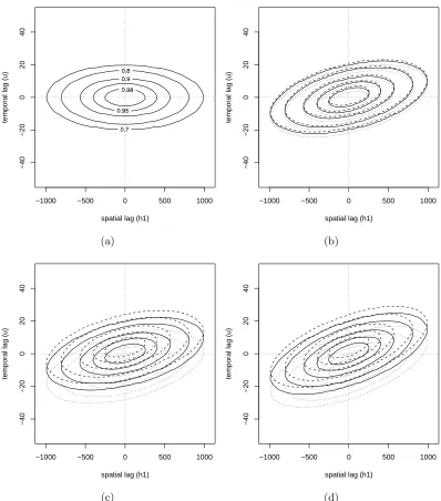
and h2 for u = −10,0,10, where γ = 1, ν =d = 2, α = 0.02, and β = 1. (a) v = (0,0); (b) v = (0.01,0.005); (c) v = (0.01,0.02); (d) v= (0.015,0.02). . . 19 2.5 Contour plots for C(h;u) asymmetric in space and time versus h1
2.6 Contour plots for C(h;u) asymmetric in space and time versus h2 andufor h1 =−400,0,400, where γ = 1,ν =d= 2, α= 0.02, and β = 1. (a) v = (0,0); (b) v = (0.01,0.005); (c) v = (0.01,0.02); (d) v= (0.015,0.02). . . 21 2.7 Relationship between symmetry and separability . . . 24 2.8 The map of the 18 monitoring stations in the northeastern U.S. . 27 2.9 Kriging maps based on the ML estimates in Table 2.2 for each
model. Note that the interpolation is performed at the regular grids on August 31, 2003. . . 30 2.10 Scatter plots of the observed values at the first reserved station
and the ML predicted values obtained from each covariance model. Note that the dashed line stands for the perfect relationship. . . . 35 2.11 Scatter plots of the observed values at the second reserved station
and the ML predicted values obtained from each covariance model. Note that the dashed line stands for the perfect relationship. . . . 36
3.1 Selection of Pairs for the Test for Lack of Axial symmetry in Time. Note that we consider four different directions in spatial domain; ENE (D1), NNE (D2), NNW (D3), and WNW (D4). . . 60 3.2 The Contour Plots of Empirical Powers Under General Asymmetry
in Space and Time for Main Effects from ANOVA Technique. Note that the dotted lines are about axial symmetry in space and the dashed line is for diagonal symmetry in space, and the null hypoth-esis is located on the origin (v= 0). (a) Empirical powers for the effect of “Direction”; (b) empirical powers for the effect of “Tem-poral Frequency”; (c) empirical powers for the effect of “Subregion”. 61 3.3 Selection of Pairs for the Test for Lack of Axial symmetry in Space.
Note that we consider the two different directions in two dimen-sional (spatial-temporal) domain; D5 and D6. . . 63 3.4 The Contour Plots of Empirical Powers Under General Asymmetry
in Space and Time for Main Effects from ANOVA Technique. Note that the vertical dotted line is the null hypothesis, axial symmetry in space (v1 = 0,v2 = 0). (a) Empirical powers for the effect of “Di-rection”; (b) empirical powers for the effect of “Spatial Frequency”; (c) empirical powers for the effect of “Subregion”. . . 64 3.5 The Contour Plots of Empirical Powers Under General Asymmetry
3.6 The map of the locations of 3721 (= 61×61) centroids of grid cells where each cell is size of 36km×36km. Note that the numbers on the right of grid cells are row indice and the ones on the top are column indice. . . 67 3.7 The plot of the locations of the selected 16 pairs. Note that four
different directions are considered; ENE direction (D1), NNE di-rection (D2), NNW didi-rection (D3), and WNW (D4). . . 68 3.8 The QQplots of the residuals (a) The quantiles fromN(0,1) versus
the residuals in case of ENE direction (D1); (b) the quantiles from N(0,1) versus the residuals in case of WNW direction (D4). . . . 71 3.9 The plot of the locations of the selected 16 pairs. Note that two
directions are considered; D5, D6. . . 72 3.10 The QQplot of the residuals from the ANOVA technique in case of
Chapter 1
Introduction
The most common problem that researchers in diverse fields such as
epidemiol-ogy, ecolepidemiol-ogy, climatolepidemiol-ogy, and environmental health research are confronted with
is how to predict the observations at unobserved sites using the given data. To
do that, they estimate the underlying parameters in certain covariance structures
that are assumed to explain the given data very well. Most data are observed in
space and time. Both spatial and temporal effects are considered for the spatial
interpolation and the temporal forecast.
In general, the spatial-temporal processes have a much more complicated
struc-ture than spatial process alone. Since spatial strucstruc-ture and temporal strucstruc-ture are
entangled in the covariance structure, it is not easy to model these two parts
simul-taneously. In order to overcome the difficulty in modelling the spatial-temporal
covariance structure, the concept of “separability” has been applied. A
divided into a spatial covariance and temporal covariance, separately. Separable
spatial-temporal classes give us many advantages, such as the simplified
repre-sentation of the covariance matrix and, consequently, important computational
benefits. But in real applications, it may not be reasonable to estimate the
co-variances that depend on space and time separately and combine them together
for predicting observations at unobserved sites or times. Many reseachers (Cressie
and Huang (1999), Gneiting (2002) and so on) have proposed nonseparable
co-variance classes for spatial-temporal processes. Recently Fuentes et al. (2005)
introduced a new nonseparable class with a unique parameter reflecting the
de-pendency between the spatial and temporal components.
“Isotropy” is also one of the common problems that the researchers should
take into account when analyzing data. A spatial process is isotropic if the
co-variance between any two arbitrary sites only depends on the distance no matter
what the relative position between them is. As you can see from Figure 1.1,
un-der the isotropic condition, the covariance between a and b is the same as the
covariance between a and b because of the same distance, r1. So, the isotropic covariance in two-dimensional space does not depend on any direction. This
con-dition, however, is too unrealistic to apply to real conditions. We can enumerate
many examples that do not satisfy the isotropic condition. The dispersion of air
pollutants from a chemical factory is directly affected by the wind speed as well
as wind direction. The patterns of annual temperature in United States can be
r1
r1
a
b b'
r2
r2
c' c
X Y
Figure 1.1: Isotropy in Two-Dimensional Space
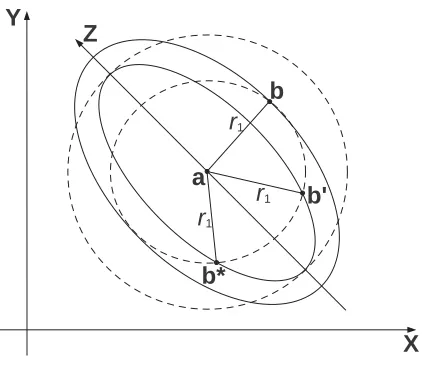
So “anisotropy” should be considered. Anisotropic covariance depends not only
on distance between sites but also on their relative orientation. As one can see
from Figure 1.2, the covariance between a and b is different from the covariance
between a and b despite separation by the same distance, r1. In order to check the existence of certain types of anisotropy, we make use of a “rose diagram” or
a “directional semivariogram”. Then, we transform the covariance structure to
achieve isotropy. Geometric anisotropy is the simplest case. We can make the
covariance structure satisfy isotropy by estimating the parameters for strength
and rotation. Zimmerman (1993) proposes three different kinds of nongeometric
anisotropy: 1) sill anisotropy; 2) nugget anisotropy; and 3) range anisotropy.
Fig-ure 2 shows another important infomation that has not been considered so far.
r1
r1
a
b b'
X Y
r1
b* Z
Figure 1.2: Geometric Anisotropy in Two-Dimensional Space
betweenaandb∗ and betweenaand b are symmetric with respect toZ-axis. So anisotropy may present some patterns of spatial or spatial-temporal dependency,
which can be specified by “symmetry”. A few researchers have dealt with
sym-metry in the environmental field. Scaccia and Martin (2005) introduced certain
types of symmetry in the spatial processes: 1) axial symmetry; 2) diagonal
sym-metry; and 3) complete symmetry, and proposed some tests for symmetry using
spectral methods. Their work, however, focuses on only two dimensional spatial
process ignoring time effect, and is applied to a complete regular lattice
struc-ture. In spatial-temporal processes there can be four different types of symmetry
in spatial-temporal processes: 1) axial symmetry in time; 2) axial symmetry in
space; 3) diagonal symmetry in time; and 4) diagonal symmetry in space.
provide some advantages to help researchers construct simplified covariance
struc-tures for spatial-temporal processes, and to make better interpretations of the
un-derlying characteristics of the processes. The differences between separability and
symmetry, however, are apparent. Separability only takes into account temporal
lag and spatial separation, which consists of the product of two covariance
func-tions. Symmetry, however, takes into account each spatial lag as well as temporal
lag. So, in spatial-temporal processes, separability does not always guarantee
sym-metry. Since it is difficult to statistically determine isotropy in spatial-temporal
processes, symmetry can play an important role as its substitute.
In this study, we characterize the aforementioned types of symmetry in
spatial-temporal processes, and develop a new testing method for each case of symmetry
with asymptotic properties of cross-spectral density function and coherency.
Fi-nally, we develop a new class of nonsymmetric spatial-temporal stationary
covari-ance models.
This study is organized as follows. In chapter 2, we introduce new concepts
of symmetry inherent to spatial-temporal processes, develop a new class of
asym-metric spatial-temporal stationary covariance models, and apply our new class to
the real application. In chapter 3, we propose new formal tests for lack of
sym-metry by employing the spectral representations of spatial-temporal covariance
function and validate the tests with the simulation study and the the application
to air-pollution datasets. Chapter 4 focuses on the conclusion and the further
Chapter 2
New Classes of Asymmetric
Spatial-Temporal Covariance
Models
2.1
Introduction
Many studies in diverse fields such as climatology, ecology, and public health
research show that environmental data have complex spatial-temporal
depen-dency structures that are difficult to model and estimate. In general, the
spatial-temporal processes have more complicated structures than the spatial processes
alone. The main reason is that, since the spatial and the temporal structure are
entangled in the covariance function, it is not easy to take into account these
two structures simultaneously. In order to overcome the difficulty in building
spatial-temporal processes: separability and symmetry.
Separability in spatial-temporal processes enables us to easily construct the
model due to advantages such as the simplified representation of the covariance
matrix, consequently, remarkable computational benefit. Suppose that {Z(s, t) :
s ∈ D ⊂ Rd, t ∈ [0,∞)} denote a stationary spatial-temporal process measured atN sites and T times, and the covariance function is defined as
C(si−sj;tk−tl|θ)≡cov{Z(si, tk), Z(sj, tl)}; si,sj ∈D, tk, tl∈[0,∞),(2.1)
where si = (si
1,· · · , sid) and C satisfies the positive definiteness for all θ ∈Θ ⊂ Rp. Then the process is called separable if the covariance function in (2.1) can be divided into a spatial covariance and temporal covariance, that is,
C(si−sj;tk−tl|θ) =Cs(si−sj|θs)·CT(tk−tl|θt), (2.2)
where Cs is a positive definite spatial covariance function in Rd, C
T is a positive definite temporal covariance function inR1, and θ= (θs,θt). Under stationarity condition, (2.2) is rewritten as
C(h;u|θ) =Cs(h|θs)·CT(u|θt), (2.3)
for allh ≡(h1,· · ·, hd) =si−sj is a vector of spatial lags and allu=tk−tl is a temporal lag (see Rodriguez-Iturbe and Majia (1974)). However, in real
applica-tions, it may not be reasonable to estimate the covariance functions that depend
on space and time separately, and then, combine them together for predicting
not easy to capture the underlying pattern just by relying on separability. Many
reseachers have proposed nonseparable covariance classes for spatial-temporal
pro-cesses. Jones and Zhang (1997) develop a parametric family of spectral density
functions, with corresponding nonseparable stationary covariance functions, by
adapting stochastic partial differential equations. Cressie and Huang (1999)
in-troduce new classes of nonseparable, spatial-temporal stationary covariance
func-tions with space-time interaction. The separable covariance function is a special
case. Their main idea is to develop the nonseparable positive-definite covariance
function with spatial-temporal interaction by specifying two appropriate functions
each of which is expressed as a spectral representation in closed form. Gneiting
(2002) proposes general classes of nonseparable, stationary spatial-temporal
co-variance functions which are directly constructed in the space-time domain and
are based on Fourier-free implementation. This paper insists that any
spatial-temporal covariance function can be modeled without the Fourier transformation
as long as one finds appropriate functions. Recently Fuentes et al. (2005)
in-troduce a new class of nonseparable covariance models with a unique parameter
reflecting the dependency between the spatial and the temporal components.
In-stead of a covariance function which is the multiplication of spatial and temporal
covariances (see (2.3)), Myers and Journel (1990), and Rouhani and Myers (1990)
consider the separability under which the covariance function is the addition of
spatial and temporal covariances (see (2.2)), although the covariance matrix turns
The other concept for relieving the difficulty in modeling is symmetry.
Sym-metry also has the same advantages as separability does. SymSym-metry plays an
important role in helping researchers construct simplified covariance structures
for spatial-temporal processes, and making better interpretations of the
under-lying characteristics of the processes. Due to these benefits symmetry has been
assumed and even, has been taken for granted. In these days, more attention
has been focused on lack of symmetry although only a few studies have been
ac-complished so far. One of the noteworthy studies is Scaccia and Martin (2005),
which, for a spatial process, {Z(s) : s∈D⊂Rd}, especially for two-dimensional spatial lattice data, introduce two types of symmetry (axial symmetry; diagonal
symmetry) and separability which are, respectively, denoted by, for all h1 and h2
C(h1, h2) =C(−h1, h2), (2.4)
C(h1, h2) = C(h2, h1), (2.5)
and
C(h1, h2) = C1(h1)·C2(h2), (2.6)
where C(h1, h2) ≡ cov(Z(s1 + h1, s2 + h2), Z(s1, s2)), and C1 and C2 are the
positive-definite covariances of first and second spatial lag. They also develop
new tests for axial symmetry in (2.4) and separability in (2.6) based on
pe-riodograms. Using certain ratios of spatial periodograms, Lu and Zimmerman
(2005) propose new diagnostic tests for axial symmetry and complete symmetry
trial for adapting symmetry to the general spatial-temporal setting except Stein
(2005), which proposes spatial-temporal covariance models with lack of axial
sym-metry in time presented in Section 2.2. The approach in this study is based on
generating asymmetric models from symmetric ones by taking derivatives. In
this study we introduce certain types of symmetry in spatial-temporal processes,
and propose new classes of nonseparable spatial-temporal covariance models with
spatial-temporal dependency parameters. These classes are directly derived from
a simple and valid spectral density function and, hence, are represented in closed
form.
This chapter is organized as follows. In Section 2.2, we define three types
of symmetry realized in the spatial-temporal setting. Based on the definition of
symmetry we develop new classes of nonseparable covariance models in Section 2.3.
In Section 2.4, we clarify the relationship between symmetry and separability and
extend the proposed models to the nonseparable case. In Section 2.5, the proposed
covariance models will be fitted to spatial-temporal data on Particulate Matter
with a mass median diameter less than 2.5 µm (PM2.5) over the northeastern region of U.S. Finally, we briefly discuss our approach in Section 2.6.
2.2
Symmetry in Spatial-Temporal Processes
In this section, we define three types of symmetry in spatial-temporal
in space. In this article we assume that any covariance function is stationary in
time unless otherwise mentioned. The first type of symmetry is axial symmetry
in time.
Definition 2.2.1 A process is called axially symmetric in time if for any temporal
lag u= 0,
C(si−sj;u) =C(si∗ −sj∗;−u), (2.7)
for arbitrary four locations (i, j, i∗, j∗) satisfying si−sj =si∗−sj∗.
Under stationarity in space, (2.7) is reduced to
C(h;u) = C(h;−u), (2.8)
wheresi =sj+h andsi∗ =sj∗+h. What is important here is that the directions
and the distances on spatial domain are the same, and the temporal lags have
the same magnitudes but different signs. The second type of symmetry is axial
symmetry in space.
Definition 2.2.2 A process is called axially symmetric in space if
C(h;u) = C(˚h;u), (2.9)
where ˚h= (h1,· · · , hk−1,−hk, hk+1,· · · , hd) for k fixed.
As can be seen in (2.9), for temporal lagu fixed, all the spatial lags are the same
except one spatial lag, which has different sign. The process can be also called
Definition 2.2.3 A process is called (k-l) diagonally symmetric in space if
C(h;u) = C(¨h;u), (2.10)
where h¨ = (h1,· · · , hk−1, hl, hk+1,· · · , hl−1, hk, hl+1,· · · , hd) for k =l.
From (2.10) we can see that only two spatial lags, hk and hl, are switched with each other. Provided that d= 2, ¨h= (h2, h1).
2.3
Classes of Asymmetric Stationary
Covari-ance Models
We defined three different types of symmetry in spatial-temporal processes
in Section 2.2. Now we propose new classes of asymmetric spatial-temporal
sta-tionary covariance models. In this section, we provide a new and simple method
to construct such covariance models. The main idea of our approach is to build
covariance functions directly derived from the corresponding spectral density
tions. In order to do that, we propose the spatial-temporal spectral density
func-tion given by
fv(ω;τ) =γα2β2+β2ω+τv12+α2(τ +v2ω)2−ν =f0(ω+τv1;τ +v2ω),
(2.11)
where f0(ω;τ) ≡ γ(α2β2 +β2ω2 +α2τ2)−ν is the spectral density function transformed from an simple stationary spatial-temporal covariance function,γ, α
andβ are positive,ν > d+12 , and|v1v2|<1. Herev1 ={v1i}d
in (2.11) is always valid and its Fourier transformation always exists because the
following two conditions are satisfied:
C.1 fv(ω;τ)>0 everywhere
C.2 fv(ω;τ)<∞for all v1, v2 ∈Rd satisfying |v1v2|<1.
So, Cv(h;u) =RdRexp{ihω+iuτ}fv(ω;τ)dτ dω exists and has the positive-definiteness. We can write the corresponding covariance function from the spectral
density function, fv in (2.11) as
Cv(h;u) =
Rd
R
exp{ihω+iuτ}f0(ω+τv1;τ +v2ω)dτ dω
= Rd R exp
i(h−uv2) 1−v1v2 ω+i
(u−hv1) 1−v1v2 τ
f0(ω;τ)
1−v1v2 dτ dω
= 1
1−v1v2 C0
h−uv2
1−v1v2;
u−hv1
1−v1v2
,
(2.12)
where C0 is a simple stationary spatial-temporal covariance function, and
h=
hi
d
i=1 = 1−
j=i v1jv2j
hi+v2i j=i
v1jhj
d
i=1 .
By straightforward derivation with help of Stein (2005), and Gradshteyn and
Ryzhik (2000) (see Appendix), we finally obtain the closed form of the (d+ 1)
dimensional Mat´ern-type covariance function denoted by
Cv(h;u) = 1 1−v1v2 ×
γπ(d+1)/2α−2ν+dβ−2ν+1 2ν−(d+1)/2−1Γ(ν)
× Mν−d+1 2 ⎛ ⎜ ⎝
αh−uv2
1−v1v2 2
+
β(u−hv1) 1−v1v2
2 ⎞
⎟ ⎠,
where Mν(r) = rνK
ν(r) and · denotes the Euclidean distance. Here Kν is a modified Bessel function of the third kind of order ν. Before going further,
we explain the characteristics of the covariance parameters. α and β explain the
decaying rates of the spatial and the temporal correlations. So their inverses are
interpreted as spatial and temporal ranges. ν measures the degree of smoothness,
which means that the larger the ν is, the smoother a process is. What is more
important here are the asymmetry vectors v1 and v2. As one can see in (2.12)
and (2.13), u−hv1 is a temporal lag adjusted by a vector of spatial lags and
h−uv2 is a vector of spatial lags adjusted by a temporal lag. So, we can see
that the units ofv1 are temporal lag divided by spatial lags, which are called the
inverse of speeds. We can also know that the units of v2 are spatial lags over
temporal lag, which are called the velocities. In the rest of this section, we regard
the space-time domain as three-dimensional space for the better understanding.
v1 and v2 take part in developing new classes of asymmetric covariance models
and yield the covariance models with the following types of symmetry:
T.1 axial symmetry in time if v1 =v2 =0
T.2 axial symmetry in space if v11 = 0 or v21= 0 and v12 =v22= 0
T.3 diagonal symmetry in space if v11 =v12= 0 and v21=v22= 0
T.4 asymmetry in space and time otherwise.
spatial lag (h1)
spatial lag (h2)
−1000 −500 0 500 1000
−1000 −500 0 500 1000 (a)
spatial lag (h1 or h2)
temporal lag (u)
−1000 −500 0 500 1000
−40 −20 0 2 0 4 0 (b)
spatial lag (h1 or h2)
temporal lag (u)
−1000 −500 0 500 1000
−40 −20 0 2 0 4 0 (c)
Figure 2.1: Contour plots for C(h;u) axially symmetric in time (v = 0), where each number in plot indicates the corresponding percentile of the covariance with γ = 1, and ν = d = 2. (a) Contour plot of C versus h1 and h2 for all u, where α= 0.02 andβ = 1; (b) contour plot ofC versush1 (or h2) andu, whereα =√2 and β = 1; (c) contour plot of C withα = 0.02,0.03,0.04 and β= 1. Dotted line is for the first case, solid line for the second, and dashed line for the third.
point of view ofv= (v1, v2) inT.1–T.4. For the simplification of an asymmetric covariance function in (2.13), we can consider, as special cases, the two covariance
models as follow:
Cv1(h;u) =γπ
(d+1)/2α−2ν+dβ−2ν+1 2ν−(d+1)/2−1Γ(ν)
⎛ ⎝α
β(u−hv1) α
2
+h2 ⎞ ⎠
ν−d+1 2
× Kν−d+1 2
⎛ ⎝α
β(u−hv1) α
2
+h2 ⎞ ⎠,
(2.14)
and
Cv2(h;u) =γπ
(d+1)/2α−2ν+dβ−2ν+1 2ν−(d+1)/2−1Γ(ν)
⎛ ⎝α βu α 2
+h−uv22 ⎞ ⎠
ν−d+1 2
× Kν−d+1 2 ⎛ ⎝α βu α 2
+h−uv22 ⎞ ⎠.
The corresponding spectral density functions are, respectively, given by
fv1(ω;τ) = γα2β2+β2ω+τv12+α2τ2−ν =f0(ω+τv1;τ),
(2.16)
and
fv2(ω;τ) = γα2β2+β2ω2+α2(τ+v2ω)2−ν =f0(ω;τ+v2ω).
(2.17)
It is certain that both fv1(ω;τ) and fv2(ω;τ) are valid, so the corresponding covariance functions in (2.14) and (2.15) are always positive-definite.
Now we talk about the characteristics of an asymmetric stationary covariance
function in (2.14) derived from (2.16). As you can see, v1 controls the types of
symmetry inhereent in spatial-temporal processes. Figure 2.1 displays the
behav-iors of a spatial-temporal covariance function axially symmetric in time. As one
can see, under the axial symmetry in time, the covariance function with the center
of the origin always stays whateverh andu are (Figure 2.1(a),(b)). The decaying
rate parameters,α andβ only change the shape (Figure 2.1(c)). Figure 2.2 shows
that the pattern of a covariance axially symmtric in space depends on temporal
lag,uas well as a spatial lag,h1 noth2. As one can see, a process with the
covari-ance function moves on the axes of longitudinal lag, h1 and temporal lag, u, and
the direction of movement depends on the signs of uand h1, respectively (Figure
2.2(a),(c)). From Figure 2.2(b), we know that the the term about temporal effect,
spatial lag (h1)
spatial lag (h2)
−1000 −500 0 500 1000
−1000 −500 0 500 1000 (a)
spatial lag (h1)
temporal lag (u)
−1000 −500 0 500 1000
−40 −20 0 2 0 4 0 (b)
spatial lag (h2)
temporal lag (u)
−1000 −500 0 500 1000
−40 −20 0 2 0 4 0 (c)
Figure 2.2: Contour plots forC(h;u) axially symmetric in space (v1 = 0.01, v2 = 0), where γ = 1, ν = d = 2, α = 0.02 and β = 1. (a) Contour plot of C versus h1 and h2 for u=−10,0,10; (b) contour plot of C versus h1 and u for all h2; (c) contour plot of C versus h2 and u forh1 =−200,0,200.
Unlike the covariance function axially symmetric in space, this covariance
func-tion moves along a 45 degree line in the spatial domain (Figure 2.3(a)) and along
with the axis ofu(Figure 2.3(b)). Figure 2.3(b) also says that the ratio ofα toβ
is strongly related to the obliqueness of the shape. The asymmetry vector v also
changes the shape and the centroid (Figure 2.3(c),(d)). Figure 2.4 through 2.6
display the patterns of a covariance function which is asymmetric in space and
time. From Figure 2.4, we see that the covariance function does not move along
with 45 degree line on spatial domain and the moving speed and the angle of line
connecting the centroids are influenced by each element of v (Figure 2.4(b)-(d)).
This figure also shows that the shape changes in comparison to that of a
covari-ance symmetric in time (Figure 2.4(a)). Figure 2.5 and 2.6 illustrate the contour
plots of a covariance function asymmetric in space and time versus each spatial
spatial lag (h1)
spatial lag (h2)
−1000 −500 0 500 1000
−1000
−500
0
500
1000
(a)
spatial lag (h1 or h2)
temporal lag (u)
−1000 −500 0 500 1000
−40
−20
0
2
0
4
0
(b)
spatial lag (h1)
spatial lag (h2)
−1000 −500 0 500 1000
−1000
−500
0
500
1000
(c)
spatial lag (h1)
spatial lag (h2)
−1000 −500 0 500 1000
−1000
−500
0
500
1000
(d)
spatial lag (h1)
spatial lag (h2)
−1000 −500 0 500 1000
−1000
−500
0
500
1000
(a)
spatial lag (h1)
spatial lag (h2)
−1000 −500 0 500 1000
−1000
−500
0
500
1000
(b)
spatial lag (h1)
spatial lag (h2)
−1000 −500 0 500 1000
−1000
−500
0
500
1000
(c)
spatial lag (h1)
spatial lag (h2)
−1000 −500 0 500 1000
−1000
−500
0
500
1000
(d)
Figure 2.4: Contour plots for C(h;u) asymmetric in space and time versus h1 and h2 for u = −10,0,10, where γ = 1, ν = d = 2, α = 0.02, and β = 1. (a)
spatial lag (h1)
temporal lag (u)
−1000 −500 0 500 1000
−40 −20 0 2 0 4 0 (a)
spatial lag (h1)
temporal lag (u)
−1000 −500 0 500 1000
−40 −20 0 2 0 4 0 (b)
spatial lag (h1)
temporal lag (u)
−1000 −500 0 500 1000
−40 −20 0 2 0 4 0 (c)
spatial lag (h1)
temporal lag (u)
−1000 −500 0 500 1000
−40 −20 0 2 0 4 0 (d)
Figure 2.5: Contour plots for C(h;u) asymmetric in space and time versus h1 and u for h2 = −400,0,400, where γ = 1, ν = d = 2, α = 0.02, and β = 1. (a)
spatial lag (h2)
temporal lag (u)
−1000 −500 0 500 1000
−40 −20 0 2 0 4 0 (a)
spatial lag (h2)
temporal lag (u)
−1000 −500 0 500 1000
−40 −20 0 2 0 4 0 (b)
spatial lag (h2)
temporal lag (u)
−1000 −500 0 500 1000
−40 −20 0 2 0 4 0 (c)
spatial lag (h2)
temporal lag (u)
−1000 −500 0 500 1000
−40 −20 0 2 0 4 0 (d)
Figure 2.6: Contour plots for C(h;u) asymmetric in space and time versus h2 and u for h1 = −400,0,400, where γ = 1, ν = d = 2, α = 0.02, and β = 1. (a)
axis of u, at different moving speed, which depends on the magnitude ofv.
In this section, we have proposed new classes of asymmetric spatial-temporal
covariance models by using a valid spectral density function, which guarantees the
positive-definiteness of the corresponding covariance function. Symmetry or lack
of symmetry are controled by the asymmetry parameter vectorsv1 andv2 in that
magnitude and sign of each element are quitely related to degree and direction
of movement in the modeled field. They also play an important role in changing
shape of covariance functions. However, the interpretation of asymmetry vectors
are different in that the units of v1 are time divided by distance, that is, the
reciprocals of speed, not kinds of velocity whereas the units of v2 are distance
divided by time, which can be called velocities.
2.4
Symmetry and Separability
In this section, we clarify the relationship between symmetry and separability
in spatial-temporal processes and, based on a separable spectral density function,
extend the models proposed in Section 2.3 to the nonseparable case. Symmetry
and separability are the main assumptions that are frequently taken for granted
in most applications in the environmental research. The common advantage of
symmetry and separability is the simplification attained for modeling purpose.
Symmetry and separability in spatial or spatial-temporal processes are highly
Taking symmetry and separability into account, we now propose another new
class of asymmetric spatial-temporal stationary covariance models, in which
sep-arability is a special case. In order to build the covariance functions asymmetric
as well as nonseparable, we consider the following spectral density function:
fv(ω;τ) = γα2+ω+τv12−νβ2+ (τ +v2ω)2−ν =f0(ω+τv1;τ +v2ω),
(2.18)
where f0(ω;τ) ≡ γ(α2+ω2)−ν(β2+τ2)−ν is the spectral density function transformed from an simple stationary separable covariance function. Based on
the setting of (2.18), we can express the corresponding covariance function as
Cv(h;u) =
Rd
R
exp{ihω+iuτ}f0(ω+τv1;τ +v2ω)dτ dω
= Rd R exp
i(h−uv2) 1−v1v2 ω+i
(u−hv1) 1−v1v2 τ
f0(ω;τ)
1−v1v2 dτ dω
= 1
1−v1v2 Cs
h−uv2
1−v1v2
CT
u−hv1
1−v1v2
,
(2.19)
whereCsis two-dimensional spatial covariance function andCT is one-dimensional temporal covariance function. By direct derivation from (2.19) (see Stein (2005)),
we can obtain the closed form of asymmetric nonseparable covariance function
given by
Cv(h;u) = 1 1−v1v2 ×
γπ(d+1)/2α−2ν+dβ−2ν+1 2ν−(d+1)/2−2Γ2(ν)
× Mν−d/2 α
h−uv2
1−v1v2
Mν−1/2
βu−h v
1
1−v1v2 .
(2.20)
From (2.20), we can see that the asymmetry vectorsv1 andv2control separability
as well as symmetry. Under the setting of (2.19), the following types of symmetry
T.1∗ axial symmetry in time and separable ifv1 =v2 =0
T.2∗ axial symmetry in space but nonseparable if v11 = 0 or v21 = 0 and v12 = v22 = 0
T.3∗ diagonal symmetry in space but nonseparable if v11 = v12 = 0 and v21 = v22 = 0
T.4∗ asymmetry in space and time, and nonseparable otherwise.
As forementioned, the main difference between the two asymmetric covariance
models, (2.12) in Section 2.3 and (2.19) is whether separability can be a special
case or not. (2.12) is always nonseparable for all posssible v∈Rd whereas (2.19) can be separable (see T.1∗). By the similar way that we applied in the
previ-Isotropy
Separability
Symmetry
Stationarity Nonstationarity
Figure 2.7: Relationship between symmetry and separability
nonseparable spatial-temporal covariance models:
Cv1(h;u) =γπ
(d+1)/2α−2ν+dβ−2ν+1
2ν−(d+1)/2−2Γ2(ν) Mν−d/2(αh)Mν−1/2(β|u−h v
1|), (2.21)
and
Cv2(h;u) =γπ
(d+1)/2α−2ν+dβ−2ν+1
2ν−(d+1)/2−2Γ2(ν) Mν−d/2(αh−uv2)Mν−1/2(β|u|). (2.22)
The corresponding spectral density functions are, respectively, given by
fv1(ω;τ) =γα2+ω+τv12−νβ2+τ2−ν =f0(ω+τv1;τ),
(2.23)
and
fv2(ω;τ) =γα2+ω2−νβ2+ (τ+v2ω)2−ν =f0(ω;τ +v2ω).
(2.24)
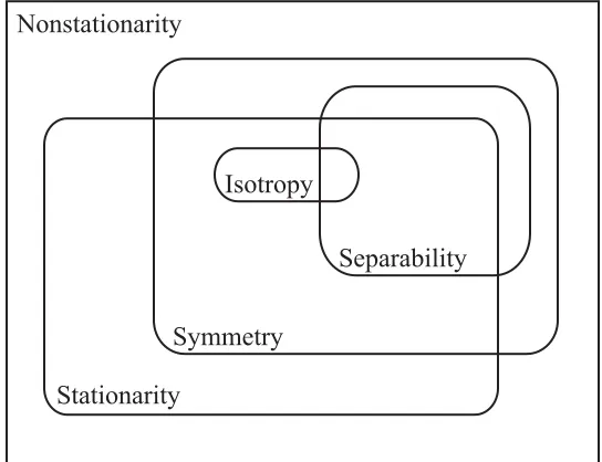
Now we visualize the relationship among separability, symmetry, stationarity
in the spatial-temporal setting. Figure 2.7 displays the Venn diagram describing
how these fundamental characteristics are mutually related to one another. As
one can see, symmetry and separability are mostly overlapped with stationarity
although separable covariance models (Fuentes et al. 2005) and symmetric ones
can be extended to nonstationary case. What is interesting here is that
separa-bility can possibly be a subset of symmetry, especially in terms of the covariance
function presented in (2.19). posssible expressions of a spectral density function
yielding a nonstationary symmetric covariance function are as follow:
or
fsj(ω;τ) =γjα2j +ω+τv12−νjβj2+ (τ +v2ω)2−νj,
where j = 1,· · · , k is the index of subregion satisfying stationarity, and sj is the center of thej-th subregion.
2.5
Real Application
In this section, we apply the class of asymmetric stationary spatial-temporal
covariance models to an air-pollution dataset, which is PM2.5 daily concentration aquired by the U.S. Environmental Protection Agency (EPA)’s Federal Reference
Method (FRM) monitoring stations. The main reason why we are interested in
PM2.5concentrations is that this air-pollutant is one of the important factors in the public health problem and, according to many environmenal studies, has complex
spatial or spatial-temporal dependency structure (Zidek (1997) and Golam Kibria
et al. (2002)). The spatial domain for this dataset is the northeastern U.S (Figure
2.8), which is almost the same region as the northeastern census division. The
measurements were obtained from August 1st to August 31st, 2003. First we
remove spatial trend by considering the second order polynomial function with
geodesic distances transformed from the orginal longitudes and latitudes in order
to take the earth’s curvature into account.
Now we briefly introduce the weighted least squares (WLS) estimation method
−80 −78 −76 −74 −72
36
38
40
42
44
46
longitude
latitude
Figure 2.8: The map of the 18 monitoring stations in the northeastern U.S.
Z(si, t) be the observed PM2.5 concentration for time t at site i; t = 1,· · · ,31, i= 1,· · · ,18, andX(s) andY(s) be the geodesic distances with unit of kilometers.
Then we consider the spatial-temporal structure as follows:
Z(si, t) = g(X(si), Y(si)|δ) +(si, t),
where g is the second-order polynomial function with coefficient parameters δ,
∼ M N(0, σI+Σ(θ)), σ is the nugget effect, and θ = (φ, α, β,v1,v2), where
φ is a partial sill. The variance-covariance matrix Σ(θ) is based on the following
Gaussian covariance functions:
M.1 C0(h;u) = φexpα2h2+β2u2
M.3 Cv2(h;u) = φexpα2h−uv22+β2u2
M.4 Cv(h;u) = φ
1−v1v2 exp
(1−v1v2)−2 α2h−uv22+β2(u−v1h)2
!
.
In order to estimate the covariance parameters, Θ = (σ,θ), we propose the empirical spatial-temporal semivariogram, γ(h(p, q);u) given by
γ(h(p, q);u)≡ 1 N(h(p, q);u)
(i,j,t,t∗)∈N(h(p,q);u)
Z(si, t)−Z(sj, t∗)
!2
, (2.25)
where
N(h(p, q);u)≡ {(i, j, t, t∗) :si−sj ∈ T(h(p, q));|t−t∗|=u},
{h(p, q)}={−h1(P),· · ·,−h1(1),0,· · · , h1(P)}
× {−h2(Q),· · · ,−h2(1),0,· · · , h2(Q)},
andZ(s, t) = Z(s, t)−g X(s), Y(s)|δ
!
andδ is the oridinary least squares (OLS)
estimator. HereT(h(p, q)) is prespecified tolerance region with centroid ofh(p, q).
Then the weighted-least squares (WLS) method (see Cressie (1993), pp.96) based
on the empirical semivariogram in (2.25) is employed to obtain the estimates of
the covariance parameters,Θ, which minimize the weighted sum of squares error
(WSSE), which is defined as
W(Θ)≡ P
p=−P Q
q=−Q U
u=0
|N(h(p, q);u)|
γ(h(p, q);u) γ(h(p, q);u|Θ) −1
2
, (2.26)
where γ(h(p, q);u|Θ) is the theoretical spatial-temporal semivariogram with
indicator function. We also consider the maximum likelihood (ML) estimation
method for obtaining the covariance parameter estimates.
Now we explain the result from the analysis of PM2.5 daily concentration dataset. The parameter estimation methods are performed with the spatially
detrended PM2.5 concentrations, {Z(s, t)}. In order to gain some computational benefit, we employ the estimates from the WLS method as initial values for
ob-taining the estimates from the ML method. The WSSE in (2.26) and the negative
log-likelihood are minimized using the routine optim in R. The Table 2.2 shows
the estimates of Θ from the WLS and the ML methods for each model (seeM.1
through M.4). As one can see, there does not exist any big difference of
param-eter estimates between the estimation methods for all the models. The estimates
for the components of v1 in M.2 have the same signs as those of v2 in M.3
re-gardless of the estimation methods. What is interesting here is that the signs of
the estimates for the last two components,v21 and v22 inM.4are opposite to the
ones inM.3. One possible reason is that, as we mentioned before, the parameter
vectorsv1,v2andvcontrol the shape of a spatial-temporal covariance function as
well as symmetry or lack of symmetry inherent in spatial-temporal processes. So,
the shape of the asymmetric covariance function employed in M.4 is determined
by adjustments fromv11 and v21, and from v12 and v22. From the WSSE and the
negative log-likelihoods based on the estimates from the corresponding methods,
we can know that, as the number of parameters increases, the given dataset gets
of information citerion.
−80 −78 −76 −74 −72
36
38
40
42
44
46
longitude
latitude
(a) M.1
−80 −78 −76 −74 −72
36
38
40
42
44
46
longitude
latitude
(b) M.2
−80 −78 −76 −74 −72
36
38
40
42
44
46
longitude
latitude
(c) M.3
−80 −78 −76 −74 −72
36
38
40
42
44
46
longitude
latitude
(d) M.4
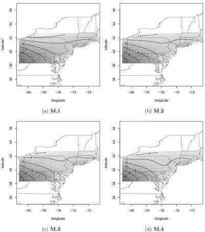
Figure 2.9: Kriging maps based on the ML estimates in Table 2.2 for each model. Note that the interpolation is performed at the regular grids on August 31, 2003.
Table 2.1: Square-root of mean squared prediction errors based on the WLS and the ML estimation methods at the two reserved stations.
Station M.1 M.2 M.3 M.4
WLS ML WLS ML WLS ML WLS ML
#1. 1.984 1.995 2.002 2.025 1.975 2.043 1.984 2.002
#2. 3.452 3.370 3.480 3.235 3.473 3.143 3.489 3.270
the prediction patterns are quite similar except portion of the region having the
negative predicted values. That is, M.2throughM.4can be preferred toM.1in
that only nonnegative PM2.5 concentrations are measured in pratice.
Now we evaluate the performances of the asymmetric spatial-temporal
co-variance models, M.1 through M.4 by means of the classical cross-validation
technique. We first remove two stations from the spatial domain of our interest,
analyze the data from the remaining stations, and compare the observed values
at the reserved stations with the predicted ones based on the estimation. Table
2.1 shows the square-root of mean squared prediction errors (RMSPE) at each
reserved station for every estimation method. In terms of the RMSPE, M.3 is
slightly better than the other asymmetric covariance models (M.2and M.4)
ex-cept the case of the ML estimation for the first reserved station although there is
no clear evidence that the general asymmetric covariance models (M.2-M.4)yield
more reliable predictions than the symmetric model (M.1), that is, the model
with v1 = v2 = 0. Based on the predictions from the classical cross-validation
values and the corresponding predicted values based on the ML estimates for
each reserved station. As one can see from these two figures, there is not any
big difference of the relationship between the observations and the corresponding
predictions among the covariance models and the prediction at the first reserved
station is done much better than the prediction at the second reserved station,
where every model produces slightly overestimated predicted values in comparison
to the observations.
In this section, we have applied a new class of asymmtric spatial-temporal
co-variance models to the PM2.5 daily concentrations at the FRM monitoring stations in the northeastern U.S. From the data analysis, we can know that the
spatial-temporal processes based on asymmetric covariance functions explain the given
dataset better than the process based on simple covariance function in terms of
the WSSE and the likelihood whereas, for the performance of prediction matter,
the number of stations is not enough for an asymmetric covariance function to
capture the spatial-temporal dependency structures.
2.6
Discussion
In this chapter, we introduced new concepts of symmetry in spatial-temporal
processes and proposed classes of asymmetric stationary spatial-temporal
covari-ance models. Since these covaricovari-ances are just Fourier transformations of the
definite. Unlike a process with separable, even nonseparable covariance, an
asym-metric spatial-temporal proecess is influenced by spatial-temporal dependencies,
which are mainly controled by asymmetry parameters. This characteristic is very
helpful to analyze the air-pollution data affected by some external metheological
conditions, for instance, wind speed, wind direction, air pressure and so on.
The asymmetric covariance models can be extended to the spatial domain with
d >2 although our results presented in this study are based on the two dimensional
spatial domain. For example, in case of spatial domain with longitude, latitude
and altitude, the asymmetric covariance models are constructed inR3×R. As part of our further research, we are estimating the parameters by means of Bayesian
Table 2.2: Parameter Estimates based on Gaussian Asymmetric Spatial-Temporal Covariance from WLS and ML methods. Note that (−4)≡10−4.
Θ
M.1 M.2 M.3 M.4
WLS ML WLS ML WLS ML WLS ML
σ 5.920 5.935 6.046 5.748 5.637 5.111 5.517 4.259
φ 105.7 105.3 106.5 105.3 105.5 105.5 103.2 109.2
α 0.003 0.003 0.003 0.004 0.003 0.004 0.003 0.005
β 0.838 0.888 0.842 0.847 0.826 0.800 0.821 0.978
v11 6.(-4) 1.(-4) 1.(-3) 2.(-3)
v12 -6.(-4) -3.(-4) -1.(-3) 1.(-3)
v21 20.07 20.07 -59.84 -59.82
v22 -45.10 -45.10 -59.98 -59.81
WSSE 686.1 641.1 678.8 580.4
5 10 15 20 25 30 35 40 5 1 01 52 02 53 03 54 0 predicted values observed value (a) M.1
5 10 15 20 25 30 35 40
5 1 01 52 02 53 03 54 0 predicted values observed value (b) M.2
5 10 15 20 25 30 35 40
5 1 01 52 02 53 03 54 0 predicted values observed value (c) M.3
5 10 15 20 25 30 35 40
5 1 01 52 02 53 03 54 0 predicted values observed value (d) M.4
Chapter 3
Testing Lack of Symmetry in
Spatial-Temporal Processes
3.1
Introduction
Symmetry and separability are the main assumptions used in spatial statistics
about a covariance function. Symmetry and separability in spatial or
spatial-temporal processes are highly related to each other. Separability provides many
advantages, such as the simplified representation of the covariance matrix and,
consequently, important computational benefits. Symmetry is related to the
spa-tial or spaspa-tial-temporal dependencies. This characteristic has been assumed
be-cause of mathematical convenience, modeling parsimony or calculational efficiency.
The common advantage of symmetry and separability is the simplification attained
for modeling purpose. However, many studies in environmental sciences show that