Volume 2007, Article ID 41679,7pages doi:10.1155/2007/41679
Research Article
Duct Modeling Using the Generalized
RBF Neural Network for Active Cancellation of
Variable Frequency Narrow Band Noise
Hadi Sadoghi Yazdi,1Javad Haddadnia,1and Mojtaba Lotfizad2
1Engineering Department, Tarbiat Moallem University of Sabzevar, P.O. Box 397, Sabzevar, Iran 2Department of Electrical Engineering, Tarbiat Modarres University, P.O. Box 14115-143, Tehran, Iran
Received 27 April 2005; Revised 1 February 2006; Accepted 30 April 2006
Recommended by Shoji Makino
We have shown that duct modeling using the generalized RBF neural network (DM RBF), which has the capability of modeling the nonlinear behavior, can suppress a variable-frequency narrow band noise of a duct more efficiently than an FX-LMS algorithm. In our method (DM RBF), at first the duct is identified using a generalized RBF network, after thatN stage of time delay of the input signal to theNgeneralized RBF network is applied, then a linear combiner at their outputs makes an online identification of the nonlinear system. The weights of linear combiner are updated by the normalized LMS algorithm. We have showed that the proposed method is more than three times faster in comparison with the FX-LMS algorithm with 30% lower error. Also the DM RBF method will converge in changing the input frequency, while it makes the FX-LMS cause divergence.
Copyright © 2007 Hindawi Publishing Corporation. All rights reserved.
1. INTRODUCTION
In the recent years, acoustic noise canceling by active meth-ods, due to its numerous applications, has been in the fo-cus of interest of many researches. Contrary to the passive method, it is possible using the active method to suppress or reduce the noise in a small space particularly in low frequen-cies (below 500 Hz) [1,2]. Active noise control was intro-duced for the first time by Paul Lveg in 1936 for suppressing the noise in a duct [3]. In the active control method by pro-ducing a sound with the same amplitude but with opposite phase, the noise is removed. For this purpose, the amplitude and phase of a noise must be detected and inverted. The de-veloped system must have the adaptive noise control capabil-ity [3]. In usual manner, an FIR filter is used in ANC whose weights are updated by a linear algorithm [4,5]. Using the linear algorithm of LMS is not possible due to the nonlinear environment of the duct and the appearing of the secondary path transfer functionH(z). Hence, the FX-LMS algorithm is presented in which the filtered input noisex(n) is used as an input to the algorithm [6,7]. The notable points in ANC are as follows.
(i) The duct length and the distance between the system elements are such that the system becomes causal [8].
(ii) Regarding the speaker response, no decrease will be obtained in frequencies below 200 Hz [2]. Also passive techniques for reducing the noise in frequencies below 500 Hz have not been successful [1,2]. Therefore, the ANC systems are used in the range of 200 to 500 Hz and above 500 Hz.
The existence of nonlinear effects in ANC complicates the use of the linear algorithm FX-LMS and similar algorithms. Di-vergence or slow conDi-vergence is among these difficulties. For this purpose, identification systems with a nonlinear struc-ture are used where a neural network is among these solu-tions [9–11]. The radial basis function (RBF) networks are used in processing temporal signals for radar [12], in the predictor filter in position estimation from present and past samples [13], and in adaptive prediction and control [14,15]. Buffering data, feedback from the output of the system, and state machines are used in modeling temporal signals. In time delay RBF neural networks, also, by buffering data [16], and using the feedback from the output in the recurrent RBF (RRBF) [17], this work is accomplished.
c(z) W(z)
LMS
H(z)
x¼( n) x(n)
y(n) y¼( n)
e(n) L
ANC controller Input microphone
Primary noise Noise source
Canceling speaker
Error microphone
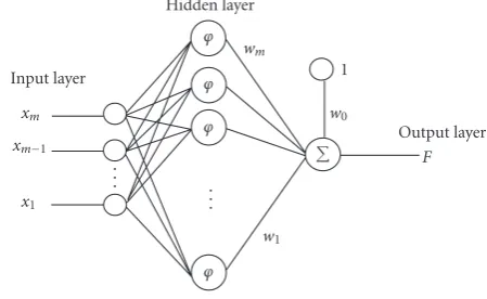
Figure1: Using the FX-LMS algorithm in a single channel ANC system.
x(n−N+ 1) are fed toNgeneralized RBF neural networks and then the linear combination of their outputs is used for canceling the acoustic noise inside a duct. For precise sim-ulation of the proposed algorithm and comparison to the conventional FX-LMS method, the transfer function of the primary path (the duct transfer function) and the secondary path must be available, which for this purpose, the informa-tion given in [18] which is obtained practically is utilized.
Section 2of this paper concerns the investigation of the active noise control in a duct and the FX-LMS algorithm. Section 3 contains a short review of the RBF and general-ized RBF neural networks. InSection 4, the proposed system and its application in ANC are presented and inSection 5the conclusions are presented.
2. PRINCIPLE OF ACTIVE NOISE CONTROL IN A DUCT
If we assume the noise propagates in a one-dimensional form, then it is possible to use a single channel ANC for noise cancellation. For simulation and implementation of this system, a narrow duct is used as inFigure 1. According toFigure 1, the primary noise before reaching to the speaker is picked up by the input microphone. The system uses the input signal for generating the noise canceling signal y(n). The generated sound by the speaker gives rise to a reduc-tion in the primary noise. The error microphone measures the remaining signale(n) which can be minimized using an adaptive filter which is used for identifying the duct’s transfer function. Because of using the input and error microphones, we must consider some functions which are known as the secondary path effects. In such a system, usually for cancel-ing the noise, the FX-LMS algorithm,Figure 1, and (1) are considered [1,19–21]. The vectorx(n) is a filtered copy of the vectorx(n).
Wn+1=Wn−μenXn, (1)
whereenis the residual signal andWn =[wn(1),wn(2),. . .,
wn(M)]Tis the weight vector of the estimator of lengthM.
xm
xm 1
x1
. . . Input layer
Hidden layer ϕ
ϕ
ϕ
. . .
ϕ wm
w1 1 w0
F Output layer
Figure2: Structure of an RBF network.
InFigure 1, thec(z) is an estimation ofH(z) which can be obtained by some offline techniques [22]. The considerable points in the execution the FX-LMS are the following.
(i) Canceling the broadband noise needs a filter of high order which increases the duct length [22].
(ii) In order to choose the proper stepsize, we need the knowledge of statistical properties of the input data [23,24].
(iii) To ensure the convergence, the stepsize is chosen small; hence the convergence speed will be low and the per-formance will be weak.
(iv) For executing the above algorithm, we need to estimate the secondary path.
(v) This algorithm is only applicable to a linear controller and is not either suitable for nonlinear controllers or it is slow. For modeling the nonlinear behavior of this system, neural networks can be employed.
3. THE RBF NEURAL NETWORKS
The RBF networks usually have three layers as shown in Figure 2. The first layer comprises the input nodes, the sec-ond layer, which is a hidden layer, includes a nonlinear trans-formation, and the third layer includes the output layer. The output in terms of the input is given by
Fj(x)=
r
i=1
wi jϕix−ci,δi
, (2)
x(n)
x 1 x(n 1) x 1 x(n 2)
x
1 x(n N)
GRBF GRBF GRBF GRBF
f0 α0
f1 α1
f2 α2
fN αN
LMS
+
+ + + F +
d(n)
Figure3: Structure of the proposed method.
3.1. The generalized RBF neural network
In this paper, the generalized neural network is used for mod-eling the duct. In this type of RBF, theϕi(x) function is com-puted as [25]
ϕi(x)=Gx−ci=exp
−1
2
x−ci
T−1x−c
i
,
(3)
whereis the covariance matrix of the input data andciare the centers of the Gaussian functions. The optimum weight vector is obtained as
W =GTG−1GTd, (4)
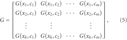
where d is the desired value and G is the Green func-tion which for kinputsx1 to xk and Gaussian centersc =
[c1,. . .,cm], its Green Function is as follows:
G=
⎡ ⎢ ⎢ ⎢ ⎢ ⎢ ⎢ ⎣
Gx1,c1
Gx1,c2
· · · Gx1,cm
Gx2,c1
Gx2,c2
· · · Gx2,cm
..
. ... ...
Gxk,c1
Gxk,c2
· · · Gxk,cm
⎤ ⎥ ⎥ ⎥ ⎥ ⎥ ⎥ ⎦
, (5)
wherexkis thekth learning sample.
4. THE PROPOSED ALGORITHM
The time delay neural network presented in this paper in-cludesNstages which are illustrated inFigure 3. At first, the duct is identified by the generalized RBF, GRBF, and then the results are combined by a linear adaptive filter such as LMS. Because of changing space with GRBF, obtaining error will be less than input space or the MSE at Φ-space is smaller than the input space; so we expect LMS has had smaller er-ror without converting space. This subject has been proved in the appendix.
The relation between the output and the input is given in
F=
N
j=0
αj·fj
x(n−j),
F=
N
j=0
αj
m
i=1
wiGx(n−j)−ci
,
(6)
whereNis the number of the delayed input signal samples andmis the number of the used kernels in the generalized RBF network.wis are obtained from (4) andαjs are updated with LMS algorithm according to
An+1=An−2μ·Yn·en, (7)
where An = [αn(1),αn(2),. . .,αn(N)]T, Yn = [fn(1),
fn(2),. . .,fn(N)]T, and en is the system error which is
ob-tained from subtracting the system output, Ffrom the de-sired value of the signal,dnat instantn. In noise reduction problem, anddnis the primary noise which reaches the exci-tation speaker.
4.1. Applying the proposed algorithm in
active noise canceling
The present network is used to active noise cancel as in Figure 4. At instant two points are interested in the proposed system as
(a) deletion of secondary path estimationc(z),
(b) learning the transfer function of GRBF and the linear-ity of active noise control system using this idea.
In the next subsections duct modeling and noise cancel-lation are explained.
4.2. Duct system function identification
x(n)
H(z)
y(n) e(n) L
Input microphone
Primary noise Noise source
Cancelling speaker
Error microphone The proposed
algorithm
Figure4: A structure for noise canceling in a duct by the proposed method.
Gaussian kernels of the GRBF function are computed using (9), (4.2).
ϕi(x)=Gx−ci=exp
− 1
2σi
x−ci2
, (8)
σi=
k1
m=1
xm−ci
2
k1−1
, (9)
xm=
xk|μik> μjk, j={1, 2,. . .,r} − {i}, k={1,. . .,N}
, (10)
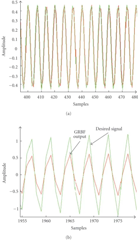
whereμikis the degree of membership of the patternsxkto theith group andμjkis the degree of membership to the jth group. In (4.2), the samples whose degrees of membership to theith group are more than other centers are attributed to that cluster and their standard deviations are considered as the Gaussian kernel standard deviation. The result of exe-cuting the generalized RBF on a sinusoidal chirp signal with a variable frequency of 300 to 305 Hz is shown inFigure 5. As shown inFigure 5(a), the output and the desired value in response to the narrow band signal has lower error, but this network is not able to learn the duct output in the broad-band spectrum of the input signal ofFigure 5(b), while the proposed algorithm gives better results.
Two networks are compared inFigure 6. The error norm of the proposed algorithm compared to the GRBF in duct identification is improved 94%. Hence, in identifying a sys-tem, the proposed system can be utilized. Several reasons can be mentioned for superiority of this system relative to the GRBF as follows.
(a) Using a filter bank instead of filter.
(b) UsingN buffered samples of data instead of a single stream of data.
(c) General and local consideration of data, that is, buffered data.
(d) Increasing the network capacity by increasing theα coefficient.
400 410 420 430 440 450 460 470 480 Samples
0.4 0.3 0.2 0.1 0 0.1 0.2 0.3 0.4 0.5
A
m
plitude
(a)
1955 1960 1965 1970 1975
Samples 1
0.5 0 0.5 1
A
m
plitude
GRBF output
Desired signal
(b)
Figure5: Part of the GRBF output and duct output in response to a sinusoidal chirp signal with a variable frequency (a) 300 to 305 Hz, (b) 200 to 500 Hz.
4.3. Active noise cancellation using
the proposed algorithm
After identifying the duct with the GRBF network, we pro-ceed canceling the noise in the duct by the structure pre-sented inFigure 3. The learning curve of the execution result on variable chirp sinusoid of 300–305 Hz for the proposed network in comparison to the FX-LMS algorithm is given in Figure 7.
1540 1545 1550 1555 1560 1565 Samples
0.8 0.6 0.4 0.2 0 0.2 0.4 0.6 0.8
A
m
plitude
GRBF output Desired and output of
proposed system
(a)
0 200 400 600 800 1000 1200 1400 1600 1800 Samples
250 200 150 100 50 0
L
ear
ning
cur
ve
Error (dB)
(b)
Figure 6: (a) Comparison of the RBF network output and the proposed algorithm in identifying the duct in response to a sinu-soidal chirp input of variable frequency 200–500 Hz. (b) The learn-ing curve of the proposed algorithm in duct identification.
5. CONCLUSIONS
The process of canceling the acoustic noise in a duct has a nonlinear nature. Therefore, linear adaptive filters such as LMS are not able to actively cancel the noise. Due to the good tracking capability of the LMS filter in a noisy environment, the FX-LMS has been presented as a basic method in ANC which models some what the nonlinear nature of the duct. In this paper, by modeling the duct using the generalized RBF neural network, it is possible to suppress the narrow band variable frequency noise in the duct in a better way than the FX-LMS method. The proposed method in comparison to the FX-LMS algorithm is more than three times faster and has 30% less error. Also, the change in the input frequency
0 500 1000 1500 2000 2500
Samples 250
200 150 100 50 0
L
ear
ning
cur
ve
Error (dB)
FX-LMS algorithm
The proposed method
Figure7: The learning curve to sinusoidal chirp with variable fre-quency of 300 to 305 Hz for the proposed system and the FX-LMS algorithm.
causes the divergence, which the proposed method converges as well.
In the proposed method, first the duct is identified by the GRBF neural network and using a linear adaptive combiner at their outputs, online identification of the nonlinear system becomes possible. The weights of the linear combiner are up-dated using the normalized LMS algorithm.
APPENDIX
Theorem A.1. Assume thatMSEi=E{e2}is the mean-square
error in the input space, then the MSE at Φ-space will be smaller than the input space.
Proof. the mapping is according to
Y=Φ(X), (A.1)
where Φ(X) = [ϕ(x,c1),ϕ(x,c2),. . .,ϕ(x,cK)] and we can assume thatϕ(x,ci) =exp(−(x−ci)2/2σ2). In simple form we can write ϕ(x,ci) = exp(−x2). By substituting e(k) =
xm(k)−x(k) inϕ(x,ci),xm(k) is the actual state of the sig-nal, then we have
ϕx(k),ci
=exp−x(k)2=exp−x
m(k) +e(k)
2
=exp−xm(k)2
exp−em(k)2
exp−2em(k)xm(k)
. (A.2)
Assuming em(k) is small enough, we can betake exp(−em(k)2) term. Also we know that exp(−xm(k)2) is the desired output in each dimension at theΦ-space. For simpli-fication, we substitutey=ϕ(x(k),ci), thus we have
y=ymexp
−2em(k)xm(k)
whereym=e(−xm(k)2). The Taylor series expansion of term exp(−2em(k)xm(k)) is
exp−2em(k)xm(k)
∼
=1−2em(k)xm(k),
y=ym−2emxmym=ym−2emxme−x
2
m=ym−αem.
(A.4)
The termα=2xme−x 2
mis always smaller than one, oreΦ=
αem, thus we have
MSEΦ=Ee2
Φ=α2Ee2, MSEΦ=α2MSEi.
(A.5)
The above equation shows that MSEΦ <MSEior“MSE
in Φ-space is smaller thanMSEin the input space.”
REFERENCES
[1] S. M. Kuo and D. R. Morgan, “Active noise control: a tutorial review,”Proceedings of the IEEE, vol. 87, no. 6, pp. 943–973, 1999.
[2] L. J. Eriksson, M. C. Allie, and R. A. Greiner, “The selection and application of an IIR adaptive filter for use in active sound attenuation,”IEEE Transactions on Acoustics, Speech, and Sig-nal Processing, vol. 35, no. 4, pp. 433–437, 1987.
[3] L. J. Eriksson and M. C. Allie, “System considerations for adaptive modelling applied to active noise control,” in Proceed-ings of IEEE International Symposium on Circuits and Systems (ISCAS ’88), vol. 3, pp. 2387–2390, Espoo, Finland, June 1988. [4] M. Bouchard and Y. Feng, “Inverse structure for active noise control and combined active noise control/sound reproduc-tion systems,”IEEE Transactions on Speech and Audio Process-ing, vol. 9, no. 2, pp. 141–151, 2001.
[5] S. J. Elliott and P. A. Nelson, “Active noise control,”IEEE Signal Processing Magazine, vol. 10, no. 4, pp. 12–35, 1993.
[6] D. R. Morgan, “An analysis of multiple correlation cancellation loops with a filter in the auxiliary path,”IEEE Transactions on Acoustics, Speech, and Signal Processing, vol. 28, no. 4, pp. 454– 467, 1980.
[7] J. C. Burgess, “Active adaptive sound control in a duct: a com-puter simulation,”Journal of the Acoustical Society of America, vol. 70, no. 3, pp. 715–726, 1981.
[8] B. Rafaely, J. Carrilho, and P. Gardonio, “Novel active noise-reducing headset using earshell vibration control,”Journal of the Acoustical Society of America, vol. 112, no. 4, pp. 1471– 1481, 2002.
[9] M. Bouchard, B. Paillard, and C. T. Le Dinh, “Improved train-ing of neural networks for the nonlinear active control of sound and vibration,”IEEE Transactions on Neural Networks, vol. 10, no. 2, pp. 391–401, 1999.
[10] L. S. H. Ngia and J. H. Sjoberg, “Efficient training of neu-ral nets for nonlinear adaptive filtering using a recursive Levenberg-Marquardt algorithm,”IEEE Transactions on Signal Processing, vol. 48, no. 7, pp. 1915–1927, 2000.
[11] S. D. Snyder and N. Tanaka, “Active control of vibration us-ing a neural network,”IEEE Transactions on Neural Networks, vol. 6, no. 4, pp. 819–828, 1995.
[12] T. Wong, T. Lo, H. Leung, J. Litva, and E. Bosse, “Low-angle radar tracking using radial basis function neural network,”IEE Proceedings F: Radar and Signal Processing, vol. 140, no. 5, pp. 323–328, 1993.
[13] N. E. Longinov, “Predicting pilot look-angle with a radial ba-sis function network,”IEEE Transaction on Systems, Man, and Cybernetics, vol. 24, no. 10, pp. 1511–1518, 1994.
[14] S. Clen, “Nonlinear time series modelling and prediction us-ing Gaussian RBF networks with enhanced clusterus-ing and RLS learning,”Electronics Letters, vol. 31, no. 2, pp. 117–118, 1995. [15] E. S. Chng, S. Chen, and B. Mulgrew, “Gradient radial basis function networks for nonlinear and nonstationary time se-ries prediction,”IEEE Transactions on Neural Networks, vol. 7, no. 1, pp. 190–194, 1996.
[16] M. R. Berthold, “A time delay radial basis function network for phoneme recognition,” inProceedings of IEEE International Conference on Neural Networks, vol. 7, pp. 4470–4472, 4472a, Orlando, Fla, USA, June-July 1994.
[17] Z. Ryad, R. Daniel, and Z. Noureddine, “The RRBF. Dynamic representation of time in radial basis function network,” in Proceedings of 8th IEEE International Conference on Emerging Technologies and Factory Automation (ETFA ’01), vol. 2, pp. 737–740, Antibes-Juan les Pins, France, October 2001. [18] B. Sayyarrodsari, J. P. How, B. Hassibi, and A. Carrier, “An
estimation-based approach to the design of adaptive IIR fil-ters,” inProceedings of the American Control Conference, vol. 5, pp. 3148–3152, Philadelphia, Pa, USA, June 1998.
[19] P. Lveg, “Process of silencing sound oscillations,” US Patent no. 2043416, June, 1936.
[20] E. Bjarnason, “Analysis of the filtered-X LMS algorithm,”IEEE Transactions on Speech and Audio Processing, vol. 3, no. 6, pp. 504–514, 1995.
[21] M. Rupp, “Saving complexity of modified filtered-X-LMS and delayed update LMS algorithms,”IEEE Transactions on Circuits and Systems II: Analog and Digital Signal Processing, vol. 44, no. 1, pp. 57–60, 1997.
[22] S. M. Kuo, I. Panahi, K. M. Chung, T. Horner, M. Nadeski, and J. Chyan, “Design of active noise control systems with the TMS320 family,” Tech. Rep. SPRA042, Texas Instruments, Dal-las, Tex, USA, 1996.
[23] S. K. Phooi, M. Zhihong, and H. R. Wu, “Nonlinear active noise control using Lyapunov theory and RBF network,” in Proceedings of the IEEE Workshop on Neural Networks for Signal Processing, vol. 2, pp. 916–925, Sydney, NSW, Australia, De-cember 2000.
[24] D. A. Cartes, L. R. Ray, and R. D. Collier, “Lyapunov turning of the leaky LMS algorithm for single-source, single-point noise cancellation,”Mechanical System and Signal Processing, vol. 17, no. 5, pp. 925–944, 2003.
[25] S. Haykin, Neural Networks: A Comprehensive Foundation, MacMillan College, New York, NY, USA, 1994.
Hadi Sadoghi Yazdiwas born in Sabzevar, Iran, in 1971. He received the B.S. degree in electrical engineering from Ferdosi Mashad University of Iran in 1994, and then he re-ceived to the M.S. and Ph.D. degrees in electrical engineering from Tarbiat Modar-res University of Iran, Tehran, in 1996 and 2005, respectively. He works in Engineering Department as Assistant Professor at Tar-biat Moallem University of Sabzevar. His
Javad Haddadnia works as an Assistant Professor at Tarbiat Moallem University of Sabzevar. He received the M.S. and Ph.D. degrees in electrical engineering from Amir Kabir University of Iran, Tehran, in 1999 and 2002, respectively. His research interests include image processing.
Mojtaba Lotfizadwas born in Tehran, Iran, in 1955. He received the B.S. degree in elec-trical engineering from Amir Kabir Univer-sity of Iran in 1980 and the M.S. and Ph.D. degrees from the University of Wales, UK, in 1985 and 1988, respectively. He joined the engineering faculty of Tarbiat Modarres University of Iran. He has also been a Con-sultant to several industrial and government organizations. His current research interests