Automatic Speechreading with Applications
to Human-Computer Interfaces
Xiaozheng Zhang
Center for Signal and Image Processing, Georgia Institute of Technology, Atlanta, GA 30332-0250, USA Email: [email protected]
Charles C. Broun
Motorola Human Interface Lab, Tempe, AZ 85284, USA Email: [email protected]
Russell M. Mersereau
Center for Signal and Image Processing, Georgia Institute of Technology, Atlanta, GA 30332-0250, USA Email: [email protected]
Mark A. Clements
Center for Signal and Image Processing, Georgia Institute of Technology, Atlanta, GA 30332-0250, USA Email: [email protected]
Received 30 October 2001 and in revised form 31 July 2002
There has been growing interest in introducing speech as a new modality into the human-computer interface (HCI). Motivated by the multimodal nature of speech, the visual component is considered to yield information that is not always present in the acoustic signal and enables improved system performance over acoustic-only methods, especially in noisy environments. In this paper, we investigate the usefulness of visual speech information in HCI related applications. We first introduce a new algorithm for automatically locating the mouth region by using color and motion information and segmenting the lip region by making use of both color and edge information based on Markov random fields. We then derive a relevant set of visual speech parameters and incorporate them into a recognition engine. We present various visual feature performance comparisons to explore their impact on the recognition accuracy, including the lip inner contour and the visibility of the tongue and teeth. By using a common visual feature set, we demonstrate two applications that exploit speechreading in a joint audio-visual speech signal processing task: speech recognition and speaker verification. The experimental results based on two databases demonstrate that the visual information is highly effective for improving recognition performance over a variety of acoustic noise levels.
Keywords and phrases:automatic speechreading, visual feature extraction, Markov random fields, hidden Markov models, poly-nomial classifier, speech recognition, speaker verification.
1. INTRODUCTION
In recent years there has been growing interest in introduc-ing new modalities into human-computer interfaces (HCIs). Natural means of communicating between humans and computers using speech instead of a mouse and keyboard provide an attractive alternative for HCI.
With this motivation much research has been carried out in automatic speech recognition (ASR). Mainstream speech recognition has focused almost exclusively on the acoustic signal. Although purely acoustic-based ASR systems yield ex-cellent results in the laboratory environment, the recogni-tion error can increase dramatically in the real world in the
presence of noise such as in a typical office environment with ringing telephones and noise from fans and human conver-sations. Noise robust methods using feature-normalization algorithms, microphone arrays, representations based on hu-man hearing, and other approaches [1, 2, 3] have limited success. Besides, multiple speakers are very hard to separate acoustically [4].
especially in acoustically hostile environments. In human speechreading, many of the sounds that tend to be difficult for people to distinguish orally are easier to see (e.g., /p/, /t/, /k/), and those sounds that are more difficult to distinguish visually are easier to hear (e.g., /p/, /b/, /m/). Therefore, vi-sual and audio information can be considered to be comple-mentary to each other [5, 6].
The first automatic speechreading system was developed by Petajan in 1984 [7]. He showed that an audio-visual sys-tem outperforms either modality alone. During the follow-ing years various automatic speechreadfollow-ing systems were de-veloped [8, 9] that demonstrated that visual speech yields information that is not always present in the acoustic sig-nal and enables improved recognition accuracy over audio-only ASR systems, especially in environments corrupted by acoustic noise and multiple talkers. The two modalities serve complementary functions in speechreading. While the audio speech signal is represented by the acoustic waveform, the visual speech signal usually refers to the accompanying lip movement, tongue and teeth visibility, and other relevant fa-cial features.
An area related to HCI is personal authentication. The traditional way of using a password and PIN is cumbersome since they are difficult to remember, must be changed fre-quently, and are subject to “tampering.” One solution is the use of biometrics, such as voice, which have the advantage of requiring little custom hardware and are nonintrusive. How-ever, there are two significant problems in current generation speaker verification systems using speech. One is the diffi -culty in acquiring clean audio signals in an unconstrained environment. The other is that unimodal biometric models do not always work well for a certain group of the popula-tion. To combat these issues, systems incorporating the visual modality are being investigated to improve system robustness to environmental conditions, as well as to improve overall accuracy across the population. Face recognition has been an active research area during the past few years [10, 11]. However, face recognition is often based on static face im-ages assuming a neutral facial expression and requires that the speaker does not have significant appearance changes. Lip movement is a natural by-product of speech production, and it does not only reflect speaker-dependent static and dynamic features, but also provides “liveness” testing (in case an im-poster attempts to fool the system by using the photograph of a client or pre-recorded speech). Previous work on speaker recognition using visual lip features includes the studies in [12, 13].
To summarize, speech is an attractive means for a user-friendly human-computer interface. Speech not only con-veys the linguistic information, but also characterizes the talker’s identity. Therefore, it can be used for both speech and speaker recognition tasks. While most of the speech informa-tion is contained in the acoustic channel, the lip movement during speech production also provides useful information. These two modalities have different strengths and weaknesses and to a large extent they complement each other. By incor-porating visual speech information we can improve a purely acoustic-based system.
To enable a computer to perform speechreading or speaker identification, two issues need to be addressed. First, an accurate and robust visual speech feature extraction al-gorithm needs to be designed. Second, effective strategies to integrate the two separate information sources need to be de-veloped. In this paper, we will examine both these aspects.
We report an algorithm developed to extract visual speech features. The algorithm consists of two stages of visual analysis: lip region detection and lip segmentation. In the lip region detection stage, the speaker’s mouth in the video se-quence is located based on color and motion information. The lip segmentation phase segments the lip region from its surroundings by making use of both color and edge informa-tion, combined within a Markov random field framework. The key locations that define the lip position are detected and a relevant set of visual speech parameters are derived. By enabling extraction of an expanded set of visual speech fea-tures, including the lip inner contour and the visibility of the tongue and teeth, this visual front end achieves an increased accuracy in an ASR task when compared with previous ap-proaches. Besides ASR, it is also demonstrated that the visual speech information is highly effective over acoustic informa-tion alone in a speaker verificainforma-tion task.
This paper is organized as follows. Section 2 gives a re-view of previous work on extraction of visual speech features. We point out advantages and drawbacks of the various ap-proaches and illuminate the direction of our work. Section 3 presents our visual front end for lip feature extraction. The problems of speech and speaker recognition using visual and audio speech features are examined in Sections 4 and 5, re-spectively. Finally, Section 6 offers our conclusions.
2. PREVIOUS WORK ON VISUAL FEATURE
EXTRACTION
It is generally agreed that most visual speech information is contained in the lips. Thus, visual analysis mainly focuses on lip feature extraction. The choice for a visual representation of lip movement has led to different approaches. At one ex-treme, the entire image of the talker’s mouth is used as a fea-ture. With other approaches, only a small set of parameters describing the relevant information of the lip movement is used.
In the image-based approach, the whole image contain-ing the mouth area is used as a feature either directly [14, 15], or after some preprocessing such as a principal components analysis [16] or vector quantization [17]. Recently, more so-phisticated data preprocessing has been used, such as a linear discriminant analysis projection and maximum likelihood linear transform feature rotation [18]. The advantage of the image-based approach is that no information is lost, but it is left to the recognition engine to determine the relevant fea-tures in the image. A common criticism of this approach is that it tends to be very sensitive to changes in illumination, position, camera distance, rotation, and speaker [17].
flow data were used as visual features. In [20], oral cavity features including width, height, area, perimeter, and their ratios and derivatives were used as inputs for the recognizer.
In more standard approaches, model-based methods are considered, where a geometric model of the lip contour is applied. The typical examples are deformable templates [21], “snakes” [22], and active shape models [23]. Either the model parameters or the geometric features derived from the shape such as the height and width of the mouth are used as fea-tures for recognition. For all three approaches, an image search is performed by fitting a model to the edges of the lips, where intensity values are commonly used. The diffi -culty with these approaches usually arises when the contrast is poor along the lip contours, which occurs quite often un-der normal lighting conditions. In particular, edges on the lower lip are hard to distinguish because of shading and re-flection. The algorithm is usually hard to extend to various lighting conditions, people with different skin colors, or peo-ple with facial hair. In addition, the teeth and tongue are not easy to detect using intensity-only information. The skin-lip and lip-teeth edges are highly confusable.
An obvious way of overcoming the inherent limitations of the intensity-based approach is to use color, which can greatly simplify lip identification and extraction. Lip fea-ture extraction using color information has gained interest with the increasing processing power and storage of hard-ware making color image analysis more affordable. However, certain restrictions and assumptions are required in existing systems. They either require individual chromaticity mod-els [24], or manually determined lookup tables [25]. More importantly, most of the methods only extract outer lip con-tours [26, 27]. No methods have been able to explicitly detect the visibility of the tongue and teeth so far.
Human perceptual studies [28, 29] show that more visual speech information is contained within the inner lip con-tours. The visibility of the teeth and tongue inside the mouth is also important to human lipreaders [30, 31, 32]. We, there-fore, aim to extract both outer and inner lip parameters, as well as to detect the presence/absence of the teeth and tongue. One of the major challenges of any lip tracking system is its robustness over a large sample of the population. We include two databases in our study. One is the audio-visual database from Carnegie Mellon University [33, 34] including ten test subjects, the other is the XM2VTS database [35, 36], which includes 295 test subjects. In the next section, we present an approach that extracts geometric lip features us-ing color video sequences.
3. VISUAL SPEECH FEATURE EXTRACTION
3.1. Lip region/feature detection
3.1.1 Color analysis
The RGB color model is most widely used in computer vision because color CRTs use red, green, and blue phosphors to create the desired color. However, its inability to separate the luminance and chromatic components of a color hinders the effectiveness of color in image recognition. Previous studies
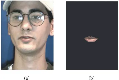
(a) (b)
Figure1: (a) Original image. (b) Manually extracted lip ROI.
[37, 38] have shown that even though different people have different skin colors, the major difference lies in the intensity rather than the color itself. To separate the chromatic and luminance components, various transformed color spaces can be employed, such as the normalized RGB space (which we denote as rgb in the following), YCbCr, and HSV. Many transformations from RGB to HSV are presented in the literature. Here the transformation is implemented after [39].
The choice of an appropriate color space is of great im-portance for successful feature extraction. To analyze the statistics of each color model, we build histograms of the three color components in each color space by discretizing the image colors and counting the number of times each dis-crete color occurs in the image. We construct histograms for the entire image and for the manually extracted lip regions of interest (ROI) bounded within the contour, as shown in Figure 1.
Typical histograms of the color components in the RGB, rgb, HSV, and YCbCr color spaces are shown in Figures 2, 3, 4, and 5, where two cases are given: (a) those for the entire image and (b) those for the extracted lip region only.
1 0.8
0.6 0.4
0.2 0
0 500 1000 1500
Histogram of R component for the entire image
1 0.8
0.6 0.4
0.2 0
0 5 10 15 20
Histogram of R component for the ROI
1 0.8
0.6 0.4
0.2 0
0 500 1000
1500 Histogram of G component for the entire image
1 0.8
0.6 0.4
0.2 0
0 5 10 15 20
Histogram of G component for the ROI
1 0.8
0.6 0.4
0.2 0
0 500 1000
1500 Histogram of B component for the entire image
(a)
1 0.8
0.6 0.4
0.2 0
0 5 10 15 20
Histogram of B component for the ROI
1 0.8
0.6 0.4
0.2 0
0 2000 4000 6000 8000 10000
12000 Histogram of r component for the entire image
1 0.8
0.6 0.4
0.2 0
0 50 100 150 200 250
Histogram of r component for the ROI
1 0.8
0.6 0.4
0.2 0
0 2000 4000 6000 8000 10000 12000
Histogram of g component for the entire image
1 0.8
0.6 0.4
0.2 0
0 50 100 150 200 250
Histogram of g component for the ROI
1 0.8
0.6 0.4
0.2 0
0 2000 4000 6000 8000 10000 12000
Histogram of b component for the entire image
(a)
1 0.8
0.6 0.4
0.2 0
0 50 100 150 200 250
Histogram of b component for the ROI
1 0.8
0.6 0.4
0.2 0
0 1000 2000 3000 4000 5000 6000
Histogram of H component for the entire image
1 0.8
0.6 0.4
0.2 0
0 50 100 150 200
Histogram of H component for the ROI
1 0.8
0.6 0.4
0.2 0
0 200 400 600 800 1000 1200 1400 1600 1800
Histogram of S component for the entire image
1 0.8
0.6 0.4
0.2 0
0 10 20 30 40 50
Histogram of S component for the ROI
1 0.8
0.6 0.4
0.2 0
0 200 400 600 800 1000
Histogram of V component for the entire image
(a)
1 0.8
0.6 0.4
0.2 0
0 5 10 15 20
Histogram of V component for the ROI
250 200
150 100
50 0
0 200 400 600 800 1000
Histogram of Y component for the entire image
250 200
150 100
50 0
0 5 10 15 20 25
Histogram of Y component for the ROI
250 200
150 100
50 0
0 1000 2000 3000 4000 5000
Histogram of Cb component for the entire image
250 200
150 100
50 0
0 20 40 60 80 100 120 140
Histogram of Cb component for the ROI
250 200
150 100
50 0
0 1000 2000 3000 4000 5000 6000
Histogram of Cr component for the entire image
(a)
250 200
150 100
50 0
0 10 20 30 40 50 60 70 80 90
Histogram of Cr component for the ROI
(a)
(b) (c)
(d) (e)
(f) (g)
Figure6: Lip region detection. (a) Gray level representation of the original RGB color image. (b) Hue image. (c) Binary image after H/S thresholding. (d) Accumulated difference image. (e) Binary image (d) after thresholding. (f) Result from AND operation on (c) and (e). (g) Original image with the identified lip region.
The first figure in Figure 4b shows the histogram of hue for the lip region. We observe that the red hue falls into two separate subsets at the low and high ends of the whole color range, as a result of the wrap-around nature of hue (hue is defined on a ring). For easy use of the hue component, we rotate the hue to the left, so that the red color falls in a connected region that lies at the high end of the hue range close to 1 (we scale the hue by a factor of 360 so that it is defined over the range [0,1]). The modified RGB to HSV conversion is shown in the following:
M=max(R,G,B)
m=min(R,G,B)
d=M−m
Value calculation:V=M
Saturation calculation:S=(M==0)?0 :d/M
Hue calculation: if (S==0)
H=0 else
if (d==0) d=1
H=(R==M)?((G−B)/d) : (G==M)?(2+(B−R)/d) : (4 + (R−G)/d)
H− =.2
H/=6
if (H <0) H+=1
3.1.2 Lip region detection
The problem of visual feature extraction consists of two parts: lip region detection and lip feature extraction. In the first stage of the visual analysis, the speaker’s mouth in the video sequence is located. We utilize hue for this purpose. Given an RGB image of the frontal view of a talker, as shown in Figure 6a, a modified hue color image can be derived (Figure 6b). Since the modified red hue value lies at the high end, the lips appear to be the brightest region, but there is
considerable noise in the hue image. Part of the noise is re-lated to the unfortunate singularity property of RGB to HSV conversion, which occurs when R=G=B (saturation=0) [40]. To remove this type of noise, we require thatSexceed a certain preset value. For segmenting the lips, we label a pixel as a lip pixel if and only ifH(i, j)> H0,S(i, j)> S0, where
H0=0.8,S0=0.25 forH, S∈[0,1]. The accuracies of those
two values are not very critical, and they proved to generalize well for other talkers. The resulting binary image is shown in Figure 6c.
Another component of the noise is caused by the non-lip red blobs in the image, for example when there are distract-ing red blobs in the clothdistract-ing, or if the person has a ruddy complexion, as is the case for the person shown in Figure 6. In this case, we exploit motion cues to increase the robust-ness of detecting the lips. In this approach, we search for the moving lips in the image if an audio signal is present in the acoustic channel. To detect the moving object, we build dif-ference images between subsequent frames and sum over a series of frames. The accumulated difference image (ADI) is defined as follows:
ADI0(i, j)=0,
ADIk(i, j)=ADIk−1(i, j) +∆Rk(i, j), k∈1, . . . , T,
(1)
where the difference image ∆Rk(i, j) is calculated by pixel-wise absolute subtraction between adjacent frames ∆Rk(i, j)= |Rk(i, j)−Rk−1(i, j)|. Note that we use the R
com-ponent for our lip detection.Tis set to 100 in our work, that is, we sum the difference images over 100 frames. An example of an accumulated difference image is shown in Figure 6d. To separate the moving lips from the background, we use two subsequent thresholding operations. The first threshold is applied to the entire image, where thresholdt1 is derived
(a) (b) (c)
Figure7: (a) Configuration of lip sites (◦) and edge sites (—). (b) Neighborhood system for lip sites. The filled circle represents the site, and unfilled circles represent the neighbors of the site. (c) Neighborhood system for horizontal edge sites. The thick line represents the site, and thin lines represent the neighbors of the site.
derived. The binary image based ont2is shown in Figure 6e
with moving mouth being highlighted. When this is com-bined with the binary image from the hue/saturation thresh-olding, shown in Figure 6c, the binary image, Figure 6f, is obtained by combining the two binary images using an AND operation. Based on the resulting image, we extract the lip re-gion from its surroundings by finding the largest connected region. The identified lip area is shown as a white bounding box in Figure 6g.
There exist many other sophisticated classifiers in the lit-erature such as in [42, 43]. The effectiveness of this rather simple algorithm lies in the fact that the hue color is very efficient in identifying the lips due to its color constancy and high discriminative power. It should be noted, however, that it is assumed here that the video sequence contains the frontal view of a speaker without significant head motion.
The lip location algorithm described above needs to be done only once for the first image of the sequence. For the succeeding frames, we estimate the lip region from the de-tected lip features of the previous frame based on the as-sumption that the mouth does not move abruptly from frame to frame. Subsequent processing is restricted to the identified lip region.
3.1.3 MRF-based lip segmentation
Since hue in [39] is defined on a ring (see Section 3.1.1) rather than on an intervalR, standard arithmetic operations do not work well with it. In [44] another hue definition was suggested,H = R/(R + G), where R, G denote the red and green components. It is defined onR, and achieves nearly as good a reduction of intensity dependence as the conventional hue definition.
In addition to the color information, edges characterize object boundaries and provide additional useful informa-tion. We perform edge detection by using a Canny detection on the hue image. In the Canny detector, the input imageH
is convolved with the first derivative of a Gaussian function
G(i, j)=σ2e−(i2+j2)/2σ2
(we setσ to 1.0 in our implementa-tion) to obtain an image with enhanced edges. The convo-lution with the two-dimensional Gaussian can be separated into two convolutions with one-dimensional Gaussians in di-rectionsiandj. The magnitude of the result is computed at
each pixel (i, j) as
e(i, j)=c1Hi(i, j)2+c2Hj(i, j)2, (2)
where Hi and Hj are results of the convolutions between
the first derivatives of the Gaussian and the imageHin the two separate directions. Based on this magnitude, a non-maximum suppression and double thresholding algorithm are performed and the edge map is derived. In expression (2),c1andc2are normally set to be equal. Since the lips
con-tain mainly horizontal edges, we assignc1 =10c2 to
accen-tuate the importance of horizontal edges. This modification results in an improved edge map for lip images.
To combine the edge and hue color information, we have chosen to use the machinery of the Markov random field (MRF), which has been shown to be suitable for the prob-lem of image segmentation. An MRF is a probabilistic model defined over a lattice of sites. The sites are related to each other through a neighborhood system. In MRFs, only neigh-boring sites have direct interaction with each other. Due to the Hammersley-Clifford theorem, the joint distribution of an MRF is equivalent to a Gibbs distribution, which takes the form
p(x)= 1 Zexp
−1 TU(x)
, (3)
whereZis the normalizing constant,Tthe temperature con-stant, andU(x) the Gibbs potential
U(x)=
c∈C
Vc(x), (4)
which is the sum of clique potentialsVc(x) over all possible cliquesC.
In our problem, each sites = (i, j) is assigned a label
xl
s=1 (for lips) or 0 (for non-lips), andxse=1 (for edge) or 0
The MAP estimate is equivalent to that found by minimizing the posterior energy term
x∗=arg min
x U
x|y, (5)
wherex= {xl,xe}denotes the configuration of the labeling,
andythe observed image data.
Using Bayes’ rule, the posterior probability is expressed as
px|y∝py|xlpy|xep(x), (6)
where p(y|xl) andp(y|xe) represent the conditional
proba-bility distribution of the observed image color and edge data given the true interpretation of the images xl andxe. They
are modeled as follows:
py|xl∝exp the image with the lip label xl
s. They are obtained by using
Otsu’s methods [41] based on the histogram. The observed color data is represented by the hue color ys=R/(R + G) at
wherees represents the strength of the edge at sitesand is the magnitude derived from the Canny detector described in (2). The labelxe
s is the edge label at sites. It is 1 if there is
an edge, and 0 otherwise. Since the edge map is defined for each pixel, we shift the edge map by 1/2 pixel downwards against the original image, so that xe
s ats = (i, j) indicates
the edge between pixels (i, j) and (i, j+ 1). For simplicity, we only consider horizontal edges.
By combining the above equations, it is clear that the MAP solution is equivalent to minimizing the following en-ergy function:
In (9), the first term expresses the prior expectation and the second and third terms bind the solution to the color and edge data, respectively. We useλ1 = 2 andλ2 = 1. TheVc
are the clique potentials describing the interactions between neighbors. They encode a priori knowledge about the spa-tial dependence of labels at neighboring sites. They are com-posed of three parts
Vc=k1Vcl+k2Vce+k3Vcle, (10)
wherek1=10,k2=1, andk3=1. The first term in (10),Vcl,
imposes smoothness and continuity of color regions over an
entire image, the second term,Ve
c, is responsible for
bound-ary organization for the edges, and the third term,Vle c, is the
coupling term between the color and edge labels. There has been some work on applying statistical methods to estimate parameters for the clique potentials, such as in [46, 47]. How-ever, choosing the clique potentials on an ad hoc basis has been reported to produce promising results [48, 49]. In this paper, we define these terms as follows:
Vl
For the optimization strategy, a stochastic relaxation technique, such as simulated annealing, can be used to find the globally optimal interpretation for the image [45]. How-ever, an exhaustive search for a global optimum imposes a large computational burden because the labels for all pix-els need to be estimated simultaneously. Therefore, alterna-tive estimates have been suggested, including using a Monte Carlo method [50], mean field technique [51], iterated con-ditional modes (ICM) [52], and high confidence first (HCF) algorithm [53]. We chose to use the HCF, because it is deter-ministic, computationally attractive, and achieves good per-formance. HCF differs from the other methods in the order of sites which are visited. Instead of updating the pixels se-quentially, HCF requires that the site that is visited next be the one that causes the largest energy reduction. This pro-cedure converges to a local minimum of the Gibbs potential within a relatively small number of cycles. The current lip feature extraction algorithm runs at a speed of 5 seconds per frame with an original image resolution of 720×480. The algorithm is designed to be scalable and can work in near-real time at lower image resolution with decreased tracking accuracy.
3.2. Visual speech features
Figure8: Segmented lips overlayed on the original image.
Figure9: Measured feature points on the lips.
w2
w1
h3
h2
h1
h4
Figure 10: Illustration of the extracted geometric features of the lips.
replace the old one with it. Finally, given the constraints of the outer corners and the upper/lower inner lip, we locate the inner lip corners. Examples of extracted feature points are shown in Figure 9.
Based on the extracted key feature points, we can derive the geometric dimensions of the lips. The following features are used in our study: mouth width (w2), upper/lower lip
width (h1, h3), lip opening height/width (h2, w1), and the
dis-tance between the horizontal lip line and the upper lip (h4).
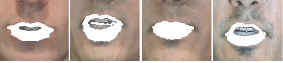
An illustration of the geometry is shown in Figure 10. Besides the geometric dimensions of the lips, we also detect the visibility of the tongue and teeth. For detecting the tongue, we search for the “lip” labels within the inner lip region. Two cases need to be differentiated, as shown in Figure 11. In the first case, the tongue is separated from the lips by the teeth. Tongue detection is trivial in this case. In the second case however, the tongue merges with the lips. From the segmented image, we have a lip closure case. Here, we use the gradient of the intensity to detect the inner upper/lower
(a) (b)
Figure11: (a) Tongue is separated from the lips. (b) Tongue merges with the lips.
lip. In the case that h2 = 0, we search for intensity
gradi-ent values along the vertical lip line. If the gradigradi-ents of two points exceeding a preset value are found, they are identi-fied as upper/lower inner lip. The parameter for the tongue is represented by the total number of lip-color pixels within the inner lip contour.
The teeth are also easy to detect since their H values are distinctly different from the hue of the lips. This is a big advantage compared with gray-level-based approaches that may confuse skin-lip and lip-teeth edges. Teeth are detected by forming a bounding box around the inner mouth area and testing pixels for white teeth color:S < S0, whereS0 =0.35.
The parameter of the teeth is the total number of white pixels within the bounding box.
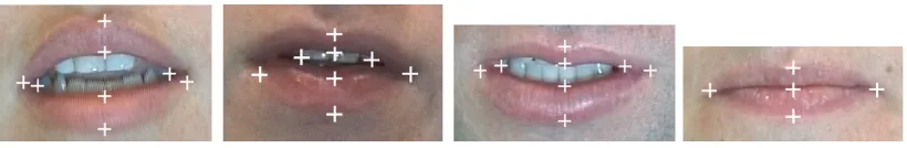
Figure12: Examples of detected feature points.
methods. In the geometric constraint method the ratio be-tween the lip opening height and the mouth width is less than a threshold, and in the time constraint method the variation of the measures between successive frames is within a limited range. Figure 12 shows examples of feature extraction results. Since the evaluation of feature extraction methods is often subjective, it is common that the direct evaluation is omit-ted at the visual feature level, and performance is evaluaomit-ted based only on the final results of the system, which could be a speech recognition or speaker verification system. In our experiment, we evaluate the accuracy of the derived visual features for the tongue and teeth by randomly selecting a set of test sequences. These sequences are typically hundreds of frames long. We verify the computed results by visual inspec-tion of the original images. The results show that the com-puted feature sets have an accuracy of 93% for the teeth and 91% for tongue detection, approximately.
4. AUTOMATIC SPEECH RECOGNITION
4.1. Visual speech recognition
In this section, we describe the modeling of the extracted lip features for speech recognition using hidden Markov models. HMMs [55] have been successfully used by the speech recog-nition community for many years. These models provide a mathematically convenient way of describing the evolution of time sequential data.
In speech recognition, we model the speech sequence by a first-order Markov state machine. The Markov property is encoded by a set of transition probabilities with ai j = P(qt = j|qt−1 = i), the probability of moving to state j
at time t given the state i at time t−1. The state at any given time is unknown or hidden. It can, however, be proba-bilistically inferred through the observations sequenceO =
{o1,o2, . . . ,oT}, whereot is the feature vector extracted at
time frametandT is the total number of observation vec-tors. The observation probabilities are commonly modeled as mixtures of Gaussian distributions
bj(o)= M
k=1
cjkᏺo;µjk,Σjk, (12)
whereMk=1cjk = 1 andM is the total number of mixture components, µjk andΣjk are the mean vector and covari-ance matrix, respectively, for thekth mixture component in state j.
An HMM representing a particular word class is defined by a parameter set λ = (A, B, π), where π is the vector of
initial state probabilities,A= {ai j}the matrix of state tran-sition probabilities, and B = {bi(ot)} the vector of
state-dependent observation probabilities. Given a set of training data (segmented and labeled examples of speech sequences), the HMM parameters for each word class are estimated using a standard EM algorithm [56]. Recognition requires evalu-ating the probability that a given HMM would generate an observed input sequence. This can be approximated by using the Viterbi algorithm. For isolated word recognition consid-ered in this paper, given a test tokenO, we calculateP(O|λi) for each HMM, and selectλcwherec=arg maxiP(O|λi).
We perform the speech recognition task using the audio-visual database from Carnegie Mellon University [33]. This database includes ten test subjects (three females, seven males) speaking 78 isolated words repeated ten times. These words include numbers, days of the week, months, and oth-ers that are commonly used for scheduling applications. Figure 13 shows a snapshot of the database.
We conducted tests for both speaker-dependent and in-dependent tasks using visual parameters only. The eight vi-sual features used are:w1,w2,h1,h2,h3,h4corresponding to
Figure 10, and the parameters for the teeth/tongue. The vi-sual feature vectors are preprocessed by normalizing against the average mouth widthw2of each speaker to account for
the difference in scale between different speakers and diff er-ent record settings for the same person. For comparison, we also provide test results on partial feature sets. In particular, we limited the features to the geometric dimensions of the inner contour (w1, h2), and outer contour (w2, h1+h2+h3).
The role of the use of the tongue and teeth parameters was also evaluated. For the HMM, we use a left-right model and consider continuous density HMMs with diagonal observa-tion covariance matrices, as is customary in acoustic ASR. We use ten states for each of the 78 HMM words and due to the training set size model the observation vectors using only two Gaussian mixtures for the speaker-independent task. Be-cause of an even more limited training data available, we use only one Gaussian mixture in the speaker-dependent case. The recognition system was implemented using the Hidden Markov Model Toolkit (HTK) [57].
Table1: Recognition rates for visual speech recognition using database [33]. The numbers represent the percentage of correct recognition.
Features SD (static) SD (static +∆) SI (static) SI (static +∆)
All (8) 45.51 45.59 18.17 21.08
All excl. tongue/teeth (6) 40.26 40.60 12.78 16.70 Outer/inner contour (4) 39.90 43.45 14.85 20.97 Outer contour (2) 28.72 35.16 7.9 12.55 Inner contour (2) 29.5 31.88 11.91 15.63
Anne Betty Chris Gavin Jay
Figure13: Examples of extracted lip ROI from the audio-visual database from Carnegie Mellon University [33].
times, each time leaving a different subject out for testing. The recognition rate was averaged over all ten speakers.
The experimental results for the two modes are shown in Table 1. Rows correspond to various combinations of visual features used. The numbers in brackets give the total num-ber of features used in each test. The ∆refers to the delta features which are obtained by using a regression formula drawing in a few number of frames before and after the cur-rent frame. The second/third and forth/fifth columns give the average results in the dependent (SD) and speaker-independent (SI) mode, respectively. All recognition rates are given in percent.
We observe that the geometric dimensions of the lip outer contour, as used in many previous approaches [58, 59, 60], are not adequate for recovering the speech information. Comparing the case with a total of eight features, the rate drops by 16.79 percentage points for the SD and 10.27 per-centage points for the SI case. While the use of the lip inner contour features achieves almost the same recognition rate as that of the lip outer contour in the SD mode, it outper-forms the former by four percentage points in the SI task, and suggests it provides a better speaker-independent character-istic. The contribution of the use of tongue/teeth is about five percentage points in both tasks. The delta features yield ad-ditional improved accuracy by providing extra dynamic in-formation. It is noted that while the contribution of the dy-namic features in the eight features case is rather marginal for the speaker-dependent task, they are very important for the speaker-independent case. This suggests that the dynamic features are more robust across different talkers. Overall best results are obtained by using all relevant features, achieving
45.59% for the speaker-dependent case and 21.08% for the speaker-independent case.
4.2. Audio-visual integration
We consider speaker-dependent tasks in the following audio-visual speech recognition experiments. In our acoustic sub-system, we use 12 mel frequency cepstral coefficients (MFCCs) and their corresponding delta parameters as the features—a 24-dimensional feature vector. MFCCs are de-rived from FFT-based log spectra with a frame period of 11 milliseconds and a window size of 25 milliseconds. We employ a continuous HMM, where eight states and one mix-ture are used. The recognition system was implemented us-ing the HTK Toolkit.
In the following, we examine three audio-visual inte-gration models within the HMM based speech classifica-tion framework: early integraclassifica-tion, late integraclassifica-tion and mul-tistream modeling [58, 60, 61, 62, 63]. The early integration model is based on a traditional HMM classifier on the con-catenated vector of the audio and visual features
ot=
oAtT,oVt TT, (13)
whereoA
t andoVt denote the audio- and visual-only feature
vectors at time instantt. The video has a frame rate of 33 milliseconds. To match the audio frame rate of 11 ms, linear interpolation was used on the visual features to fit the data values between the existing feature data points.
the weighting factor (0.7 in our experiments), andPa and
Pvare the probability scores of the audio and visual compo-nents.
In the expression of (13), early integration does not ex-plicitly model the contribution and reliability of the audio and visual sources of information. To address this issue, we employ a multistream HMM model by introducing two stream exponentsγAandγV in the formulation of the out-put distribution
whereM1andM2are the numbers of mixture components
in audio and video streams. The exponentsγA andγV are the weighting factors for each stream. We setγA = 0.7 and
γV = 0.3 in our experiments, as was used in other similar implementations, such as in [62].
In the following, we present our experimental results on audio-visual speech recognition over a range of noise levels using these three models. We used the same database and data partition for the training and test as described in the last section for the visual speech recognition. Artificial white Gaussian noise was added to simulate various noise condi-tions. The experiment was conducted for speaker-dependent tasks under mismatched condition—the recognizers were trained at 30 dB SNR, and tested from 30 dB down to 0 dB in steps of 5 dB.
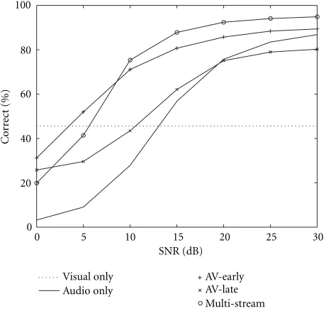
Figure 14 summarizes the performance of various recog-nizers. As can be seen, while the visual-only recognizer re-mains unaffected by acoustic noise, as must be the case since the signals were the same, the performance of the audio-only recognizer drops dramatically at high noise levels. A real-life experiment with actual noise might show variations in the visual only performance due to the Lombard effect [64, 65], but this aspect was not investigated (the Lombard effect was examined for example in study [66]).
In the speaker-dependent speech recognition, the multi-stream model performs the best among the three AV models at high SNR. Compared with the early integration model, the multistream model better explains the relations between the audio and video channels in this SNR range by emphasizing the reliability of the acoustic channel more. However at low SNR, the weighting factors ofγA=0.7 andγV =0.3 are not appropriate any more, since the visual source of information becomes relatively more reliable.
Apart from the exception at high SNR for the late inte-gration, all integrated models demonstrate improved recog-nition accuracy over audio-only results. However, the per-formance of the integrated systems drops below the perfor-mance of the visual-only system at very low SNRs, because the bad acoustic recognizer pulls down the total result. It is observed that the visual contribution is most distinct at low SNR. When the performance of the acoustic recognizer
30
Figure 14: Performance comparison for various audio-visual speaker-dependent speech recognition systems under mismatched conditions. Recognition in speaker-dependent mode.
improves with increasing SNRs, the benefit of the addition of the visual component becomes less visible because there is less room for improvement. In total, when the best AV inte-gration model is used, we obtain a performance gain of 27.97 percentage points at 0 dB and 8.05 percentage points at 30 dB over audio-only.
The CMU database [33] has been studied by several other groups [34, 67] for audio-visual speech recognition. How-ever, only partial vocabulary and test subjects were used. To our knowledge, the results presented here are the first ones that evaluated the entire database.
5. SPEAKER VERIFICATION
The speaker verification task corresponds to an open test set scenario where persons who are unknown to the system might claim access. The world population is divided into two categories—a client who is known to the system, and imposters who falsely claim to have the identity of a client. Speaker verification is to validate a claimed identity: either to accept or reject an identity claim. Two types of error are pos-sible: false acceptance of an imposter (FA), and false rejection of a client (FR).
For the speaker verification task, we use the polynomial-based approach [68]. Polynomial-polynomial-based classification re-quires low computation while maintaining high accuracy. Because of the Weierstrass approximation theorem, poly-nomials are universal approximators for the Bayes classifier [69].
The classifier consists of several parts as shown in Figure 15. The extracted feature vectors o1, . . . ,oN are
in-troduced to the classifier. For each feature vector oi, a
Accept
Figure15: Structure of a polynomial classifier.
function d(o,w) = wTp(o), where p(o) is the polynomial
basis vector constructed from the input vector o,p(o) =
[1 o1 o2 o21 o1o2 o22]T for a two-dimensional feature
vec-toro = [o1 o2]T and for polynomial order two, andw is
the class model. The polynomial discriminant function ap-proximates the a posteriori probability of the client/impostor identity given the observation [69]. In [70, 71], a statistical interpretation of scoring was developed. The final score is computed by averaging over all feature vectors
Score= 1
The accept/reject decision is performed by comparing the output score to a threshold. If Score < T, then reject the claim, otherwise, accept the claim.
The verification system requires discriminative training in order to maximize its accuracy. For a speaker’s features, an output value of 1 is desired. For impostors’ features, an output of 0 is desired. The optimization problem can be for-mulated using a mean-squared error criterion
wspk=arg min
incorporate the weighting factors in (16) is to balance the number of vectors in the two classes, since normally there is a large amount of data for impostors and only a few values for the user. This equalization prevents overtraining on the impostor data set.
When expressed in matrix form, (16) can be rewritten as
wspk=arg min
w DMw−Du2, (17)
where Dis a diagonal matrix,u is the vector consisting of
Nspkones followed byNimpzeros, and
M=
It can be shown that (17) can be solved [72] by using
are of fixed size andRimpcan be precomputed and stored in
advance.
We perform the speaker verification test on the XM2VTS database [35]. This database includes four recordings of 295 subjects taken at one month intervals. (However we were able to use only 261 of the 295 speakers because of corrupted au-dio or video sequences [73].) Each sequence is approximately 5 seconds long and contains the subject speaking the sen-tence “Joe took father’s green shoe bench out.” The database covers a large population variation from various ethnic ori-gins and with various appearances. The same person might attend the four sessions with a different appearance, in-cluding hairstyles, with/without glasses, with/without beard, with/without lipstick. A snapshot of one person attending four sessions is shown in Figure 16.
To evaluate the performance of the person authentication systems on the XM2VTS database, we adopt the protocol de-fined in [74]. We chose configuration II due to the audio-visual data we are using. For the data partition defined in the protocol, each subject appears only in one set. This ensures realistic evaluation of the imposter claims whose identity is unknown to the system.
Figure16: Snapshot of the XM2VTS database [35].
25 20
15 10
5 0
SNR (dB) 0
0.05 0.1 0.15 0.2 0.25 0.3 0.35 0.4 0.45 0.5
Er
ro
r
rat
e
Audio FRR Audio FAR Visual FRR
Visual FAR Fused FRR Fused FAR
Figure 17: Performance of audio-visual speaker verification in noisy conditions. Speaker verification FRR and FAR at EER in vary-ing noise conditions
imposter, and the FRR is the percentage of times access is de-nied to a valid claimant. The pooled equal error rate (EER) threshold at which FAR=FRR is determined from the eval-uation set and used against the test population to determine the system performance. Both FAR and FRR are reported for this operating point. The test results for a visual-only speaker verification system are shown in Table 2.
In our experiment, polynomial orders two and three are used. The visual features included are the eight parameters derived in Section 3. Extra features are the corresponding delta features and the normalized time indexi/M, whereiis the current frame index, andMis the total number of frames. Since the score in a polynomial-based classifier (15) is an av-erage of all feature vectors, the time index carries temporal information within the spoken sentence. As can be seen, by incorporating extra features, a lower error rate is achieved. At the same time, increasing the polynomial order also con-tributes to improved verification results.
To our knowledge, there were no other published results on using visual speech features for the speaker verification experiments based on the XM2VTS database
Table 2: Performance for the speaker verification tasks using database [35].
Features Poly. order FRR% FAR%
All (8) 2 8.8 9.7
All +∆(16) 2 6.1 9.3
All (8) 3 5.0 9.0
All +∆(16) 3 4.4 8.2 All + time (9) 2 8.3 9.2 All + time (9) 3 4.8 8.5
(Studies [13, 75] performed speaker verification experiments on a smaller set of the M2VTS database). However, the XM2VTS database has been extensively used by the face recognition community. A face verification contest was orga-nized at theInternational Conference on Pattern Recognition, 2000 to promote a competition for the best face verification algorithm. The tests were carried out using the static image shots of the XM2VTS database. All research groups partic-ipated in the contest used the same database and the same protocol for training and evaluation. A total of fourteen face verification methods were tested and compared [76]. For the same configuration as carried out in our speaker verification experiments, the published results of FAR/FRR range from 1.2/1.0 to 13.0/12.3. This suggests that our speaker verifica-tion approach that uses the lip modality is comparable to the state-of-the-art face-based personal authentication methods. In the audio modality, each feature vector is composed of 12 cepstral coefficients and one normalized time index [68]. A third-order polynomial classifier is used. To fuse the two modalities, we use a late integration strategy. We combine the classifier outputs from the audio and visual modalities by averaging the class scores,s=αsA+ (1−α)sV, wheresA,V are computed from (15) for the audio and visual channels. For the following experiments, the audio and visual modalities are weighted equally (i.e.,α=0.5).
be seen, the contribution of the visual modality is most dis-tinct at low SNR. We observe an error rate drop of 36 per-centage points for FRR and 32 perper-centage points for FAR at 0 dB over audio-only when visual modality is incorporated. As illustrated in the figure, the audio-visual fusion is shown to outperform both modalities at high signal-to-noise ratios. However, error rates over the low range of signal-to-noise ra-tios (SNR) are worse than the visual-only results and it indi-cates that a dynamic fusion strategy, for example, adjusting the weighting of the modalities as SNR degrades, may im-prove the overall system performance.
6. SUMMARY
In this paper, we described a method of automatic lip feature extraction and its applications to speech and speaker recog-nition. Our algorithm first reliably locates the mouth re-gion by using hue/saturation and motion information from a color video sequence of a speaker’s frontal view. The algo-rithm subsequently segments the lip from its surroundings by making use of both color and edge information, combined within a Markov random field framework. The lip key points that define the lip position are detected and the relevant vi-sual speech parameters are derived and form the input to the recognition engine. We then demonstrated two applications by exploring these visual parameters. Experiments for auto-matic speech recognition involve discrimination of a set of 78 isolated words spoken by ten subjects [33]. It was found that by enabling extraction of an expanded set of visual speech features including the lip inner contour and the visibility of the tongue and teeth, the proposed visual front end achieves an increased accuracy when compared with previous stud-ies that use only lip outer contour features. Three popular audio-visual integration schemes were considered and the visual information is shown to improve recognition perfor-mance over a variety of acoustic noise levels. In the speaker verification task, we employed a polynomial based approach. The speaker verification experiments on the database with 261 speakers achieve an FRR of 4.4% and an FAR of 8.2% with polynomial order 3, and suggest that visual information is highly effective in reducing both false acceptance and false rejection rates in such tasks.
ACKNOWLEDGMENTS
The research on which this paper is based acknowledges the use of the extended multimodal face database and associated documents [35, 36]. We would also like to acknowledge the use of audio-visual data [33, 34] from the Advanced Multi-media Processing Lab at the Carnegie Mellon University.
REFERENCES
[1] T. Sullivan and R. Stern, “Multi-microphone correlation-based processing for robust speech recognition,” inProc. IEEE Int. Conf. Acoustics, Speech, Signal Processing, pp. 91–94, Min-neapolis, Minn, USA, April 1993.
[2] R. M. Stern, A. Acero, F.-H. Liu, and Y. Ohshima, “Signal pro-cessing for robust speech recognition,” inAutomatic Speech
and Speaker Recognition: Advanced Topics, C.-H. Lee, F. K. Soong, and K. K. Paliwal, Eds., pp. 357–384, Kluwer Academic Publishers, Boston, Mass, USA, 1996.
[3] O. Ghitza, “Auditory nerve representation as a front-end for speech recognition in a noisy environment,”Computer Speech and Language, vol. 1, no. 2, pp. 109–130, 1986.
[4] B.-H. Juang, “Speech recognition in adverse environments,” Computer Speech and Language, vol. 5, no. 3, pp. 275–294, 1991.
[5] W. H. Sumby and I. Pollack, “Visual contribution to speech intelligibility in noise,” Journal of the Acoustical Society of America, vol. 26, no. 2, pp. 212–215, 1954.
[6] N. P. Erber, “Interaction of audition and vision in the recog-nition of oral speech stimuli,” Journal of Speech and Hearing Research, vol. 12, pp. 423–425, 1969.
[7] E. D. Petajan, Automatic lipreading to enhance speech recogni-tion, Ph.D. thesis, University of Illinois, Urbana-Champaign, Ill, USA, 1984.
[8] D. G. Stork and M. E. Hennecke, Eds., Speechreading by Hu-mans and Machines, vol. 150 ofNATO ASI Series F: Computer and Systems Sciences, Springer-Verlag, Berlin, Germany, 1996. [9] C. Neti, G. Potamianos, J. Luettin, et al., “Audio-visual speech recognition,” Tech. Rep., CLSP/Johns Hopkins University, Baltimore, Md, USA, 2000.
[10] R. Chellappa, C. L. Wilson, and S. Sirohey, “Human and ma-chine recognition of faces: A survey,”Proceedings of the IEEE, vol. 83, no. 5, pp. 705–740, 1995.
[11] P. S. Penev and J. J. Atick, “Local feature analysis: A general statistical theory for object representation,”Network: Compu-tation in Neural Systems, vol. 7, no. 3, pp. 477–500, 1996. [12] J. Luettin,Visual speech and speaker recognition, Ph.D. thesis,
University of Sheffield, Sheffield, UK, 1997.
[13] T. J. Wark and S. Sridharan, “A syntactic approach to au-tomatic lip feature extraction for speaker identification,” in Proc. IEEE Int. Conf. Acoustics, Speech, Signal Processing, vol. 6, pp. 3693–3696, Seattle, Wash, USA, May 1998.
[14] B. P. Yuhas, M. H. Goldstein, and T. J. Sejnowski, “Integration of acoustic and visual speech signals using neural networks,” IEEE Communications Magazine, vol. 27, pp. 65–71, Novem-ber 1989.
[15] C. Bregler, H. Hild, S. Manke, and A. Waibel, “Improved connected letter recognition by lipreading,” in Proc. IEEE Int. Conf. Acoustics, Speech, Signal Processing, pp. 557–560, Minneapolis, Minn, USA, 1993.
[16] C. Bregler and Y. Konig, “Eigenlips for robust speech recog-nition,” inProc. IEEE Int. Conf. Acoustics, Speech, Signal Pro-cessing, vol. 2, pp. 669–672, Adelaide, Australia, 1994. [17] P. L. Silsbee and A. C. Bovik, “Computer lipreading for
improved accuracy in automatic speech recognition,” IEEE Trans. Speech, and Audio Processing, vol. 4, no. 5, pp. 337–351, 1996.
[18] G. Potamianos, J. Luettin, and C. Neti, “Hierarchical dis-criminant features for audio-visual LVCSR,” inProc. IEEE Int. Conf. Acoustics, Speech, Signal Processing, pp. 165–168, Salt Lake City, Utah, USA, May 2001.
[19] K. Mase and A. Pentland, “Automatic lipreading by optical flow analysis,”Systems and Computers in Japan, vol. 22, no. 6, pp. 67–75, 1991.
[20] A. J. Goldschen, O. N. Garcia, and E. Petajan, “Continuous optical automatic speech recognition by lipreading,” inIEEE Proc. the 28th Asilomar Conference on Signals, Systems and Computers, pp. 572–577, Pacific Grove, Calif, USA, October– November 1994.
[22] M. Kass, A. Witkin, and D. Terzopoulos, “Snakes: Active con-tour models,”International Journal of Computer Vision, vol. 1, no. 4, pp. 321–331, 1988.
[23] J. Luettin, N. A. Thacker, and S. W. Beet, “Active shape mod-els for visual speech feature extraction,” inSpeechreading by Humans and Machines, D. G. Stork and M. E. Hennecke, Eds., vol. 150 ofNATO ASI Series F: Computer and Systems Sciences, pp. 383–390, Springer-Verlag, Berlin, 1996.
[24] M. U. Ramos Sanchez, J. Matas, and J. Kittler, “Statisti-cal chromaticity models for lip tracking with B-splines,” in Proc. the 1st Int. Conf. on Audio- and Video-Based Biometric Person Authentication, Lectures Notes in Computer Science, pp. 69–76, Springer-Verlag, Crans-Montana, Switzerland, 1997.
[25] M. Vogt, “Interpreted multi-state lip models for audio-visual speech recognition,” inProc. of the ESCA Workshop on Audio-Visual Speech Processing, Cognitive and Computational Ap-proaches, pp. 125–128, Rhodes, Greece, September 1997. [26] G. I. Chiou and J. Hwang, “Lipreading from color video,”
IEEE Trans. Image Processing, vol. 6, no. 8, pp. 1192–1195, 1997.
[27] M. Chan, “Automatic lip model extraction for constrained contour-based tracking,” inProc. IEEE International Confer-ence on Image Processing, vol. 2, pp. 848–851, Kobe, Japan, Oc-tober 1999.
[28] A. A. Montgomery and P. L. Jackson, “Physical characteristics of the lips underlying vowel lipreading performance,”Journal of the Acoustical Society of America, vol. 73, no. 6, pp. 2134– 2144, 1983.
[29] A. Q. Summerfield, “Lipreading and audio-visual speech per-ception,”Philosophical Transactions of the Royal Society of Lon-don, Series B, vol. 335, no. 1273, pp. 71–78, 1992.
[30] A. Q. Summerfield, A. MacLeod, M. McGrath, and M. Brooke, “Lips, teeth and the benefits of lipreading,” in Handbook of Research on Face Processing, A. W. Young and H. D. Ellis, Eds., pp. 223–233, Elsevier Science Publishers, Amsterdam, North Holland, 1989.
[31] M. McGrath, An examination of cues for visual and audio-visual speech perception using natural and computer-generated face, Ph.D. thesis, University of Nottingham, Nottingham, UK, 1985.
[32] D. Rosenblum and M. Salda˜na, “An audiovisual test of kine-matic primitives for visual speech perception,” Journal of Experimental Psychology: Human Perception and Performance, vol. 22, no. 2, pp. 318–331, 1996.
[33] http://amp.ece.cmu.edu/projects/audiovisualspeechprocess-ing .
[34] T. Chen, “Audiovisual speech processing: lip reading and lip synchronization,” IEEE Signal Processing Magazine, vol. 18, no. 1, pp. 9–21, 2001.
[35] http://www.ee.surrey.ac.uk/Research/vssp/xm2vtsdb. [36] K. Messer, J. Matas, J. Kittler, J. Luettin, and G. Maitre,
“XM2VTSDB: The extended M2VTS database,” inProc. 2nd Int. Conf. on Audio- and Video-Based Biometric Personal Veri-fication, pp. 72–77, Washington, DC, USA, March 1999. [37] C. Garcia and G. Tziritas, “Face detection using quantized
skin color regions merging and wavelet packet analysis,”IEEE Trans. Multimedia, vol. 1, no. 3, pp. 264–277, 1999.
[38] J. Yang, R. Stiefelhagen, U. Meier, and A. Waibel, “A real-time face tracker,” inProc. 3rd IEEE Workshop on Application of Computer Vision, pp. 142–147, Sarasota, Fla, USA, 1996. [39] K. Jack, Video Demystified: A Handbook for the Digital
Engi-neer, LLH Technology Publishing, Eagle Rock, Va, USA, 1996. [40] J. R. Kender, “Instabilities in color transformations,” IEEE
Computer Society, pp. 266–274, June 1977.
[41] N. Otsu, “A threshold selection method from gray level his-tograms,” IEEE Trans. Systems, Man, and Cybernetics, vol. 9, no. 1, pp. 62–66, 1979.
[42] M. J. Jones and J. M. Rehg, “Statistical color models with ap-plication to skin detection,”International Journal of Computer Vision, vol. 46, no. 1, pp. 81–96, 2002.
[43] A. W. Senior, “Face and feature finding for a face recogni-tion system,” inProc. 2nd International Conference on Audio-and Video-Based Biometric Person Authentication, pp. 154– 159, Washington, DC, USA, 1999.
[44] A. Hurlbert and T. Poggio, “Synthesizing a color algorithm from examples,”Science, vol. 239, pp. 482–485, January 1988. [45] S. Geman and D. Geman, “Stochastic relaxation, Gibbs dis-tribution, and the Bayesian restoration of images,” IEEE Trans. on Pattern Analysis and Machine Intelligence, vol. 6, no. 6, pp. 721–741, 1984.
[46] C. F. Borges, “On the estimation of Markov random field pa-rameters,”IEEE Trans. on Pattern Analysis and Machine Intel-ligence, vol. 21, no. 3, pp. 216–224, 1999.
[47] S. Geman and C. Graffigne, “Markov random field im-age models and their applications to computer vision,” in Proc. Int. Congress of Mathematicians, pp. 1496–1517, Berke-ley, Calif, USA, 1986.
[48] P. B. Chou and C. M. Brown, “The theory and practice of Bayesian image labeling,” International Journal of Computer Vision, vol. 4, no. 3, pp. 185–210, 1990.
[49] J. Marroquin, S. Mitter, and T. Poggio, “Probabilistic solution of ill-posed problems in computational vision,” inProc. Image Understanding Workshop, pp. 293–309, San Diego, Calif, USA, 1985.
[50] J. Marroquin, S. Mitter, and T. Poggio, “Probabilistic solu-tion of ill-posed problems in computasolu-tional vision,” Journal of American Statistical Association, vol. 82, no. 397, pp. 76–89, 1987.
[51] D. Geiger and F. Girosi, “Parallel and deterministic algorithms from MRFs: Surface reconstruction,” IEEE Trans. on Pattern Analysis and Machine Intelligence, vol. 13, no. 5, pp. 401–412, 1991.
[52] J. Besag, “On the statistical analysis of dirty pictures,”Journal of the Royal Statistical Society B, vol. 48, no. 3, pp. 259–302, 1986.
[53] P. Chou, C. Brown, and R. Raman, “A confidence-based ap-proach to the labeling problem,” inProc. IEEE Workshop on Computer Vision, pp. 51–56, Miami Beach, Fla, USA, 1987. [54] X. Zhang, R. M. Mersereau, M. Clements, and C. C. Broun,
“Visual speech feature extraction for improved speech recog-nition,” inProc. IEEE Int. Conf. Acoustics, Speech, Signal Pro-cessing, pp. 1993–1996, Orlando, Fla, USA, May 2002. [55] L. R. Rabiner and B. H. Juang,Fundamentals of Speech
Recog-nition, Prentice-Hall, Englewood Cliffs, NJ, USA, 1993. [56] L. E. Baum, T. Petrie, G. Soules, and N. Weiss, “A
maximiza-tion technique occurring in the statistical analysis of proba-bilistic functions of Markov chains,” Annals of Mathematical Statistics, vol. 41, no. 1, pp. 164–171, 1970.
[57] S. Young, D. Kershaw, J. Odell, D. Ollason, V. Valtchev, and P. Woodland, The HTK Book, Entropic, Cambridge, UK, 1999.
[58] A. Adjoudani and C. Benoit, “On the integration of au-ditory and visual parameters in an HMM-based ASR,” in Speechreading by Humans and Machines, D. G. Stork and M. E. Hennecke, Eds., vol. 150 ofNATO ASI Series F: Computer and Systems Sciences, pp. 461–471, Springer-Verlag, Berlin, 1996. [59] M. T. Chan, Y. Zhang, and T. S. Huang, “Real-time lip tracking
Sig-nal Processing, pp. 65–70, Los Angeles, Calif, USA, December 1998.
[60] R. R. Rao,Audio-visual interaction in multimedia, Ph.D. the-sis, Georgia Institute of Technology, Atlanta, Ga, USA, 1998. [61] S. Dupont and J. Luettin, “Audio-visual speech modelling for
continuous speech recognition,”IEEE Trans. Multimedia, vol. 2, no. 3, pp. 141–151, 2000.
[62] J. Luettin, G. Potamianos, and C. Neti, “Asynchronous stream modeling for large vocabulary audio-visual speech recogni-tion,” inProc. IEEE Int. Conf. Acoustics, Speech, Signal Process-ing, pp. 169–172, Salt Lake City, Utah, USA, May 2001. [63] J. R. Movellan and G. Chadderdon, “Channel
separabil-ity in the audio-visual integration of speech: A Bayesian ap-proach,” inSpeechreading by Humans and Machines, D. G. Stork and M. E. Hennecke, Eds., vol. 150 ofNATO ASI Se-ries F: Computer and Systems Sciences, pp. 473–487, Springer-Verlag, Berlin, 1996.
[64] E. Lombard, “Le signe de l’el´evation de la voix,” Ann. Mal-adiers Oreille, Larynx, Nez, Pharynx, vol. 37, pp. 101–119, 1911.
[65] H. L. Lane and B. Tranel, “The Lombard sign and the role on hearing in speech,” Journal of Speech and Hearing Research, vol. 14, no. 4, pp. 677–709, 1971.
[66] F. J. Huang and T. Chen, “Consideration of Lombard effect for speechreading,” inProc. Workshop Multimedia Signal Pro-cessing, pp. 613–618, Cannes, France, October 2001.
[67] A. V. Nefian, L. Liang, X. Pi, X. Liu, C. Mao, and K. Murphy, “A coupled HMM for audio-visual speech recognition,” in Proc. IEEE Int. Conf. Acoustics, Speech, Signal Processing, pp. 2013–2016, Orlando, Fla, USA, May 2002.
[68] C. C. Broun and X. Zhang, “Multimodal fusion of polyno-mial classifiers for automatic person recognition,” inSPIE 15th AeroSense Symposium, pp. 166–174, Orlando, Fla, USA, April 2001.
[69] J. Schuermann, Pattern Classification, a Unified View of Sta-tistical and Neural Approaches, John Wiley & Sons, New York, USA, 1996.
[70] W. M. Campbell and C. C. Broun, “Using polynomial net-works for speech recognition,” inNeural Networks for Signal Processing X, Proceedings of the 2000 IEEE Workshop, pp. 795– 803, Sydney, Australia, 2000.
[71] W. M. Campbell, K. T. Assaleh, and C. C. Broun, “Speaker recognition with polynomial classifiers,”IEEE Transactions on Speech and Audio Processing, vol. 10, no. 4, pp. 205–212, 2002. [72] G. H. Golub and C. F. Van Loan,Matrix Computations, John Hopkins University Press, Baltimore, Md, USA, 2nd edition, 1989.
[73] http://users.ece.gatech.edu/xzhang/note on defect seq in xm 2vts.txt.
[74] J. Luettin and G. Maitre, “Evaluation protocol for the XM2VTS database,” IDIAP-COM 98-05, IDIAP, October 1998.
[75] P. Jourlin, J. Luettin, D. Genoud, and H. Wassner, “Acoustic-labial speaker verification,”Pattern Recognition Letters, vol. 18, no. 9, pp. 853–858, 1997.
[76] J. Matas, M. Hamouz, K. Jonsson, et al., “Comparison of face verification results on the XM2VTS database,” inProc. the 15th International Conference on Pattern Recognition, A. San-feliu, J. J. Villanueva, M. Vanrell, R. Alqueraz, J. Crowley, and Y. Shirai, Eds., vol. 4, pp. 858–863, Los Alamitos, Calif, USA, September 2000.
Xiaozheng Zhangreceived the Diploma in electrical engineering in 1997 from the Uni-versity of Erlangen-Nuremberg, Germany. In the same year, she joined the Telecom-munications Institute at the same univer-sity, where she worked on motion com-pensation related video compression tech-niques. Starting from winter 1998, she con-tinued her education at the Georgia Insti-tute of Technology, Atlanta, GA, where she
conducted research on joint audio-visual speech processing. She re-ceived the Ph.D. degree in electrical and computer engineering in May 2002. She is the recipient of the 2002 Outstanding Research Award from the Center of Signal and Image Processing, Georgia Institute of Technology. Her research interests are in the areas of computer vision, image analysis, statistical modeling, data fusion, and multimodal interaction.
Charles C. Brounreceived his B.S. degree in 1990, and the M.S. degree in 1995, both in electrical engineering from the Geor-gia Institute of Technology. He specialized in digital signal processing, communica-tions, and optics. From 1996 to 1998, he conducted research in speech and speaker recognition at Motorola SSG in the Speech and Signal Processing Lab located in Scotts-dale, Arizona. There he worked both the
speaker verification product CipherVOX, and the System Voice Control component of the U.S. Army’s Force XXI/Land War-rior program. In 1999 he joined the newly formed Motorola Labs—Human Interface Lab in Tempe, Arizona, where he ex-panded his work tomultimodalspeech and speaker recognition. Currently, he is the project manager for several realization ef-forts within the Human Interface Lab—Intelligent Systems Lab. The most significant is the Driver Advocate, a platform sup-porting research in driver distraction mitigation and workload management.
Russell M. Mersereaureceived his S.B. and S.M. degrees in 1969 and the Sc.D. degree in 1973 from the Massachusetts Institute of Technology. He joined the School of Electri-cal and Computer Engineering at the Geor-gia Institute of Technology in 1975. His cur-rent research interests are in the develop-ment of algorithms for the enhancedevelop-ment, modeling, and coding of computerized im-ages, and computer vision. He is the
Mark A. Clementsreceived the S.B. degree in 1976, the S.M. degree in 1978, the Elec-trical Engineering degree in 1979, and the Sc.D. degree in 1982, all in electrical engi-neering and computer science from MIT. During his graduate work, he was sup-ported by a National Institutes of Health fel-lowship for research in hearing prostheses, and corporate sponsorship for the develop-ment of real-time automatic speech

![Table 1: Recognition rates for visual speech recognition using database [33]. The numbers represent the percentage of correct recognition.](https://thumb-us.123doks.com/thumbv2/123dok_us/889006.1106892/13.612.112.489.94.327/recognition-recognition-database-numbers-represent-percentage-correct-recognition.webp)