Volume 2010, Article ID 203178,7pages doi:10.1155/2010/203178
Research Article
A Linear Mixed-Effects Model of Wireless Spectrum Occupancy
Srikanth Pagadarai and Alexander M. Wyglinski
Department of Electrical and Computer Engineering, Worcester Polytechnic Institute, Worcester, MA 01609, USA
Correspondence should be addressed to Alexander M. Wyglinski,[email protected]
Received 6 January 2010; Revised 4 July 2010; Accepted 24 August 2010
Academic Editor: R. C. De Lamare
Copyright © 2010 S. Pagadarai and A. M. Wyglinski. This is an open access article distributed under the Creative Commons Attribution License, which permits unrestricted use, distribution, and reproduction in any medium, provided the original work is properly cited.
We provide regression analysis-based statistical models to explain the usage of wireless spectrum across four mid-size US cities in four frequency bands. Specifically, the variations in spectrum occupancy across space, time, and frequency are investigated and compared between different sites within the city as well as with other cities. By applying the mixed-effects models, several conclusions are drawn that give the occupancy percentage and the ON time duration of the licensed signal transmission as a function of several predictor variables.
1. Introduction
Spectrum measurement studies conducted by wireless com-munications researchers have shown that the utilization of licensed wireless spectrum is relatively low [1]. This is a result of the fact that frequency bands are exclusively licensed to specific services and entities on a
command-and-controlbasis by regulatory agencies, for example, U.S. Federal
Communications Commission (FCC), Industry Canada, and U.K. Office of Communications (OfCom). Although such a scheme is effective in protecting the rights of the incumbent license holders, a completely new strategy of spectrum allocation is needed in order to accommodate the increasing need for efficiently utilizing the wireless spectrum. This new strategy, calleddynamic spectrum access(DSA), can be enabled by highly agile wireless platforms called cognitive
radios[2]. Recently, as a significant step in this direction, the
FCC has adopted the initial rules for the use of unlicensed devices in TV bands [3]. Consequently, there is a need to accurately assess and characterize wireless spectrum in order to facilitate the transition to this new spectrum allocation strategy.
Some of the earlier works aimeing at quantifying the spectrum usage within the context of DSA-oriented cogni-tive radio using actual real-time measurements have been reported in [1,4]. A comprehensive summary of spectrum occupancy for New York City and several locations in
Virginia were reported in [1]. Reference [4] presents similar results for locations in the state of Georgia. In particular, spectrum occupancy variations as a function of varying thresholds and across the different angles of arrival at the receiver were presented. In [5], a more thorough math-ematical analysis based on continuous-time semi-Markov models is provided using spectrum measurement data of WLAN channels. More recently, closed-form probability distributions are presented for several fixed bandwidth signalling channels in [6] using the datasets presented in [1] whereas in [7], a comparison of the spectrum occupancy characteristics in four mid-size US cities is provided.
Spectrum measurement-based studies similar to those described above have also been conducted outside of the United States. In [8], spectrum occupancy for several bands in the frequency range from 806 MHz to 2750 MHz in urban Auckland, New Zealand is provided. In [9], four spectrum sensing methods have been proposed, and their performance is compared for UMTS uplink and GSM 1800 uplink bands. In [10], a methodology has been developed to identify TV whitespace frequencies in the UK, using digital TV coverage maps in conjunction with a database containing their locations.
Table1: List of spectrum measurement locations.
Location City
ROCHESTER, NY BUFFALO, NY PITTSBURGH, PA WORCESTER, MA
19th & 20th June 2008 21st & 22nd June 2008 23rd & 24th June 2008 17th, 26th, & 27th July 2008 SITE 1 S. Plymouth & E. Huron St. & 16th St Bridge & SE of Boynton Hall
Exchange Blvd Washington St. N of 1711 Penn. Av. WPI
SITE 2 Jay St. & Swan St. & Sheraton St. & Vernon St. &
Verona St. E. Michigan Av. Fort Pitt Bridge Dorchester St.
SITE 3 Prince St. & Pearl St. & Riverfront Park next to Bell Hill Park
Univ. Av. Church St. Birmingham bridge (offBelmont St.)
SITE 4 Mortimer St. & W. Genesee St. & Craig St. & Major Taylor Blvd. &
N. Clinton St. Seventh St. N. 5th Av. Thomas St.
SITE 5 Pearl St. & Oak St. & Grandview St. & Gateway Park (Parking lot)
Averill Av. Clinton St. Ulysses St. WPI
independently conducted measurement campaigns, there still exists a definite need to obtain a deeper understanding of this natural resource. By gaining insights into wireless spectrum occupancy characteristics, appropriate technical and legislative actions can be taken in order to support con-tinued growth in the wireless sector. In this paper, we present a statistical analysis for the wireless spectrum occupancy across the spatial, temporal, and frequency dimensions using measurements collected in four mid-size US cities, namely, Rochester, NY; Buffalo, NY; Pittsburgh, PA; Worcester, MA. Although we have collected these measurements across several bands within the 88 MHz–3 GHz frequency range, results pertaining to only certain bands are presented for the purpose of brevity.
The rest of this paper is organized as follows. InSection 2, the measurement setup consisting of the hardware and software tools used to collect the data is described. Then, a description of the statistical results extracted from the measured data is presented inSection 3. A brief discussion of the linear mixed-effects model followed by its application to the collected measurement data is provided in Sections4
and5. Finally, we conclude the paper by highlighting the key conclusions inSection 4.
2. Spectrum Measurement Setup
In our measurement campaign, we used two antennas for scanning the low- and the high-frequency ranges. For the low-frequency range, from 88 MHz to 1240 MHz, we used a Diamond D-220 mini-Discone antenna with an operating frequency range of 100–1600 MHz. For the high-frequency range, from 1850 MHz to 2686 MHz, we used an Advanced Technical Materials (ATM) 07-18-440-NF horn antenna with an operating frequency range of 0.7–18 GHz and an aperture of 60◦. This helped us in observing the variation in spectrum usage across different angles of arrival. During our operation, one of these antennas is wired to an Agilent CSA seriesN1996Aspectrum analyzer with frequency range
ranging from 100 kHz to 3 GHz and consisting of a low-noise amplifier (LNA). We use an in-house software tool called SQUIRREL (Spectrum Query Utility Interface for Real-time Radio Electromagnetics) to communicate remotely with the spectrum analyzer via commands issued through a simple graphical user interface on a laptop. The GUI accepts details such as the center frequency, the span around the center frequency, and the resolution bandwidth. SQUIRREL communicates with the spectrum analyzer using TCL (Tool Command Language) over TCP/IP. After the sweep action is performed by the spectrum analyzer, the data points are returned to the GUI in a comma-spaced value format. In its current format, the GUI and the server are written in JAVA and can be deployed on a variety of operating systems and computers.
0
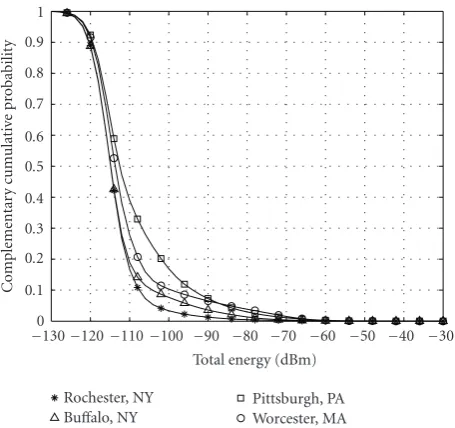
Figure 1: Cumulative distribution functions showing spectrum occupancy for the four cities surveyed.
3. Spectrum Occupancy Characteristics
Figure 1 shows the trend in the occupancy irrespective of the cities, sites, time, and frequency. Although it serves the purpose of summarizing the measured results, a great deal of details remain hidden in the data with respect to both the occupancy characteristics over time, frequency, and space, and their dependance on other influencing factors. One way of analyzing the occupancy results is presented in [7] where we have provided occupancy values in percentages across different channels, along different angles of arrival and over several time sweeps as observed during the measurement duration. Another way of performing the analysis is from the point of associating the measured data with certainpredictor
variables in a linear mixed-effects model as we will explain
below.
Due to the differences in the signal modulation involved as well as the differences in the bandwidths utilized by each channel, energy spectral densities corresponding to signals transmitted for different wireless services can be expected to be different. Thus, the four different wireless services analyzed, namely, paging, TV, WCS, and PCS correspond to four different predictor variables. Similarly, the four US cities are also predictor variables. Assuming that the spectrum usage is dependant on two other factors, namely, the time of the day and day of the week, they are incorporated as well. Due to the fact that our data corresponds to only four mid-size US cities, we do not claim that our model is a representative of all the mid-size US cities. This is the reason why although our model is not as general as we would like it to be, due to practical constraints involved, we, nevertheless, believe that it is indicative of the general trends in spectrum occupancy characteristics that can be expected in any typical US city. Moreover, we considered the population densities associated with the measurement sites as our random-effects
term to reflect this fact. In the following sections, we provide more details regarding the occupancy values by grouping the appropriate collected data points as functions of several predictor variables. We now briefly explain the algorithm used to determine the presence/absence of the licensed user signal.
In order to show a comparison of the spectrum usage as a function of the variables mentioned above, an optimum threshold is computed using Otsu’s gray-level thresholding algorithm [11] for each of the datasets. Otsu’s optimum threshold provides a maximum separation between the two classes of data, namely, the signal and the noise (There are alternative approaches for computing the threshold, some of which are explained in [4]). Our primary motivation to use Otsu’s thresholding algorithm is influenced by the nature of the data collected. Our measured data is in fact samples of energy spectral density (ESD) across a band of concentration and not time samples. We cannot apply traditional signal detection-based techniques due to total absence of phase information. Therefore, we detect the presence of the signal in the data purely from the point of view of separating data into two distinct distributions. The optimal threshold calculated using Otsu’s algorithm is known to maximize the variance between the two classes of data, namely, the signal and the noise classes. Therefore, we employ this algorithm in our analysis.
In order to apply Otsu’s algorithm, a matrix M(tj,fi)
is formed from the collected data points where the rowtj
contains data points over all the frequency locations in the band of interest during one particular time instant, and the column fi represents the data points observed in that
frequency bin over all time sweeps during the measurement process. The next step is to transform the contents of this matrix into gray-scale values by applying the procedure given by
Applying Otsu’s algorithm to the matrix,I(tj,fi), gives the
4. An Overview of the Linear
Mixed-Effects Model
The normal linear model given by the equation:
yi=β1x1i+β2x2i+· · ·+βpxpi+εi, (2)
explains the relationship between one or more independent variables, calledregressor variables, and a dependent variable, called theresponse variable. The parameters of the model are called the regression coefficients, specified asβ1, β2,. . .,βp,
and theerror variance, defined asσ2. The above model has
onerandom-effectterm, the error termεigiven by
εi∼N
0,σ2, (3)
which is assumed to be independent and identically dis-tributed (i.i.d.). Another important assumption is that the sample is drawn randomly from the population of interest. Usually, we set x1i = 1 while β1 is either a constant or an
intercept. Therefore, rewriting the model in matrix form yields
where we define the following variables:
(i) y=[y1,y2,. . .,yn]Tis the response vector;
(ii)Xis the model matrix;
(iii)β = [β1,β2,. . .,βn]T is the vector of regression
coefficients;
(iv)ε=[ε1,ε2,. . .,εn]Tis the vector of errors;
(v)Nn represents the n-variable multivariate normal
distribution.
Estimating the parameters of the above model is a well known linear least squares problem. The estimate of the regression coefficient vector is given by the expression:
β=XTX−1XTy. (5)
Several variants of the basic linear regression model of (2) are widely used in various areas of science. One such variant is themixed-effect model. These models include additional random-effect terms and are appropriate in representing clustered, and therefore, dependent data arising when data are collected over time on the same entities; that is, theserepeated measures dataare generated by observing a number of entities repeatedly under differing experimental conditions, where the entities are assumed to constitute a random sample from a population of interest. Longitudinal data constitute a common type of repeated measures data, where the observations are ordered by time or position in space. In general, longitudinal data can be defined as repeated measures data where the observations within entities could not have been randomly assigned to the levels of a “treatment” of interest (usually time or position in space); hence, serial correlation results.
Writing the linear mixed-effect model of the form shown in (2) yields
Alternately, but equivalently, the above model can be written in matrix form as
where we define the following variables:
(i) yiis theni×1 response variable for observations in
theith group;
(ii)Xiis theni×pmodel vector for the fixed effects for
observations in theith group;
(iii)βis thep×1 vector of fixed-effects coefficients for the ith group;
(iv)Ziis theni×qmodel matrix for the random effects
for observations in theith group;
(v)biis theq×1 vector of random-effects coefficients for
i×nicovariance matrix for the errors in
theith group.
From the above representation, defineX = [X1T,X2T,. . ., XMT]T,D =diag(D1,D2,. . .,DM) andZ=diag(Z1,Z2,. . ., ZM).When the variance componentsΛandDare known,
the standard estimators forβandbare the generalized linear estimatorβlin =(XTV−1X)−1
XTV−1ywhereV=Λ+ZDZT and the posterior mean, blin = DZTV−1(y −Xβ). The estimatesβlin andblin jointly maximize the function [12]:
glinβ,b|y= −1
Table2: Fixed effects.
Coefficient Std. Error DF t-value P-value
(Intercept) 13.28 0.244 473 54.354 <.0001
TV 5.82 0.317 473 18.36 <.0001
PCS 4.33 0.225 473 19.23 <.0001
WCS 4.08 0.202 473 20.11 <.0001
Roch 1.37 0.423 473 3.23 7e-4
Buff 4.98 0.273 473 18.21 <.0001
Pitt 3.67 0.356 473 10.29 <.0001
AN 0.5 0.159 473 3.15 9e-4
Weekend −1.12 0.116 473 −9.68 <.0001
Table3: Fixed effects.
Coefficient Std. Error DF t-value P-value
(Intercept) 2.33 0.12 473 19.44 <.0001
TV 2.21 0.132 473 16.73 <.0001
PCS 1.02 0.056 473 18.23 <.0001
WCS 1.24 0.24 473 5.16 <.0001
Roch 2.12 0.474 473 4.47 <.0001
Buff 3.26 0.778 473 4.19 <.0001
Pitt 2.74 0.769 473 3.56 2e-4
AN 2.03 0.76 473 2.67 <.0001
Weekend −1.87 0.227 473 −8.23 <.0001
5. Linear Mixed-Effects Model Applied to
Real-Time Wireless Spectrum Analysis
5.1. Regression Fit for Percentage Spectrum Occupancy. The
model for the performed analysis on the spectrum occupancy percentage using a linear mixed model is as follows:
Occ.Perci j=β0+β1TVi j+β2PCSi j+β3WCSi j
+β4rochi j+β5buffi j+β6pitti j+β7ANi j
+β8weekendi j+bi0+bi1PDi j+εi j.
(10)
As seen from the above model, we have selected three indica-tor variables (i.e., either 1 or 0) for the types of the wireless service (TV, PCS, WCS), three indicator variables for the cities (Rochester, Buffalo, Pittsburgh), one indicator variable for afternoon/before noon, and one indicator variable for weekend/weekday. The intercept represents the spectrum occupancy in the paging band for Worcester, Massachusetts. As mentioned previously, the response variable in the regression analysis that we considered is the percentage spectrum occupancy which is calculated after applying Otsu’s thresholding algorithm. Also, notice that the population density of the sites is chosen as the random-effects term which is specific to each of 20 groups (4 cities ×5 sites). Since, we collected 25 wireless spectrum sweeps in each of the 5 sites from each city, the population density is
chosen as the random effect that is different among the sites. Moreover, the population density is rounded off to the next highest multiple of 100. Thus, discrete values are considered, which helps in the interpretation of the obtained results. Fitting the linear mixed model gives the following results inTable 2. The parameters associated with the random effects are as follows: standard deviation of the intercept=2.14, standard deviation of the population density
= 0.12, and the correlation coefficient of the population density=0.007.
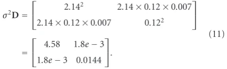
From the above random effects, the covariance matrix of the random effects [13] can be calculated as follows:
σ2D= ⎡
⎣ 2.142 2.14×0.12×0.007 2.14×0.12×0.007 0.122
⎤ ⎦
= ⎡
⎣ 4.58 1.8e−3 1.8e−3 0.0144
⎤ ⎦.
(11)
5.1.1. Interpretation of the Obtained Regression Fit. From
−3
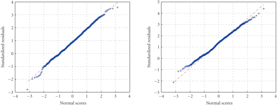
(a) Quantile-quantile plot for the fit shown in (10)
−3
(b) Quantile-quantile plot for the fit shown in (12)
Figure2: Quantile-quantile plots for the proposed linear mixed-effects models.
consideration, the type of the wireless service, and the time of the day remaining constant, the spectrum occupancy decreases by 1.12% on the weekends for aP-value of< .0001. Notice that we have obtained all of the above coefficients at very lowP-values indicating the statistical significance of each of the regressors. Also, the structure of the Dmatrix which is almost diagonal suggests that the assumed normality assumption on the random effects is valid. The plot of the standardized residuals shown in Figure 2(a) also supports this assumption on the residuals since approximately 95% of the residuals lie in the range [−1.96, +1.96]; that is, they follow a standard normal distribution very closely.
5.2. Regression Fit for ON Time Duration of the Licensed Signal
Transmissions. The model for the performed analysis on the
ON time duration of the licensed signal transmissions in the four bands considered is similar to that of the spectrum occupancy percentage. Thus, it follows that
ON.timei j=β0+β1TVi j+β2PCSi j+β3WCSi j
+β4rochi j+β5buffi j+β6pitti j+β7ANi j
+β8weekendi j+bi0+bi1PDi j+εi j.
(12)
In this case, the response variable in the regression analysis performed is the ON time duration which is calculated after applying Otsu’s thresholding algorithm. We calculated the amount of time during which the licensed signal transmission was consistently above the calculated threshold. The regressor variables are the same. Fitting the linear mixed model gives the following results presented in
Table 3. The parameters associated with the random effects
are as follows: standard deviation of the intercept = 1.58, standard deviation of the population density=0.34, and the correlation coefficient of the population density=0.005.
From the above random effects, the covariance matrix of the random effects can be calculated as follows:
σ2D=
5.2.1. Interpretation of the Obtained Regression Fit. From
Table 3, we see that the ON time duration for the city of Worcester in the PCS band is 3.35 s with aP-value of<.0001. It is 1.02 higher than that of the paging band. With all other regressors remaining constant, the ON time duration of the licensed signal transmissions for the city of Pittsburgh in the PCS band increases to 6.09 s; that is, it is 3.76 s higher than that of the city of Worcester with the associatedP-value being 2×10⁻⁴. Similarly, with the city under consideration, the type of the wireless service, and the time of the day remaining constant, the ON time duration decreases by 1.87 s on the weekends for aP-value of< .0001. Again, we have obtained all of the above coefficients at very lowP-values indicating the statistical significance of each of the regressors. Again, the normality assumption on the random effects is validated by the structure of theDmatrix which is almost diagonal. We also show the quantile-quantile plot of the standardized residuals inFigure 2(b). Even though, towards the lower tail of the distribution, there is a slight deviation from the normal scores, we believe that it is not significant enough to seriously violate the normal distribution assumption.
6. Conclusion
model fit was obtained, and the selected regressor variables were shown to be statistically significant. The residual plots shown are a good indicator of this. Extending the considered models to include other regressor variables without making the interpretability of the models difficult is an important area in the field of regression analysis. In future work, we plan to study other techniques available in order to explain the spectrum occupancy characteristics for the other bands.
Acknowledgment
This paper was supported by the National Science Founda-tion (NSF) via Grant CNS-0754315.
References
[1] M. A. McHenry, “NSF Spectrum Occupancy Measurements Project Summary,” Tech. Rep., Shared Spectrum Company, 2005.
[2] J. Mitola III,Cognitive Radio: An Integrated Agent Architecture for Software Defined Radio, Ph.D. dissertation, KTH (Royal Institute of Technology), Stockholm, Sweden, 2000.
[3] Federal Communications Commission, “In the Matter of Unlicensed Operation in the TV Broadcast Bands, Additional Spectrum for Unlicensed Devices Below 900 MHz and in the 3 GHz Band”.
[4] A. J. Petrin, Maximizing the Utility of Radio Spectrum: Broadband Spectrum Measurements and Occupancy Model for Use by Cognitive Radio, Ph.D. dissertation, Georgia Institute of Technology, Atlanta, Ga, USA, 2005.
[5] S. Geirhofer, L. Tong, and B. M. Sadler, “A measurement-based model for dynamic spectrum access in WLAN channels,” inProceedings of IEEE Military Communications Conference (MILCOM ’06), pp. 1–7, Washington, DC, USA, 2006. [6] P. F. Marshall, “Closed-form analysis of spectrum
characteris-tics for cognitive radio performance analysis,” inProceedings of the 3rd IEEE Symposium on New Frontiers in Dynamic Spectrum Access Networks (DySPAN ’08), pp. 1–12, October 2008.
[7] S. Pagadarai and A. M. Wyglinski, “A quantitative assessment of wireless spectrum measurements for dynamic spectrum access,” inProceedings of the IEEE Cognitive Radio Oriented Wireless Networks and Communications (CROWNCOM ’06), Hannover, Germany, 2009.
[8] R. I. C. Chiang, G. B. Rowe, and K. W. Sowerby, “A quantitative analysis of spectral occupancy measurements for cognitive radio,” inProceedings of the IEEE 65th Vehicular Technology Conference (VTC ’07), pp. 3016–3020, April 2007.
[9] M. Wellens, A. de Baynast, and P. Mahonen, “Exploiting historical spectrum occupancy information for adaptive spec-trum sensing,” inProceedings of the IEEE Wireless Communica-tions and Networking Conference, pp. 717–722, Las Vegas, Nev, USA, 2008.
[10] M. Nekovee, “Quantifying the availability of TV white spaces for cognitive radio operation in the UK,” inProceedings of the IEEE International Conference on Communications (ICC ’09), Dresden, Germany, 2009.
[11] N. Otsu, “A threshold selection method from gray-level his-tograms,”IEEE Transactions on Systems, Man, and Cybernetics, vol. 9, no. 1, pp. 62–66, 1979.
[12] M. J. Lindstrom and D. M. Bates, “Nonlinear mixed effects models for repeated measures data,”Biometrics, vol. 46, no. 3, pp. 673–687, 1990.