Ant Colony Optimisation-based
Algorithms for Optical Burst Switching
Networks
Andrew Scott Gravett
Submitted in fulfilment of the requirements for the degree of Magister Scientiae in the Faculty of Science at the Nelson Mandela Metropolitan University
April 2017
Supervisors: Mathys C. du Plessis & Timothy B.
Gibbon
I, Student full name & student number, hereby declare that the treatise/ dissertation/ thesis for Students qualification to be awarded is my own work and that it has not previously been submitted for assessment or completion of any postgraduate qualification to another University or for another qualification.
………. (Signature)
Student Name here
Official use:
In accordance with Rule G5.6.3,
5.6.3 A treatise/dissertation/thesis must be accompanied by a written declaration on the part of the candidate to the effect that it is his/her own work and that it has not previously been submitted for assessment to another University or for another qualification. However, material from publications by the candidate may be embodied in a treatise/dissertation/thesis.
Andrew Scott Gravett (s210153563)
Andrew Scott Gravett
dissertation for MSc
Computer Science and Information Systems
Acknowledgements
I would like to express my sincere gratitude to my supervisors Mathys du Plessis and Timothy Gibbon for their guidance, support and expertise. In addition, I am grateful to Michael Louwrens and Timothy Lee Son for providing advice and support required for this research to have been possible. I would also like to thank Jean Rademakers and Grant Woodford in managing the systems that were used for experimentation, my family for their support and the positive feedback received from the Journal reviewers.
The financial assistance of the National Research Foundation (NRF) and Cisco towards this research is hereby acknowledged (UID number: 103083).
All opinions expressed and conclusions arrived at, are those of the authors and are not necessarily to be attributed to the NRF or Cisco.
Abstract
This research developed two novel distributed algorithms inspired by Ant Colony Optimisation (ACO) for a solution to the problem of dynamic Routing and Wave-length Assignment (RWA) with waveWave-length continuity constraint in Optical Burst Switching (OBS) networks utilising both the traditional International Telecommu-nication Union (ITU) Fixed Grid Wavelength Division Multiplexing (WDM) and Flexible Spectrum scenarios.
The growing demand for more bandwidth in optical networks require more effi-cient utilisation of available optical resources. OBS is a promising optical switching technique for the improved utilisation of optical network resources over the cur-rent optical circuit switching technique. The development of newer technologies has introduced higher rate transmissions and various modulation formats, however, in-troducing these technologies into the traditional ITU Fixed Grid does not efficiently utilise the available bandwidth.
Flexible Spectrum is a promising approach offering a solution to the problem of improving bandwidth utilisation, which comes with a potential cost. Transmissions have the potential for impairment with respect to the increased traffic and lack of large channel spacing. Proposed routing algorithms should be aware of the linear and non-linear Physical Layer Impairments (PLIs) in order to operate closer to optimum performance. The OBS resource reservation protocol does not cater for the loss of transmissions, Burst Control Packets (BCPs) included, due to physical layer impairments. The protocol was adapted for use in Flexible Spectrum.
Investigation of the use of a route and wavelength combination, from source to destination node pair, for the RWA process was proposed for ACO-based approaches to enforce the establishment and use of complete paths for greedy exploitation in Flexible Spectrum was conducted. The routing tuple for the RWA process is the tight coupling of a route and wavelength in combination intended to promote the greedy exploitation of successful paths for transmission requests. The application
the investigation of new pheromone calculation equations.
The two novel proposed approaches were tested and experiments conducted com-paring with and against existing algorithms (a simple greedy and an ACO-based algorithm) in a traditional ITU Fixed Grid and Flexible Spectrum scenario on three different network topologies. The proposed Flexible Spectrum Ant Colony (FSAC) approach had a markably improved performance over the existing algorithms in the ITU Fixed Grid WDM and Flexible Spectrum scenarios, while Upper Confidence Bound Routing and Wavelength Assignment (UCBRWA) algorithm was able to per-form well in the traditional ITU Fixed Grid WDM scenario, but underperper-formed in the Flexible Spectrum scenario. The results show that the distributed ACO-based FSAC algorithm significantly improved the burst transmission success probability, providing a good solution in the Flexible Spectrum network environment undergoing transmission impairments.
Contents
1 RESEARCH CONTEXT 1 1.1 Introduction . . . 1 1.2 Background . . . 1 1.3 Motivation . . . 3 1.4 Research Objectives . . . 4 1.5 Methodology . . . 5 1.6 Scope . . . 6 1.7 Dissertation Layout . . . 62 BACKGROUND AND PROBLEM DESCRIPTION 9 2.1 Introduction . . . 9
2.2 Optical Networks . . . 10
2.3 Routing . . . 11
2.3.1 Routing and Wavelength Assignment . . . 11
2.3.2 Rudimentary Assignment Processes . . . 14
2.4 Optical Switching . . . 16
2.4.1 Optical Switching Techniques . . . 16
2.4.2 Optical Burst Switching . . . 17
2.4.3 Signalling Protocol . . . 19
2.5 Flexible Spectrum . . . 19
2.5.1 Flexible Spectrum Drivers . . . 20
2.5.3 Routing and Spectrum Assignment . . . 23
2.5.4 Spectrum Fragmentation . . . 25
2.6 Physical Layer Impairments . . . 27
2.6.1 Linear and Non-Linear Effects . . . 27
2.6.2 Transmission Penalty Equation . . . 28
2.7 Conclusion . . . 30
3 LITERATURE REVIEW 31 3.1 Introduction . . . 31
3.2 Ant Colony Optimisation . . . 31
3.2.1 Introduction . . . 32
3.2.2 Ant Colony Optimisation Process . . . 32
3.2.3 Simple Ant Colony Optimisation Algorithm . . . 34
3.2.4 Ant Colony Optimisation applied to RWA . . . 35
3.2.5 Ant Colony Routing and Wavelength Assignment . . . 36
3.2.5.1 Initialisation . . . 37
3.2.5.2 Routing and Wavelength Assignment . . . 38
3.2.5.3 State Transition Rule . . . 39
3.2.5.4 Global Update . . . 39
3.2.5.5 Local Update . . . 40
3.3 Upper Confidence Bound . . . 41
3.4 Conclusion . . . 42
4 PROPOSED APPROACHES 44 4.1 Introduction . . . 44
4.2 Impairment Adaptation for OBS . . . 44
4.3 Flexible Spectrum Ant Colony Algorithm . . . 47
4.3.1 Introduction . . . 47
4.3.4 FSAC Initialisation . . . 48
4.3.5 Routing and Wavelength Assignment . . . 49
4.3.6 Calculation of Pheromones . . . 53
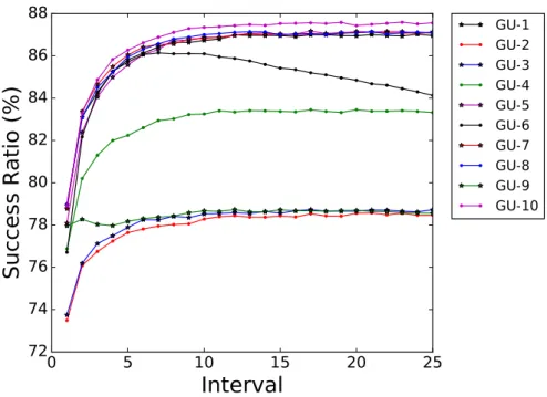
4.3.6.1 Pheromone Calculation GU-1 . . . 53
4.3.6.2 Pheromone Calculation GU-2 . . . 53
4.3.6.3 Pheromone Calculation GU-3 . . . 54
4.3.6.4 Pheromone Calculation GU-4 . . . 54
4.3.6.5 Pheromone Calculation GU-5 . . . 54
4.3.6.6 Pheromone Calculation GU-6 . . . 54
4.3.6.7 Pheromone Calculation GU-7 . . . 55
4.3.6.8 Pheromone Calculation GU-8 . . . 55
4.3.6.9 Pheromone Calculation GU-9 . . . 55
4.3.6.10 Pheromone Calculation GU-10 . . . 56
4.4 Upper Confidence Bound Routing and Wavelength Assignment . . . . 56
4.4.1 Introduction . . . 56
4.4.2 Routing Table . . . 57
4.4.3 Initialisation . . . 58
4.4.4 Routing and Wavelength Assignment . . . 58
4.4.5 Global Update . . . 60
4.5 Conclusion . . . 60
5 EVALUATION ON FIXED GRID 62 5.1 Introduction . . . 62 5.2 Experimental Procedure . . . 62 5.2.1 Performance Measures . . . 63 5.2.2 Network Topologies . . . 63 5.2.3 Comparison Algorithms . . . 65 5.2.4 Procedure . . . 66
5.3.1 Comparison of FSAC Pheromone Calculations . . . 67
5.3.1.1 Relative Performance of Pheromone Calculations . . 67
5.3.1.2 Timewise Performance of Pheromone Calculations . . 69
5.3.1.3 Overall Performance of Pheromone Calculations . . . 72
5.3.2 Comparison Against Existing Algorithms . . . 73
5.3.2.1 Relative Performance Comparison . . . 73
5.3.2.2 Timewise Performance Comparison . . . 74
5.3.2.3 Overall Performance Analysis . . . 77
5.4 Medium Topology Results . . . 78
5.4.1 Comparison of FSAC Pheromone Calculations . . . 78
5.4.1.1 Relative Performance of Pheromone Calculations . . 78
5.4.1.2 Timewise Performance of Pheromone Calculations . . 80
5.4.1.3 Overall Performance of Pheromone Calculations . . . 82
5.4.2 Comparison Against Existing Algorithms . . . 83
5.4.2.1 Relative Performance Comparison . . . 84
5.4.2.2 Timewise Performance Comparison . . . 85
5.4.2.3 Overall Performance Analysis . . . 88
5.5 Large Topology Results . . . 89
5.5.1 Comparison of FSAC Pheromone Calculations . . . 90
5.5.1.1 Relative Performance of Pheromone Calculations . . 90
5.5.1.2 Timewise Performance of Pheromone Calculations . . 91
5.5.1.3 Overall Performance of Pheromone Calculations . . . 94
5.5.2 Comparison Against Existing Algorithms . . . 95
5.5.2.1 Relative Performance Comparison . . . 95
5.5.2.2 Timewise Performance Comparison . . . 97
5.5.2.3 Overall Performance Analysis . . . 100
5.6 Umbrella Analysis . . . 101
6.1 Introduction . . . 104 6.2 Experimental Procedure . . . 105 6.2.1 Performance Measures . . . 105 6.2.2 Network Topologies . . . 106 6.2.3 Comparison Algorithms . . . 107 6.2.4 Procedure . . . 108
6.3 Small Topology Results . . . 110
6.3.1 Comparison of FSAC Pheromone Calculations . . . 110
6.3.1.1 Relative Performance of Pheromone Calculations . . 110
6.3.1.2 Timewise Performance of Pheromone Calculations . . 112
6.3.1.3 Overall Performance of Pheromone Calculations . . . 115
6.3.2 Comparison Against Existing Algorithms . . . 115
6.3.2.1 Relative Performance Comparison . . . 115
6.3.2.2 Timewise Performance Comparison . . . 116
6.3.2.3 Overall Performance Analysis . . . 119
6.4 Medium Topology Results . . . 121
6.4.1 Comparison of FSAC Pheromone Calculations . . . 121
6.4.1.1 Relative Performance of Pheromone Calculations . . 121
6.4.1.2 Timewise Performance of Pheromone Calculations . . 122
6.4.1.3 Overall Performance of Pheromone Calculations . . . 125
6.4.2 Comparison Against Existing Algorithms . . . 126
6.4.2.1 Relative Performance Comparison . . . 126
6.4.2.2 Timewise Performance Comparison . . . 127
6.4.2.3 Overall Performance Analysis . . . 130
6.5 Large Topology Results . . . 131
6.5.1 Comparison of FSAC Pheromone Calculations . . . 131
6.5.1.1 Relative Performance of Pheromone Calculations . . 132
6.5.2 Comparison Against Existing Algorithms . . . 136
6.5.2.1 Relative Performance Comparison . . . 137
6.5.2.2 Timewise Performance Comparison . . . 138
6.5.2.3 Overall Performance Analysis . . . 142
6.6 Umbrella Analysis . . . 142
6.7 Conclusion . . . 144
7 CONCLUSION 145 7.1 Introduction . . . 145
7.2 Overview of Results and Outcomes of Research Objectives . . . 145
7.3 Contributions . . . 147
7.4 Limitations . . . 150
7.5 Recommendation for Future Investigation . . . 150
7.6 Summary . . . 151
Appendices 161
A Appendix FSAC Fixed Grid Dataset 162 B Appendix FSAC Flexible Spectrum Dataset 169 C Appendix Fixed Grid Comparison Dataset 176 D Appendix Flexible Spectrum Comparison Dataset 180
E IEEE (SSCI) 2016 Paper 184
List of Figures
2.1 Available optical channels for a path composed of two links that
sat-isfy the WCC (Shen and Yang, 2011). . . 13
2.2 Frequency grid structures for Fixed, Flexi-Grid and Grid-Less (Flex-ible Spectrum) (Shen and Yang, 2011). . . 22
2.3 Spectrum Continuity of established paths(Capucho and Resendo, 2013). 24 2.4 Available spectrum for a route between nodes A and E (Wright et al., 2013). . . 26
2.5 Spectrum fragmentation over a network’s lifespan (Wright et al., 2013). 27 3.1 Shortest Path Finding capability of ant colonies (Blum, 2007). . . 33
5.1 Small 6-Node network topology . . . 64
5.2 Medium 11-Node network topology . . . 64
5.3 Large 14-Node network topology . . . 65
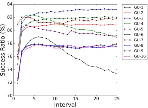
5.4 Burst Success Ratio for FSAC PCs on the small network topology with 8 wavelengths. . . 68
5.5 Burst Success Ratio for FSAC PCs over time at a load of 15. . . 69
5.6 Burst Success Ratio for FSAC PCs over time at a load of 30. . . 70
5.7 Burst Success Ratio for FSAC PCs over time at a load of 45. . . 71
5.8 Burst Success Ratio on the small network topology with 8 wavelengths. 73 5.9 Burst Success Ratio over time at a load of 15. . . 75
5.10 Burst Success Ratio over time at a load of 30. . . 76
5.11 Burst Success Ratio for FSAC PCs over time at a load of 45. . . 77
with 12 wavelengths. . . 79
5.13 Burst Success Ratio for FSAC PCs over time at a load of 20. . . 81
5.14 Burst Success Ratio for FSAC PCs over time at a load of 40. . . 82
5.15 Burst Success Ratio for FSAC PCs over time at a load of 60. . . 83
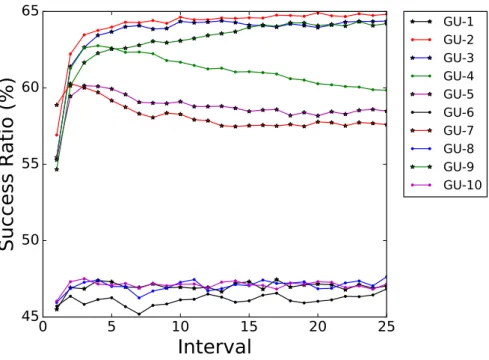
5.16 Burst Success Ratio on the medium network topology with 12 wave-lengths. . . 84
5.17 Burst Success Ratio over time at a load of 20. . . 86
5.18 Burst Success Ratio over time at a load of 40. . . 87
5.19 Burst Success Ratio over time at a load of 60. . . 88
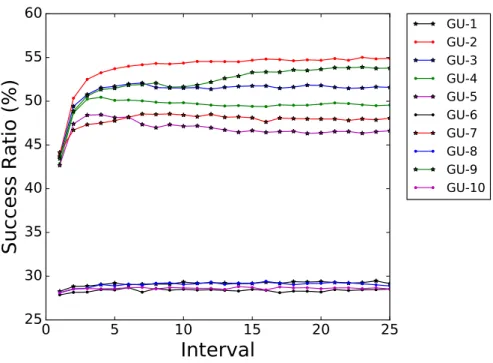
5.20 Burst Success Ratio for FSAC PCs on the large network topology with 16 wavelengths. . . 90
5.21 Burst Success Ratio for FSAC PCs over time at a load of 20. . . 92
5.22 Burst Success Ratio for FSAC PCs over time at a load of 40. . . 93
5.23 Burst Success Ratio for FSAC PCs over time at a load of 60. . . 94
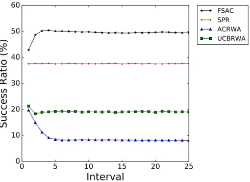
5.24 Burst Success Ratio on the large network topology with 16 wavelengths. 95 5.25 Burst Success Ratio over time at a load of 20. . . 97
5.26 Burst Success Ratio over time at a load of 40. . . 98
5.27 Burst Success Ratio over time at a load of 60. . . 99
6.1 Small 6-Node network topology . . . 106
6.2 Medium 11-Node network topology . . . 107
6.3 Large 14-Node network topology . . . 108
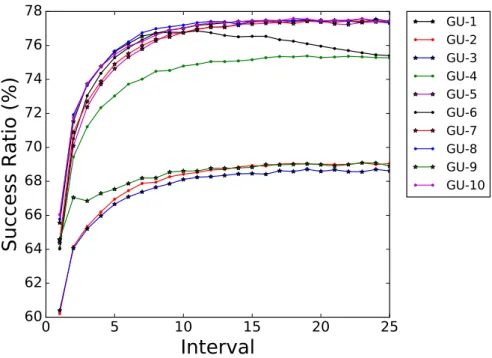
6.4 Burst Success Ratio for FSAC PCs on the small network topology. . . 111
6.5 Burst Success Ratio for FSAC PCs over time at a load of 30. . . 112
6.6 Burst Success Ratio for FSAC PCs over time at a load of 60. . . 113
6.7 Burst Success Ratio for FSAC PCs over time at a load of 90. . . 114
6.8 Burst Success Ratio on the small network topology. . . 116
6.11 Burst Success Ratio over time at a load of 90. . . 120
6.12 Burst Success Ratio for FSAC PCs on the medium network topology. 121 6.13 Burst Success Ratio for FSAC PCs over time at a load of 30. . . 123
6.14 Burst Success Ratio for FSAC PCs over time at a load of 60. . . 124
6.15 Burst Success Ratio for FSAC PCs over time at a load of 90. . . 125
6.16 Burst Success Ratio on the medium network topology. . . 126
6.17 Burst Success Ratio over time at a load of 30. . . 128
6.18 Burst Success Ratio over time at a load of 60. . . 129
6.19 Burst Success Ratio over time at a load of 90. . . 130
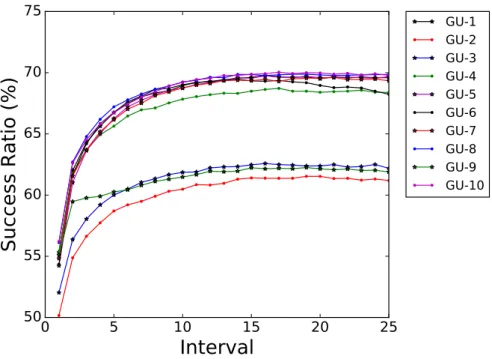
6.20 Burst Success Ratio for FSAC PCs on the large network topology. . . 132
6.21 Burst Success Ratio for FSAC PCs over time at a load of 30. . . 134
6.22 Burst Success Ratio for FSAC PCs over time at a load of 60. . . 135
6.23 Burst Success Ratio for FSAC PCs over time at a load of 90. . . 136
6.24 Burst Success Ratio on the large network topology. . . 137
6.25 Burst Success Ratio over time at a load of 30. . . 139
6.26 Burst Success Ratio over time at a load of 60. . . 140
List of Tables
3.1 ACRWA Pheromone Table (Triay and Cervello-Pastor, 2010) . . . 38
4.1 FSAC Pheromone Table for node A, P TA. . . 49
4.2 Routing Table . . . 58
5.1 Overall performance of the FSAC PCs on the small network topology with 8 wavelengths. . . 72 5.2 Success ratio and 95% confidence interval at a specific load on the
small network topology with 8 wavelengths. . . 74 5.3 Overall Algorithm performance on the small network topology with
8 wavelengths. . . 74 5.4 Overall performance of the FSAC PCs on the medium network
topol-ogy with 12 wavelengths. . . 80 5.5 Success ratio and 95% confidence interval at a specific load on the
medium network topology with 12 wavelengths. . . 85 5.6 Overall Algorithm performance on the medium network topology with
12 wavelengths. . . 85 5.7 Overall performance of the FSAC PCs on the large network topology
with 16 wavelengths. . . 91 5.8 Success ratio and 95% confidence interval at a specific load on the
large network topology with 16 wavelengths. . . 96 5.9 Overall Algorithm performance on the large network topology with
16 wavelengths. . . 96
topologies. . . 101 5.11 Overall Algorithm performance on all the tested network topologies. . 101
6.1 Overall performance of the FSAC PCs on the small network topology. 110 6.2 Success ratio and 95% confidence interval at a specific load on the
small network topology. . . 117 6.3 Overall Algorithm performance on the small network topology. . . 117 6.4 Overall performance of the FSAC PCs on the medium network topology.122 6.5 Success ratio and 95% confidence interval at a specific load on the
medium network topology. . . 127 6.6 Overall Algorithm performance on the medium network topology. . . 127 6.7 Overall performance of the FSAC PCs on the large network topology. 133 6.8 Success ratio and 95% confidence interval at a specific load on the
large network topology. . . 138 6.9 Overall Algorithm performance on the large network topology. . . 138 6.10 Overall Pheromone Calculation performance on all the tested network
topologies. . . 143 6.11 Overall Algorithm performance on all the tested network topologies. . 143
A.1 Fixed Grid dataset of the Success ratio for FSAC PCs on the small network topology . . . 163 A.2 Fixed Grid dataset of the Success ratio for FSAC PCs on the medium
network topology . . . 165 A.3 Fixed Grid dataset of the Success ratio for FSAC PCs on the large
network topology . . . 167
B.1 Flexible Spectrum dataset of the Success ratio for FSAC PCs on the small network topology . . . 170
medium network topology . . . 172 B.3 Flexible Spectrum dataset of the Success ratio for FSAC PCs on the
large network topology . . . 174
C.1 Fixed Grid dataset of the Success ratio for all the tested algorithms on the small network topology . . . 176 C.2 Fixed Grid dataset of the Success ratio for all the tested algorithms
on the medium network topology . . . 177 C.3 Fixed Grid dataset of the Success ratio for all the tested algorithms
on the large network topology . . . 178
D.1 Flexible Spectrum dataset of the Success ratio for all the tested algo-rithms on the small network topology . . . 180 D.2 Flexible Spectrum dataset of the Success ratio for all the tested
algo-rithms on the medium network topology . . . 181 D.3 Flexible Spectrum dataset of the Success ratio for all the tested
Abbreviation Term
ACO Ant Colony Optimisation
UCB Upper Confidence Bound
RWA Routing and Wavelength Assignment
RSA Routing and Spectrum Assignment
WCC Wavelength Continuity Constraint
SCC Spectrum Continuity Constraint
OCS Optical Circuit Switching
OPS Optical Packet Switching
OBS Optical Burst Switching
WDM Wavelength Division Multiplexing
DWDM Dense Wavelength Division Multiplexing
BCP Burst Control Packet
BCP-RA Burst Control Packet Release Acknowledgement
BCP-FA Burst Control Packet Failure Acknowledgement
BCP-TA Burst Control Packet Traversal Acknowledgement
ITU International Telecommunication Union
PLI Physical Layer Impairment
JIT Just-In-Time
JET Just-Enough-Time
SPR Shortest Path Routing
ACRWA Ant Colony Routing and Wavelength Assignment
UCBRWA Upper Confidence Bound Routing and Wavelength Assignment
Chapter 1
RESEARCH CONTEXT
1.1
Introduction
There is an ever growing demand for more bandwidth in optical transport networks (Yao et al., 2000). The telecommunication industry has been forced to upgrade its infrastructure and seek out new techniques to increase the capacity of optical transport networks (Imran and Aziz, 2014). Advances in Wavelength Division Mul-tiplexing (WDM) technology has dramatically increased the network capacity (Yao et al., 2000). There is an increasingly growing amount of traffic driven by the high-definition video distribution services, cloud computing among many others with increasing high-speed broadband penetration through both fixed and mobile termi-nals (Wright et al., 2013; Jinno et al., 2009). Research is required to address the demand for more bandwidth.
1.2
Background
Current optical networks primarily employ Optical Circuit Switching (OCS) which is well suited for persistent high bandwidth traffic that does not vary much over time (Ngo et al., 2006). In OCS networks, an all optical path between the source and destination node is established prior to the transmission of data in a static
manner (Jue et al., 2009). The bandwidth is not efficiently utilised as the resources are reserved when not in use, especially when carrying varying traffic over time (Jue et al., 2009).
Optical Packet Switching (OPS) and Optical Burst Switching (OBS) are optical switching technologies developed to overcome the static and inefficient allocation of network resources by existing OCS networks (Agrawal et al., 2005). OBS is a technical compromise between OCS and OPS in a flexible yet feasible way as it does not require optical buffering or packet-level processing as is the case with OPS (Galdino et al., 2010). OBS is a technology that offers a more flexible and dynamic optical network compared to traditional OCS networks. However, OBS does suffer from burst losses due to a lack of cost effective optical buffers and resource reservation schemes. The Routing and Wavelength Assignment (RWA) process is especially difficult in an optical network with no wavelength converters and buffers within the core increasing the risk of burst losses.
Ant Colony Optimisation (ACO) algorithms have been extensively applied to solve routing problems within telecommunication networks (Ngo et al., 2006). ACO is a biologically inspired system based on the social and foraging behaviour patterns of ants seeking an optimal path between their food source and colony (Dorigo and Di Caro, 1999). This behaviour has been imitated and adapted for use in solving various graph based computational problems. Several ACO algorithms have been used for solving the routing and wavelengths assignment problem in OBS networks (Triay and Cervello-Pastor, 2009; Pedro et al., 2009; Donato et al., 2012). ACO is of particular interest as it is able to run continuously, adapting to changes in the network state and traffic load in real time which provides a dynamic solution to the RWA problem.
Currently, optical channels are fixed, providing a reliable solution which mini-mizes inter-channel collisions and crosstalk. This however, limits the performance and flexibility of the optical network. There is thus a requirement for more advanced approaches toward more spectrum-efficient technologies(Shen and Yang, 2011; Wen
et al., 2013). A promising alternative is represented by flexible optical network-ing which is expected to provide enhanced spectrum management with respect to the Fixed Grid of traditional WDM systems and be able to “scale to match” the capacity requirements of future systems (Manousakis and Ellinas, 2016). The flex-ible component refers to the ability of the optical network to dynamically adjust its optical resources in an optimum and elastic way according to the continuously varying traffic conditions and demands (Waldman et al., 2013). Flexible Spectrum offers a flexible and dynamic spectrum assignment solution in order to effectively increase the capacity in optical transport networks (Capucho and Resendo, 2013; Klinkowski and Walkowiak, 2011). There is a potential penalty associated with the use of Flexible Spectrum. The removal of the traditional International Telecom-munication Union (ITU) Fixed Grid to improve spectrum utilization can possibly increase the effects of transmission impairments. Therefore, a requirement for the effective management and utilization of the network resources is needed.
1.3
Motivation
The bandwidth demand is increasing in optical networks. Currently used techniques do not use full potential of optical networks. OBS is one of the most promising pro-posed optical switching techniques to exploit the advantages of optical communica-tion networks (Aguas et al., 2015). In the last few years, OBS has been successfully implemented on a number of testbeds demonstrating the architecture and protocols (Barpanda et al., 2014). OBS is the most likely optical switching technique to be implemented in the near future (Coulibaly et al., 2015).
With the introduction of higher transmission rates and various modulations, the traditional ITU Fixed Grid approach is unable to efficiently utilise bandwidth. The fixed channel spacing is able to achieve high capacity optical transmissions with larger channel spacing. However, bandwidth efficiency is decreased when a mix of transmission rates are used (Chino et al., 2016). Flexible Spectrum is able to
increase the spectral efficiency (Amar et al., 2014).
Flexible Spectrum is a promising approach, but it does come with a potential cost. Transmissions have the potential for impairment with respect to the increased traffic and lack of large channel spacing. Proposed routing algorithms should be aware of the linear and non-linear Physical Layer Impairments (PLIs) in order to operate closer to optimum performance (Johannisson and Agrell, 2014).
1.4
Research Objectives
The previous section provided a brief motivation for this study, the following research objectives were identified:
• Improve on current algorithms for OBS networks. This objective in-volves the development of new algorithms that are more effective than existing solutions.
• Provide for Flexible Spectrum in the developed approaches. The cur-rent OBS protocols and routing algorithms do not cater for Flexible Spectrum. The protocols and algorithms would need to be adapted in order to support this approach.
• Consider PLIs in Flexible Spectrum. Current research is mainly con-ducted on idealised scenarios which do not accurately represent the real world. This research investigates the more realistic scenarios in which PLIs are taken into account.
• Evaluate and refine the proposed ACO-based approaches. The final objective of this study is to evaluate the newly created algorithms in order to determine whether the previous objectives were achieved and to measure the contribution of this study.
The next section is concerned with the process that was followed to achieve this research.
1.5
Methodology
A literature study was performed on ACO and ACO-based approaches for RWA in optical networks, focusing on OBS. Flexible Spectrum was identified as a promis-ing approach toward improved spectral efficiency, however, there is a potential for transmission impairments due to linear and non-linear effects. A method for mod-elling PLI’s in Flexible Spectrum was identified and used in simulation. Appropriate ACO-based approaches were investigated, adapted for use in Flexible Spectrum and implemented. It was noted that the investigated ACO-based approaches were not successful in the Flexible Spectrum environment. In conclusion, the approaches were not able find and repeatedly make use of good solutions.
An investigation into the use of a route and wavelength combination was con-ducted to overcome this problem. This enforced the establishment and use of com-plete paths for greedy exploitation in Flexible Spectrum. The results obtained form this approach displayed an improvement over the initial ACO-based implementa-tions. The use of a route and wavelength combination differed from traditional ACO-based approaches. New pheromone calculation equations were proposed for the use of route and wavelength combinations, leading to the development of the novel Flexible Spectrum Ant Colony approach. Further investigation into the use of Upper Confidence Bound (UCB) to provide a balance between the exploration and exploitation in the RWA process was also conducted. A hybridisation of UCB and ACO lead to the development of the novel UCBRWA approach to select an appropriate route and wavelength combination for the RWA process.
The novel proposed approaches were tested and experiments conducted com-paring with and against existing algorithms (a simple greedy and an ant based algorithm) in a traditional ITU Fixed Grid and Flexible Spectrum scenario on three
different network topologies.
1.6
Scope
The scope of this research does not include an exhaustive parameter study. There are many parameters to test that could potentially impact the performance of the al-gorithms tested in this research significantly. The parameters used in this study were informed through the parameters used by other researchers, determined through a series of preliminary experiments, and expert knowledge.
1.7
Dissertation Layout
Chapters 2 and 3 present the the background to the problem statement, introducing the relevant literature and motivations for the proposed approaches. The proposed approaches are introduced and discussed in detail within Chapter 4. Chapters 5 and 6 discuss the experimental work conducted in order to measure the proposed approaches against existing algorithms. Details of the experimental method are presented and discussed within each chapter. Chapter 7 presents the conclusions drawn from this work. The chapters address the following issues:
• Chapter 2: The applicable background theory of Optical Networks, RWA, Optical Switching techniques, Flexible Spectrum and PLIs are discussed.
• Chapter 3: Related work and literature of ACO-based algorithms for RWA are presented. The application of UCB is detailed.
• Chapter 4: The developed novel ACO-based approaches FSAC and UCBRWA are presented and discussed. New pheromone calculations are explored for the use of routing tuples. The adapted OBS reservation protocol for Flexible Spectrum is detailed.
• Chapter 5: This chapter covers the experimental work performed in an ex-isting technology (traditional ITU Fixed Grid). Experimental method are discussed and details of the experiments are provided. Results of the experi-mental work are presented and discussed comparing the proposed approaches with existing algorithms.
• Chapter 6: This chapter covers the experimental work performed in a fu-ture technology (Flexible Spectrum with PLIs). Experimental method are discussed and details of the experiments are provided. Results of the experi-mental work are presented and discussed comparing the proposed approaches with existing algorithms.
• Chapter 7: In this chapter an overview is presented of the experimental work together with discussions and outcomes of the research objectives. The contributions and limitations of this work are detailed with recommendations for future research proposed.
• Appendix A: Presents the tabulated results collected for the FSAC algorithm pheromone updates on Fixed Grid.
• Appendix B: Presents the tabulated results collected for the FSAC algorithm pheromone updates on Flexible Spectrum.
• Appendix C: Presents the tabulated results collected for proposed approaches and existing algorithms on Fixed Grid.
• Appendix D: Presents the tabulated results collected for proposed approaches and existing algorithms on Flexible Spectrum.
• Appendix E: The conference paper that was accepted and presented at the 2016 IEEE Symposium Series on Computational Intelligence (IEEE SSCI 2016).
• Appendix F: The journal paper that was submitted to Photonic Network Communications and is under review.
Chapter 2
BACKGROUND AND
PROBLEM DESCRIPTION
2.1
Introduction
This chapter will discuss Optical Networks, past and present (Section 2.2). Routing (Section 2.3) covers the process of allocating a route and wavelength for an incoming transmission request in an optical network, introducing the importance of the WCC and presenting rudimentary methods for RWA. Current techniques for the trans-mission of data within optical networks is discussed in Section 2.4, introducing new optical switching techniques that have been proposed to make more efficient use of optical network resources than the current OCS technique. A detailed description of OBS and the manner in which it functions is provided in Section 2.4.2. Section 2.5 details new techniques developed for optical networks to enhance the manner in which optical spectrum is allocated, moving from the traditional ITU Fixed Grid to Flexi-Grid and Grid-Less (Flexible Spectrum) techniques. The above mentioned techniques, Flexi-Grid and Grid-Less, better cater for the use of mixed transmis-sion rates and modulations. The process of allocating a route and spectrum for an incoming transmission request in Flexible Spectrum is be covered, including the
importance of the SCC and the challenges Flexible Spectrum introduces in terms of Spectrum Fragmentation and PLIs. A detailed description of the PLIs covering the linear and non-linear impairments is provided, including an equation for modelling the associated effects in Section 2.6.
2.2
Optical Networks
An optical network is a high capacity telecommunication network that is based on optical technology and components. The optical network is composed of a collection of nodes and switches which are connected by means of optical fiber. Driven by the sustained growth of data traffic volume, a new approach is required to fulfil the traf-fic demands placed upon the optical network. Due to the limitations in technology at the time, signal frequencies had to be widely separated. The fused biconic tapered coupler system typically made use of 1310 nm and 1550 nm (1310 nm, 1500 nm and 1625 nm bands have very low signal loss) signals providing 5 Gb/s on a single fiber (Bourouha et al., 2002). This system provided double the bandwidth, in contrast to modern networks which can transmit an individual signal at 10 Gb/s and have several different signals transmitting at such a rate through the optical fiber simul-taneously (Bourouha et al., 2002). Due to advancements in technology however, the number of wavelengths will continue to increase (Wright et al., 2013). There are a few technological solutions which enable optical networks to meet the required bandwidth and flexibility for increased traffic demands. WDM was introduced to provide optical networks with additional capacity on existing optical fibers. Multi-plexing is the process of combining several different wavelengths in a single optical fiber and then separating them at the receiving end by means of de-multiplexing. A light detector or receiver is then required for each of the de-multiplexed wavelengths in order to convert the signal back into useful information. The WDM technique allows for the better utilisation of bandwidth within an optical fiber and overcomes the optoelectronic bottleneck by performing routing in the network nodes (Barpanda
et al., 2009). Each wavelength of each fiber link then becomes a sub-channel that is independent of the other wavelengths (Fernando et al., 2013).
Dense Wavelength Division Multiplexing (DWDM) has provided the core net-work capacity required by netnet-work operators for the past 15 years to maintain the exponential growth in bandwidth demand. The bandwidth of an optical fiber has been divided into a choice of either 100, 50 or even 25 GHz fixed spaced channels providing high capacity transport (Chen et al., 2014). The channel spacing allows for up to 160 optical channels to be utilised. The fixed grids have allowed net-work operators to serve the traffic growth well by either increasing the speed of the transponders on each channel or by moving to a denser grid spacing as the traffic levels have increased (Wright et al., 2013). DWDM systems, when compared to that of WDM, have had to maintain a finer and more stable transmission wave-length due to the finer granularity of the grid spacing. Granularity refers to the size of the spectrum channel spacing (Jinno et al., 2009). A standard grid has been successful in allowing vendors to develop components to the same specifications. An evenly spaced grid allows for simpler wavelength control and manufacture of de/multiplexing components. Technological improvements have allowed transpon-ders to increase transmission bit rates from 2.5 Gb/s per-wavelength to capacities of 10, 40 or even 100 Gb/s while still confining the signal to the 50 GHz channel grid spacing (Wright et al., 2013; Amaya et al., 2011).
2.3
Routing
This section introduces the RWA process, describing its application, presenting the importance of the WCC and further details rudimentary RWA methods.
2.3.1
Routing and Wavelength Assignment
The routing and wavelength allocation process establishes a path, a route and wave-length, in a network for a connection request. The problem of assigning the path is
referred to as the Routing and Wavelength Assignment (RWA) problem. The prob-lem consists of two distinct parts, computing a route from the source to destination node pair and then assigning an available wavelength (Barpanda et al., 2010). The RWA process has the goal of fulfilling the connection request, minimising the block-ing probability of future incomblock-ing requests and utilisblock-ing available network resources in an efficient manner (Siddiqui et al., 2004; Bhanja et al., 2010). The following are three forms of traffic generation for connection requests in optical networks:
• Static traffic is when all of the connections requests are known in advance, remain in the network for a long period of time and are not released once they have been setup.
• Incremental traffic have the connection requests arrive sequentially and remain in the network indefinitely.
• Dynamic traffic is when all of the connection requests arrive sequentially, are handled and routed one at a time where each of the connection requests remain in the network for a finite amount of time.
All discussed literature, experimental results and findings hereafter will be in terms of the Dynamic traffic generation. The RWA process determines the route and wavelength to assign to an incoming connection request for a particular source and destination node pair. Separating the RWA problem into two distinct parts, con-sider the routing component. The routing process calculates the route along which the incoming connection request will travel in order to reach the destination node (Siddiqui et al., 2004; Lin et al., 2008; Binh, 2008). Typically, the shortest route is selected as it would make use of the least optical resources. In a wavelength routed WDM network a link would have a fixed number of wavelengths in accor-dance with the fixed grid. The second component of the RWA process selects an available wavelength along the route chosen above. The wavelength routed WDM network may have no wavelength conversion at the intermediary nodes, therefore the selected path (route and wavelength) would need to satisfy the WCC.
The WCC forces the connection request to maintain the same wavelength through-out the rthrough-outing process which serves to avoid a costly optical-electrical conversion at the node level in order to alter a wavelength. In order to satisfy the WCC, the
Figure 2.1: Available optical channels for a path composed of two links that satisfy the WCC (Shen and Yang, 2011).
path must be bound to a single wavelength in order to traverse all the nodes along the selected path as seen in Figure 2.1. Figure 2.1 is an illustration of the currently reserved wavelengths on two links (Link 1 and Link 2). In Figure 2.1, the currently reserved wavelengths are displayed in colour while currently available wavelengths are represented as white space. The illustration at the bottom of Figure 2.1 is a representation of the combined reserved (represented in colour) and unreserved (rep-resented as white space) wavelengths on Link 1 and Link 2. Only the unreserved wavelengths (represented as white space) in the illustration at the bottom of Fig-ure 2.1 satisfy the WCC for a path composed of the two links. The allocation of a route and wavelength for a connection request must conform to the WCC (Binh, 2008; Durn et al., 2012). With this is mind, it is necessary to align both the RWA of a connection request in an integrated manner.
2.3.2
Rudimentary Assignment Processes
The RWA problem is usually simplified and separated into two distinct processes, a routing or path assignment and the wavelength assignment. There are many different routing assignment approaches. The following are three basic approaches to the routing assignment process:
• Fixed routing is a straightforward approach to the routing assignment process as there is only a single fixed route to make use of between the source and destination node pair. An example of this approach is Shortest Path Routing (SPR) which makes use of the shortest path between any source and destina-tion node pair. The shortest route for each source to node pair is calculated offline, typically using Dijkstras algorithm.
• The Fixed-Alternate routing approach makes use of multiple fixed routes be-tween the source and destination node pair. As a result, each node in the net-work must maintain a routing table of candidates for routes from the source to each destination. The candidates are typically made up of the shortest routes between the source and destination node pair. Typically, the alternate route does not share any links with the first or shortest path in the routing table.
• Adaptive routing is an approach that selects routes dynamically based on the current availability of wavelength on each of the links within the network. This approach requires current data on all the links within the network. Any feasible route, from source to destination node pair, can be a candidate for the routing process. The choice of route is determined by the approach, shortest-cost path first or least congested path first.
The wavelength assignment process is required to select a feasible wavelength for a given route from source to destination node pair. The wavelength assignment process can be performed either after or during the routing assignment process. There is the possibility of multiple available wavelengths to select. If no wavelengths are
available a new route must be selected or the request is blocked. The following are four basic approaches to the wavelength assignment process:
• The First-Fit wavelength assignment approach selects the first available wave-length by searching through an indexed list of wavewave-lengths. The approach iterates through the indexed list of wavelengths, considering the lower indexed wavelengths above those of the higher indexed wavelengths. This approach confines the existing connection within a small wavelength range, leaving a large number of wavelengths available for the longer routes.
• Random wavelength assignment is an approach which selects a wavelength from the set of available wavelengths on the source to destination node pair. This is performed by selecting at random one of the available wavelengths in the set, typically with a uniform probability. In a distributed scenario, Random wavelength assignment may outperform First-Fit as only limited and outdated information may be available.
• Most-Used wavelength assignment is a simple approach which determines the most used wavelength within the entire network. The approach then selects and assigns the most used wavelength to the incoming connection. The most used wavelength is selected in order to reduce the number of used wavelengths and promote maximum wavelength reuse in the network.
• The Least-Used wavelength assignment approach determines which is the least used wavelength within the entire network. The approach then selects and assigns the least used wavelength to the incoming connection. The least used wavelength is selected in order to evenly spread the load in the network across all the wavelengths.
A simple greedy algorithm for RWA is the combination of SPR with First-Fit wave-length assignment.
2.4
Optical Switching
This section introduces optical switching and different proposed optical switching techniques. A detailed description of OBS is presented followed by an introduction to optical switching reservation protocols.
2.4.1
Optical Switching Techniques
With an ever growing demand for more bandwidth in optical transport networks the telecommunication industry has been forced to upgrade its infrastructure and seek out new techniques to increase the capacity of optical transport networks (Imran and Aziz, 2014; Yao et al., 2000). Advances in WDM technology have dramatically increased the network capacity (Yao et al., 2000). Three optical switching techniques have been proposed to satisfy the requirements of current and future applications to satisfy the requirements of bandwidth-greedy application.
Optical networks primarily employ OCS as the current switching technique. In OCS networks, an all optical path between the source and destination node pair is established prior to the transmission of data in a static manner (Jue et al., 2009). The all optical path remains for the duration of transmission ensuring the full avail-ability of the bandwidth. OCS is well suited for persistent high bandwidth traffic that does not vary much over time (Ngo et al., 2006). The bandwidth is inefficiently utilised as the resources are reserved when not in use, especially when carrying vary-ing traffic over time (Jue et al., 2009). Internet traffic consists of a small number of large and long duration traffic flows and many small traffic flows (Hu et al., 2015). A requirement for the effective management and utilization of the network optical resources.
OPS and OBS techniques have been developed to address the bursty internet traffic (Hu et al., 2015). OPS is an optical switching technology developed to over-come the static and inefficient allocation of network resources by existing OCS net-works (Agrawal et al., 2005). OPS transmits the packets through the all optical
network on a packet-per-packet basis. The packet headers are processed and con-verted from optical to electronic. Meanwhile, the packet payloads are optically buffered until such time that the desired link is available. Current optical buffer technology is not sufficient enough to buffer large amounts of packets for any ex-tended period of time due to contention in the network leaving OPS as an excellent theoretical option for the future (Aguas et al., 2015).
The lack of feasible optical buffers and packet losses are the major limiting factors for OPS (Imran et al., 2016). Among the different proposed optical switching techniques, OBS is the most promising (Aguas et al., 2015). OBS is a technical compromise between OCS and OPS in a flexible yet feasible way as it does not require optical buffering or packet-level processing as is the case with OPS (Galdino et al., 2010). In OBS the bursts are transmitted in the optical domain throughout the network, this decreases the optical to electronic conversion and processing times (Aguas et al., 2015). This eliminates the need for buffers at the switching nodes by delaying the burst long enough for the Burst Control Packet (BCP) to be processed, which is sent prior to the burst (Hu et al., 2015). A major challenge for OBS is the reservation of optical resources, it is possible to ensure zero burst loss with two-way reservation (Imran et al., 2016). However, two-way reservation has the negative aspect of a comparatively long setup time.
2.4.2
Optical Burst Switching
OBS is an optical switching technique for transmitting bursts of traffic through the network only for the duration of the burst (Xu et al., 2001). The OBS optical switching paradigm is designed to achieve increased bandwidth flexibility with a lack of efficient optical buffers. In OBS, instead of converting and transmitting a single packet of data, the packets are aggregated into large chunks of data at the edge of the network and transmitted in the form of a burst (Papadimitriou et al., 2003; Galdino et al., 2010). The bursts of data are transmitted using a wavelength
channel and are switched through the core nodes of the network. These bursts are later disassembled at the destination node and its packets are delivered accordingly (Papadimitriou et al., 2003). Bursts of data are preceded by a BCP. The BCP for each burst is responsible for the resource reservation and is sent ahead of the data burst on a separate wavelength channel (Aydin et al., 2008). There is a delay between the BCP and the corresponding burst (Imran and Aziz, 2014). The delay allows the BCP to undergo optical to electronic and electronic to optical conversion at each intermediate node along the routing path of the burst (Chen et al., 2004). The intermediate nodes are then able to configure their switching matrix to direct the upcoming data burst to the available wavelength channel on the appropriate output link (Imran and Aziz, 2015). The burst is transmitted and switched without acknowledgement of resource reservations from the BCP (Rodrigues and Vaidya, 2009).
The BCP functions only to perform a set-up (reservation) request for optical resources, thereafter the source node transmits the burst (Imran and Aziz, 2014). Intermediate nodes perform the bandwidth reservation and switching immediately after receiving the BCP. As soon as the BCP is received by the switch, the switching elements are configured for the coming burst. Upon transmission of a data burst, the destination node transmits an acknowledgement to the source of the burst to acknowledge the successful or failed delivery thereof. The acknowledgement is the BCP Release Acknowledgement (BCP-RA) which is also responsible for deallocating optical resources. Until the intermediate node receives a BCP-RA, the switching elements will remain reserved (Kirci and Zaim, 2006). It is possible for multiple data bursts to contend at an intermediate node for the same bandwidths. Unresolved contention will lead to burst dropping and ultimately degrade network performance as bursts are switched all optically. In the case that the BCP is unable to reserve the required optical resources, the transmission is blocked, the node will create a BCP-RA in order to notify the source of the failure and to release the reserved optical resources. In the case that the BCP is able to reserve the optical resources and
the burst is successfully transmitted, the destination node will create a BCP-RA in order to notify the source of the success and to release the reserved optical resources.
2.4.3
Signalling Protocol
The two most popular signalling protocols for OBS are In-Time (JIT) and Just-Enough-Time (JET). The two protocols differ in that JIT will immediately reserve optical resources and explicitly release them, while JET delays the reservation of resources and then implicitly releases them (Kirci and Zaim, 2006).
In JIT, as soon as the BCP has been received and processed by a node it will immediately configure the optical switches for the incoming burst. Optical resources are reserved prior to the actual arrival of the incoming burst as no offset time is used (Kirci and Zaim, 2006). This contributes to a less efficient use of resources as the wavelengths are reserved prior to the burst arrival time and as a result the wavelength cannot be utilized until the corresponding burst has been sent. The manner in which the switching elements are configured can lead to increased burst loss.
Unlike JIT, JET makes use of offset time information that is contained within the BCP. JET functions by sending a BCP to the destination node containing the relevant offset time that is processed at each subsequent node. The offset time allows for the delayed reservation of optical resources by only configuring the optical switches at the node right before the arrival time of the burst (Kirci and Zaim, 2006). JET provides a protocol which makes more efficient utilization of optical resources with the cost of a more complex method.
2.5
Flexible Spectrum
This section introduces the Flexible Spectrum technique, the drive toward spectrum efficient techniques, the resource reservation process for Flexible Spectrum and some associated obstacles (the SCC and Spectrum Fragmentation).
2.5.1
Flexible Spectrum Drivers
There is still plenty of space to fit a 10 Gb/s directly modulated signal within a 50 GHz channel (Lord, 2014). It is more challenging to fit transmissions greater than or equal to 100 Gb/s within the 50 GHz channel. The Fixed Grid optical networks were designed on the premise that all traffic demands would have the same spectrum requirements. In order to fit the 100 Gb/s signal within a 50 GHz channel spacing it is necessary to modulate the signal, which could then only require the use of 37.5 GHz (Muoz et al., 2013; Lord, 2014). The rigid Fixed Grid approach is not ideal for the spectrum requirements of the long-reach transmission and high speed data rates of 400 Gb/s or higher. Modulation of the 400 Gb/s transmission cannot be accommodated within a 50 GHz channel (Amaya et al., 2011; Gerstel et al., 2012). A solution would be to increase the channel spacing of the Fixed Grid as a modulated 400 Gb/s transmission would require 150 GHz of spectrum (Muoz et al., 2013). It is however possible to demultiplex the 400 Gb/s transmission into four separate 100 Gb/s signals which could be accommodated within the 50 GHz channel spacing (Muoz et al., 2013; Wright et al., 2013). This method is wasteful and inefficient in terms of spectral utilisation.
With the increase of transmission rates, a 50 GHz fixed grid spacing would no longer be able to support future traffic growth (Wright et al., 2013). An option would be to convert to a 100 GHz fixed grid spacing. As mentioned above, this would be wasteful in terms of traffic demands that make use of lower transmission rates. It could be more beneficial to utilise a fixed grid comprised of different sized spectrum slots for different speed transponders. This would require an understanding of when and where traffic demands would take place at the design level of the network. A less rigid approach to the transmission rate allocation could be advantageous with respect to network capacity and efficiency.
Traditional optical networks strictly follow the traditional ITU Fixed Grid for wavelength spacing (Shen and Yang, 2011). These grids have a coarse granularity
which ultimately leads to non-optimal spectrum utilization (Yumer et al., 2014). The demands of exponential traffic growth and increased dynamic traffic have forced the creation of flexible and adaptive networks. The Flexible Spectrum technology addresses the above mentioned concerns.
2.5.2
Flexible Spectrum Approach
A Flexi-Grid network provides additional flexibility in terms of spectrum assignment through the combination of two concepts, namely, the use of a finer wavelength gran-ularity and the ability to concatenate adjacent wavelength slots together to form ar-bitrary sized spectrum channels (Yumer et al., 2014; Klinkowski et al., 2013). This approach allows for a finer match with respect to the required and provided spec-trum allocation for a transmission (Wright et al., 2013). Flexi-Grid improves the spectral utilization as compared to traditional WDM and DWDM networks using a Fixed Grid (Wen et al., 2013). The Flexi-Grid implementation replaces the rigid frequency grid with a more flexible structure, organised into a much finer granular-ity grid (Manousakis and Ellinas, 2016). Each transmission allocation is assigned an appropriate number of concatenated slots to form the required spectrum alloca-tion (Waldman et al., 2013; Capucho and Resendo, 2013; Klinkowski and Walkowiak, 2011). The key feature of Flexi-Grid is the manipulation of multiple contiguous sub-carrier wavelength slots, instead of independent wavelength channels. The Grid-Less (Flexible Spectrum) approach is a recent concept that does not follow the standard ITU Fixed Grid for wavelengths, as illustrated by Figure 2.2. In traditional WDM networks the granularity of the frequency spacing is typically coarse with frequency spacing ranges from 50 GHz and above. However, DWDM and Flexi-Grid networks will have a much finer frequency spacing granularity as small as 6.25 GHz (Wright et al., 2013). The Flexible Spectrum approach has no concept of a grid or frequency spacing, there is a continuous band of optical spectrum from which to use. Figure 2.2 illustrates the possible spectrum savings or improved spectral utilization between
Figure 2.2: Frequency grid structures for Fixed, Flexi-Grid and Grid-Less (Flexible Spectrum) (Shen and Yang, 2011).
the three technologies. The ITU Fixed Grid structure is rigid in spectrum assign-ment and can allocate far more spectrum resources than is necessary. The Flexi-Grid (Mini-grid in Figure 2.2) approach makes use of a finer granularity grid which is able to more efficiently allocate spectrum resources and illustrates significant spectrum savings over the standard ITU Fixed Grid structure (Shen and Yang, 2011; Zhang et al., 2011; Amaya et al., 2011). The Flexible Spectrum (referred to as Grid-Less in Figure 2.2) approach provides a more elastic method of spectrum allocation, making it a possible candidate for increase spectrum efficiency (Shen and Yang, 2011). The flexibility gain can only be made through a combination of key optical components and subsystems. Tunable laser sources and Wavelength Selective Switches (WSS) with a tunable central wavelength are required to make use of transmission tech-niques which allow for variable bandwidth allocation for a demand (Shen and Yang, 2011; Zhang et al., 2011; Klinkowski et al., 2013). The objective of the routing and spectrum allocation processes are to minimise the blocking probability of incoming and future traffic demands while optimally utilising the available spectrum. The ad-ditional flexibility within the network, namely the Flex-Grid and Flexible Spectrum approaches, create a challenge in controlling and managing the spectral resources (Wright et al., 2013). The use of arbitrary bandwidth channels further compounds the network blocking probability and can limit the network capacity due to spectrum
fragmentation (Wright et al., 2013).
2.5.3
Routing and Spectrum Assignment
The Routing and Spectrum Assignment (RSA) process is analogous to the RWA process described in Section 2.3.1. RSA and RWA share a key similarity in first calculating the route for the source to destination node pair for an incoming connec-tion request. In contrast with RWA, the RSA process is applied to a network that does not follow the standard ITU Fixed Grid. RSA is applied to a network with fine granularity for the spectrum grid (Flexi-Grid) or to a lack of grid altogether (Grid-Less). The second component of the RSA process would allocate a spectrum channel for the assigned route comprised of one or multiple frequency grid blocks for the Flexi-Grid network (Lord, 2014; Wright et al., 2013). Allocation of spectrum differs in the Grid-Less network,as an appropriate amount of bandwidth on a wave-length must be allocated in order to satisfy the incoming connection request (Takagi et al., 2011; Shen and Yang, 2011; Yin et al., 2013). RSA has a similar constraint to that of the WCC with respect to RWA, the RSA process is required to establish a path that occupies the same spectrum on all links along the source to destina-tion node pair (Capucho and Resendo, 2013; Klinkowski et al., 2013). The above mentioned concept is referred to as the Spectrum Continuity Constraint (SCC) as seen in Figure 2.3 which would apply to both the Flexi-Grid and Grid-Less spec-trum approaches. Figure 2.3 is an illustration of fulfilling five connection requests in a Flexi-Grid under the SCC and is referred to in the following text. The RSA process has allocated paths for four of the connection requests as illustrated by the multiple colours. Each of the paths have been allocated spectrum that satisfies the SCC. The fifth connection requests requires a total of three available contiguous frequency blocks between the source (node b) and destination (node d) node pair. The RSA process attempts to reserve the necessary spectrum along route b-c-d in-dicated with a light blue colour. However, only frequency slots 0-1-2 are available
Figure 2.3: Spectrum Continuity of established paths(Capucho and Resendo, 2013).
on link bc which accommodates the necessary spectrum requirements. There are six frequency blocks available on link cd, however, the available frequency blocks
5-6-7-8-9-10 cannot be allocated to the connection request as they do not satisfy the SCC. Frequency blocks0-1-2 on linkcd satisfy the SCC, but are currently in use to satisfy an existing connection request and are therefore unavailable. If the RSA process attempted to reserve the necessary spectrum along route b-e-d, there would be sufficient frequency blocks available on link be. Frequency blocks 0-1-2-3-4 on link ed are currently in use and as a result only frequency blocks 5-6 would satisfy the SCC. Route b-e-d cannot satisfy the connection request as it does not provide sufficient contiguous spectrum to the destination node.
The only feasible route that can satisfy the SCC for the fifth connection request is along b-a-f-e-d. There are four frequency blocks 7-8-9-10 available along all the links which provide sufficient contiguous spectrum along route b-a-f-e-d. Although the above reservation would satisfy the connection request, it would not be ideal as it is optical resource intensive. The construction and destruction of dynamic connections creates the isolated and non-contiguous bandwidth within the network’s available spectrum (Yin et al., 2013; Zhang et al., 2014). Integrating both the path calculation and spectrum allocation of connection requests within the RSA process is essential in reducing the fragmentation of available spectrum in the network. With this in mind, a less optical resource intensive solution could be achieved to satisfy the fifth connection request. It would be necessary to reprocess the third connection
request and reallocate the required spectrum. Frequency blocks 0-1-2-3-4 could be reallocated to 6-7-8-9-10, still satisfying the connection requests. The reallocation of connection request three would allow the fifth connection request to be routed along b-e-d as frequency blocks 0-1-2-3-4-5 are available and satisfy the SCC.
2.5.4
Spectrum Fragmentation
The transmission of a connection request from a source to destination node pair, requires that all the links along the route satisfy the SCC. This requirement is to avoid the costly electro-optical conversion at each of the nodes to change the wavelength of the transmission (Wright et al., 2013). Spectrum fragmentation is a side effect of dynamically altering spectrum allocations in a Flexi-Grid or Grid-Less environment. This fragmentation of the available spectrum bandwidth results in small spectral gaps that become unusable (Lord, 2014; Yin et al., 2013). The varied size of spectrum allocation for transmissions that exist in the Flexi-Grid and Grid-Less environments cause the spectrum to become isolated (Wen et al., 2013; Wright et al., 2013). The effect of spectrum fragmentation is illustrated in Figure 2.4. For example, a new connection request places a demand for 75 GHz of spectrum along route A to E. The RSA process allocates a path for the connection request. Inspection of the available spectrum along the allocated path reveals there is sufficient available spectrum to satisfy the requirements of the connection request. The available 75 GHz of spectrum is in the form of two non-contiguous spectrum blocks, 25 GHz and 50 GHz respectively. The RSA process is unable to allocate the a path to the connection request as the available spectrum is fragmented.
Without prior knowledge of the order in which traffic demands will be requested, network operators are unable to predict how network traffic will grow and how spec-trum will become fragmented. Future traffic demands are expected to be more dynamic. Network operators can use online approaches to reduce network fragmen-tation. A de-fragmentation scheme could be applied to all of the current
connec-Figure 2.4: Available spectrum for a route between nodes A and E (Wright et al., 2013).
tions on the network while it is still operational. This scheme would attempt to re-route and re-allocate the spectrum for the current connection in order to reduce the amount of isolated spectrum. This de-fragmentation scheme is not ideal as it would disrupt the network and customers. An improved approach would manage the spectrum fragmentation of the network within the RSA process. Handling the spectrum fragmentation during the RSA process would improve spectral efficiency and reduce the traffic blocking probability. This approach would limit the need to de-fragment the network spectrum globally, thereby limiting the disruption to the network and customers. Figure 2.5 illustrates the effect and risk of untreated spec-trum fragmentation over time within a network. Mismanagement of transmissions that are no longer required will leave spectral holes behind, causing the network to suffer from even greater spectrum fragmentation (Yin et al., 2013). It is possible that during a transmissions lifespan it may need to either increase or decrease its spectrum requirements. The use of bandwidth variable transponders allow a trans-mission demand to increase or decrease its spectrum requirement as the need arises
Figure 2.5: Spectrum fragmentation over a network’s lifespan (Wright et al., 2013).
(Wright et al., 2013). The spectrum made available from one transmission that is no longer required may be used to increase the bandwidth of another, provided the available spectrum is not isolated and forms a contiguous band with the current transmission.
2.6
Physical Layer Impairments
PLIs cause transmission impairments in optical networks. The linear and non-linear effects which cause impairments are introduced in the following section. A transmission penalty equation used to model linear and non-linear effects is detailed in Section 2.6.2.
2.6.1
Linear and Non-Linear Effects
PLIs are comprised of linear and non-linear effects. These effects increasingly de-teriorate the quality of transmissions with respect to an increase in transmission distance, bit-rates and various modulations. Optical fiber transmission are sus-ceptible to degradation due to several physical phenomena. In Flexible Spectrum networks, transmissions with various modulations and bandwidths can share the same fiber link (Yan et al., 2015b).
Linear impairments are independent of the signal power and affect each of the wavelengths (optical channels) individually. Attenuation and dispersion are impor-tant linear effects that limit transmission systems. Attenuation is the deterioration of signal strength through the traversal of optical fiber. Different wavelengths prop-agate at different speeds within the optical fiber that results in interference that leads to transmission errors.
The simultaneous transmission of multiple wavelengths through optical fiber af-fect not only each optical channel individually but they also cause disturbance and interference between them in the form of linear effects. The effects of non-linear impairments become crucial as data transmission rates, different modulation formats, transmission lengths, number of multiplexed wavelengths and transmis-sion intensities increase in addition to reduction in channel spacing. These linear and non-linear effects need to be effectively managed as they pose a serious risk within Flexible Spectrum networks. Network designers must be aware of these lim-itations and of the steps that can be taken to minimize the detrimental effects of these fiber non-linearities. To account for inter- and intra-channel interference in such networks, a realistic, yet tractable physical layer impairments (PLI) model is needed (Yan et al., 2015a). Thus, in todays optical networks it is imperative that appropriate care is taken to combat the crosstalk effect (Monoyios et al., 2016).
2.6.2
Transmission Penalty Equation
A novel part of this work, is that both linear and non-linear effects on the transmis-sions are taken into consideration. The transmistransmis-sions are affected by attenuation over the fiber and non-linear effects incurred by other transmissions simultaneously traversing the fiber. The signal channels are either separated by fixed channel spac-ing (Fixed Grid) or flexible spacspac-ing in the case of Flexible Spectrum. Dependspac-ing on the spacing, there arises crosstalk interferences between contiguous channels. The crosstalk is due to the non-linear effects as a result of the intensity dependence of
the refractive index of the fibre core (Agrawal, 2001). For multiple wavelengths, crosstalk is as a result of Cross-Phase Modulation leading to a non-linear phase change on channel 1 given by:
φ1 =γLef f(P1+P2) (2.1)
where γ is the non-linear coefficient due to the Kerr effect, Lef f is the effective
length where non-linear effects accumulate with the length of the fibre and P1 and
P2 are the powers of channel 1 and channel 2 respectively (Agrawal, 2001). The eventual outcome of crosstalk is that the signal receiver fails to distinguish closer wavelengths due to the incurred interference. With respect to a receiver sensitivity, the transmission penalty due to crosstalk can therefore be determined as the power difference in received signal power and the receiver sensitivity. Crosstalk depends on the signal bit-rate, channel spacing, received powers, length of the fibre and the band-pass filter bandwidth in the receiver (Agrawal, 2001). The crosstalk penalty can be quantified as the power ratio of the interfering signal that leaks into the desired channel to the signal channel power without crosstalk.
According to D.K. Boiyo (personal communication, April 27, 2015), the effects within the network and Flexible Spectrum environment can be replicated using a transmission penalty equation.
P enalty(dB) = AL+kL X i∈Tf\{s} Bs10 Pi 10 Bi10 Ps 10(fs−fi) (2.2)
where constant k = 4.78, A is the Line Attenuation in dB/km, L is equal to the length in km, Tf is the set of signals traversing the fibre link, Bs is the bit rate of
the signal in Mb/s, Bi is the bit rate of the signal causing the interference in Mb/s, Pi is the intensity of the signal causing the interference in dBm, Ps is the intensity
of the signal in dBm, (fs−fi) is the difference in central frequency of the signal and
the signal causing the interference in GHz.
The penalty on the intensity of a transmission is due to the simultaneous traversal of other transmissions and is calculated using equation (2.2). The result calculated