ISSN: 1992-8645 www.jatit.org E-ISSN: 1817-3195
573
INTER-TURN SHORT CIRCUIT FAULT DIAGNOSIS OF
INDUCTION MOTORS USING THE SVM OPTIMIZED BY
BARE-BONES PARTICLE SWARM OPTIMIZATION
PANPAN WANG, LIPING SHI
School of Information and Electrical Engineering, China University of Mining & Technology, Xuzhou
221008, Jiangsu, China
ABSTRACT
In order to accurately recognize the stator winding inter-turn short circuit fault of induction motors, a novel method for fault diagnosis was proposed based on a bare-bones particle swarm optimization algorithm (BBPSO) and support vector machine (SVM); and feasible diagnostic steps were also introduced. In this method, the feature vector of induction motor in different conditions was extracted with wavelet packet, and was considered as the input vector of SVM. The SVM was used to solve the classification problem, and the parameter-free BBPSO and cross-validation were taken to optimize model parameters, which avoided the blindness of parameter selection. Finally, the experiment shows that the proposed method is effective to diagnose the stator winding inter-turn short circuit fault of induction motors.
Keywords: Induction Motors, Stator Winding Inter-turn Short Circuit, Bare-Bones Particle Swarm Optimization, Support Vector Machine, Fault Diagnosis
1. INTRODUCTION
One of the most common faults is stator winding inter-turn short circuit, which covers approximately 30%~40% [1] of the overall fault conditions in induction motors. Therefore, early diagnosis of stator fault in induction motor is greatly significant.
The stator fault diagnosis of induction motors is a typical problem of pattern recognition. Recently, the method of pattern recognition mainly includes fuzzy theory [2], neural network [3], support vector machine (SVM) [4], etc. The first two methods are based on the statistical characteristics of large-scale samples. It is impossible to obtain good generalization properties when the number of training samples is insufficient. The SVM is a machine learning method based on statistical learning theory. It is especially suitable for classification, forecasting and estimation in small sample cases, and has been used widely for pattern recognition. However, the practicability of SVM is affected by the difficulty of selecting appropriate its parameters. Bare-bones particle swarm optimization (BBPSO) [5] which is a new global optimization technology was proposed by Kennedy. Compared with other optimization algorithms, the BBPSO has many advantages such as the simplicity, the parameter-free feature and the fast convergence.
In this paper, a method based on BBPSO and cross-validation was proposed to search the optimal SVM parameters. And then, the SVM optimized by BBPSO was applied to the winding inter-turn short circuit fault diagnosis of test motor to verify its validity, among which the feasible diagnostic steps were also introduced.
2. PARTICLESWARMOPTIMIZATION
ANDSVM
2.1Basic Particle Swarm Optimization
Particle swarm optimization (PSO) which was firstly proposed by Kennedy and Eberhart in 1995 is a stochastic, population-based optimization approach modeled after the simulation of social behavior of bird flocks [6]. In a PSO system, a swarm of individuals (called particles) fly through the search space. Each particle represents a candidate solution for the problem and adjusts its position by tracking two optima. One is its personal best position pi, namely, the best position found by
it so far. The other is the global best position pg,
namely, the best position found by its neighborhood particles so far. In each generation, the velocity vi=(vi,1, vi,2, …, vi,D) and position of particle xi=(xi,1, xi,2, …, xi,D) are updated by the following formulas,
574 )) ( ) ( ( )) ( ) ( ( ) ( ) 1 ( , , 2 2 , , 1 1 , , t x t p r c t x t p r c t wv t v j i j g j i j i j i j i − + − + = + (1) ) 1 ( ) ( ) 1 ( , ,
, t+ =x t +v t+
xij ij ij (2)
Where w is an inertia weight to control exploration in the search space, c1 and c2 are two
positive constants, r1 and r2 are two random
numbers within [0,1]. vi,j∈[−vmax,vmax], where
vmax is set by the user.
2.2Bare-Bones Particle Swarm Optimization
Clerc and Kennedy proved that each particle converges to a weighted average of its personal best and neighborhood best position [7], that is,
j j j g j j i j j i c c p c p c G , 2 , 1 , , 2 , , 1 , + +
= (3)
This theoretically derived behavior provides support for the bare-bones particle swarm optimization (BBPSO) developed by Kennedy. In BBPSO, the formula for updating particle’s velocity is eliminated, and a Gaussian sampling based on the pi and pg information is used as follows [5]
)) ( ), ( ( ) 1
( , 2,
, t N t t
xij + = µij σij (4)
Where µi,j(t)=(pi,j(t)+pg,j(t)) 2 and
) ( ) ( ) ( , , 2
,j t pij t pgj t
i = −
σ are the mean and
standard deviation of Gaussian distribution, respectively. Compared to the canonical PSO, BBPSO is obviously control parameter-free and more compact. So it is natural to apply it to some real application problems.
2.3Support Vector Machine
Support vector machine (SVM) was originally introduced to solve the two-classification problem in case of linearly separable [8]. Given a training set of l data points T =
{
xi,yi}
li=1, where xi∈Rd is thei-th input pattern with d dimensions and yi∈
{ }
−1,1 is the i-th output pattern. The SVM aim is to construct an optimal separating hyper-plane which can separate the data correctly and create the maximum distance between the plane and the nearest data. The corresponding constraint optimization problem is as follow.) , , 2 , 1 ( , 0 1 ) ( s.t. 2 1 min 1 , , l i b x w y C w w i i i T i l i i T b w = ≥ − ≥ + +
∑
= ξ ξ ξ ξ (5)Where C is a penalty factor, ξi is a slack factor.
Eq.(5) is a classical convex optimization problem. The calculation can be simplified by converting the problem with Kuhn-Tucker condition into the equivalent Lagrangian dual problem, which will be expressed as ) , , 2 , 1 ( , 0 0 s.t. ) ( 2 1 min 1 1 1 1 l i C y x x y y i i l i i l j j l i l j j i j i j i = ≤ ≤ = − ⋅
∑
∑
∑∑
= = = = α α α α α α (6)Thus, by solving this dual optimization problem, one obtains the optimum solution
) , , ,
( 1* 2* *
*
l
α α α
α = , and then calculates the
) ( 1 * * j i l i i i
j y x x
y
b = −
∑
⋅=
α . This leads to linear
decision function: ⋅ + =
∑
= l i i ii x x b
y x f 1 * * ) ( sgn )
( α (7)
For non-linearly separable cases, the original input pattern space is mapped into the high dimensional feature space through some non-linear mapping functions Φ:Rd →H . Thus, the non-linear problem in low dimensional space corresponds to the linear problem in the high dimensional space. And the SVM needs not to compute the inner product in the feature space. According to kernel function theory, we can use the kernel function K(xi,xj)=(Φ(xi)⋅Φ(xj)) in the
input space, which satisfies the Mercer condition, to compute the inner product. So the decision function can be expressed as
+ =
∑
= l i i ii K x x b
y x f 1 * * ) , ( sgn )
( α (8)
3. SVMPARAMETEROPTIMIZATION
ISSN: 1992-8645 www.jatit.org E-ISSN: 1817-3195
575 determine the kind of kernel function firstly. According to the analysis of literature [9], the SVM performance is better in non-linearly separable and small sample case, when the radial basis function (RBF) is selected as kernel function. Therefore, the RBF is also used in this paper, and it is of the form:
−
−
= 2
2
2 exp ) , (
σ
y x y
x
K (9)
Where σ is the bandwidth of the RBF kernel. It affects the mapping transformation of data space and alters the complexity degree of sample distribution in the higher dimensional feature space. The penalty factor C of Eq.(5) determines the trade-offs between the minimization of the fitting error and the minimization of the model complexity. If C and σ are not properly chosen, the SVM performance would be weakened. So the BBPSO is applied to optimize the SVM parameters. And the error of k-fold cross-validation is selected as fitness function, which is defined as:
∑
=
= k
i i
l l C
f
1
) ,
( σ (10)
Where li is the number of false-classification
sample in i-th testing set; l denotes the number of training samples.
The key steps for optimizing SVM parameters with BBPSO can be described as follows:
Step1 Preprocess the training data which
includes feature extraction based on wavelet packet and normalization.
Step2 Initialize particle position Pj(Cj, σj),
personal best position and global best position randomly; set the BBPSO parameters such as population size and maximum generation.
Step3 Calculate particle fitness. Firstly, divide the training set into k mutually exclusive subsets of approximately equal size (S1,S2,…,Sk). Select one
subset Si as testing set, the rest are used as training
set. Train SVM, and then calculate li. Repeat above
process k times, so that each subset is used once for validation. According to Eq.(10), calculate each particle fitness.
Step4 Update personal and global best position.
Step5 Update particle position according to
Eq.(4).
Step6 If the termination criteria are satisfied, stop the iteration procedure; otherwise, go to step3.
4. FEATUREEXTRACTIONAND
DIAGNOSISSTEPS
4.1Feature Extraction Based On Wavelet
Packet
When the inter-turn short circuit fault of induction motor appears, the stator asymmetry causes a rise of space harmonics. Therefore the spatial distribution of the flux density can not be considered sinusoidal. The interaction between the electrical quantities at the fundamental frequency and the different space harmonics produces additional time harmonic components in the stator currents. And the harmonic components of the stator current caused by the rotor slotting are also changed, when the stator winding is asymmetry [10,11].
In this fault condition, the stator inter-turn short circuit will change the energy distribution in the frequency bands of the stator current signal. Wavelet packet analysis is an effective time frequency analysis tool. It can decompose the original signal into independent frequency bands, and there is no redundant information in these frequency bands. So the inter-turn short circuit fault features of induction motor can be extracted from the stator current by using the wavelet packet analysis.
+ =
+
+ =
∑
∑
− −
k k l k l
k k l k l
n j d b n
j d
n j d a n j d
) , 1 ( )
1 2 , (
) , 1 ( )
2 , (
2 2
(11)
Where ak-2l and bk-2l are the coefficients of
wavelet packet filter banks. According to Parseval
equality 2
2
) , ( )
(
∑
∫
+∞ =∞
− f x dx d j k , the quadratic
sum of wavelet packet transform coefficients d(j,k) is equal to the energy of the original signal in the time domain. Hence, it is reliable to extract the energy feature from the original signal by using coefficients of wavelet packet transform.
4.2Fault Diagnosis Steps
Based on BBPSO and SVM, the fault diagnosis steps of stator inter-turn short circuit are described as follows:
Step 1: Decompose the current signal into j
layers wavelet coefficients, and then get M=2j independent frequency bands.
Step 2: According to Parseval equality, the
energy eigenvalue Ei(i=1,2,…,M) of each frequency
576
∑
=
= Ni
k i d i k
E 1
2
) ,
( (12)
where the Ni is the data length of the i-th frequency
band.
Step 3: Construct the eigenvector of fault feature as follow, and normalize it.
[
t t tM]
T= 1, 2,, (13)
Where
min , max ,
min ,
i i
i i i
E E
E E t
− −
= .
Step 4: Select T to be the input vector of the SVM, and divide the sample set into training subset and testing subset. Adopt BBPSO and cross-validation to sort the optimal parameters of SVM.
Step 5: Adopt the optimal parameters and
training set to construct SVM classifier.
Step 6 Using the trained SVM, classifier the
testing set.
5. EXPERIMENTALRESULTSAND
ANALYSIS
[image:4.612.320.509.348.651.2]The test bench used in the experimental investigation is available at the School of Information and Electrical Engineering in the CUMT. The Fig.1 shows the test bench.
Figure 1: The Experimental Test Bench
The type of test motor is Y132M-4. Tests were achieved by connecting an external shorting variable resistor Rx between terminals pairs to
introduce the short circuit fault. Adjusting the resistor can change the severity of the inter-turn short circuit fault, as shown in Fig.2.
Rx
A
B C
Figure 2: Stator A-Phase Winding Inter-Turn Short Circuit Loop
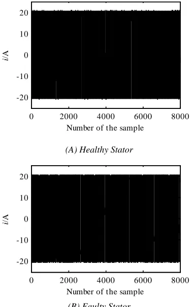
The detection tests were performed first using a healthy stator, then a faulty stator (Rx=20kΩ). The
sampling rate is 1666Hz and the number of samples per signal rises at 8000 samples. A total of 21 recordings per condition type are collected. Fig.3 presents the stator currents of two conditions in the time domain.
0 2000 4000 6000 8000
-20 -10 0 10 20
Number of the sample
i
/A
(A) Healthy Stator
0 2000 4000 6000 8000
-20 -10 0 10 20
Number of the sample
i
/A
(B) Faulty Stator
Figure 3: Waveforms Of Stator Current
[image:4.612.110.280.467.594.2]ISSN: 1992-8645 www.jatit.org E-ISSN: 1817-3195
577 Then the eigenvector of fault feature was constructed and normalized.
[image:5.612.95.293.200.235.2]In this experiment, we take 15*2 samples as training set, and 6*2 samples as testing set. Using the method in section 3, search the appropriate SVM parameters, among which k=3 and the BBPSO parameters are shown in Table I.
Table I: Parameter Configurations Of The BBPSO
Algorithm Population size Maximum generation
BBPSO 20 50
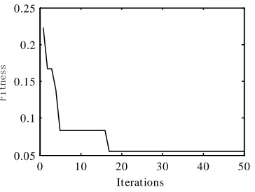
The BBPSO found the optimal SVM parameters Cbest=4.031 and σbest=1.497, and the error of 3-fold
cross-validation is 0.056. Fig.4 graphically presents the evolutionary process in solving the parameter selection problem.
0 10 20 30 40 50
0.05 0.1 0.15 0.2 0.25
Iterations
[image:5.612.320.516.240.324.2]Fitness
Figure 4: Fitness Evolutionary Curves
Training SVM with Cbest, σbest and training set,
[image:5.612.100.282.315.452.2]the SVM model for detecting stator fault is obtained. Then the testing samples are input into the trained model to validate its generalization performance. The classification results are shown in Table II. For two motor conditions, healthy stator and faulty stator, the target decision values of SVM are [svm>0] and [svm<0] respectively.
Table II Test Classification Results Of The Trained SVM
Testing samples SVM actual decision values
Classification results 1: healthy stator 1.491>0 healthy stator 2: healthy stator 0.399>0 healthy stator 3: healthy stator 1.174>0 healthy stator 4: healthy stator 1.204>0 healthy stator 5: healthy stator 0.526>0 healthy stator 6: healthy stator 0.151>0 healthy stator 7: faulty stator -1.025<0 faulty stator 8: faulty stator -0.886<0 faulty stator 9: faulty stator -0.785<0 faulty stator 10: faulty stator -1.683<0 faulty stator 11: faulty stator -1.378<0 faulty stator 12: faulty stator -0.916<0 faulty stator
From Table II, we can see that the SVM model of stator fault is accurate and has very strong ability of generalization. Although the number of training samples is only 30, the classification accuracy of the testing set is up to 100%.
In order to validate the superiority of optimal parameters, a comparison between SVM classifier with optimal parameters and ones with different parameters selected randomly is done. The comparison results are shown in Table III.
Table III: Svm Performance Comparison with Different Parameters
C σ
Classification accuracy of training set/%
Classification accuracy of testing set/%
4.031 1.497 100.0 100.0
1.000 1.497 94.4 91.7 15.000 1.497 100.0 100.0
4.031 0.150 77.8 75.0 4.031 25.000 100.0 100.0
Form Table III, it is clear that the values of C and σ are too large or too small, which will affect the SVM performance. When C=15.000, the classification accuracy is also up to 100%. But, larger C will often lead to appearance of over fitting and increase the model complexity. The optimal parameters (first group C and σ values) optimized by BBPSO improve the recognition accuracy obviously and reduce the blindness of parameter selection.
6. CONCLUSION
This paper proposes a new method based on BBPSO and SVM to diagnose stator inter-turn short circuit fault for induction motor. In the diagnosis method, the SVM is employed as the classifier and its parameters, C and σ, are optimized by proposed BBPSO approach. Experimental results show that the diagnosis method can correctly and effectively recognize the stator inter-turn short circuit fault for induction motor. Compared with several other SVMs with random parameters, it is higher precision ratio and reduces the blindness of parameter selection. Therefore, the proposed method can enhance induction motor safety and save maintenance cost.
REFRENCES:
[image:5.612.96.297.580.717.2]578 Meeting, IEEE Conference Publishing Services, October 03-07, 1999, pp. 197-204.
[2] H. Xie, X. Tong, “A method of synthetical fault diagnosis for power system based on fuzzy hierarchical Petri net”, Power System Technology, Vol. 36, No. 1, 2012, pp. 246-252.
[3] L. Zheng, S. Liu, X. Xie, “Modified wavelet neural network based nonlinear model identification for photovoltaic generation system”, Power System Technology, Vol. 35, No. 10, 2011, pp. 159-164.
[4] X. An, M. Zhao, D. Jiang, S. Li, “Direct-drive wind turbine fault diagnosis based on support vector machine and multi-source information”, Power System Technology, Vol. 35, No. 4, 2011, pp. 117-122.
[5] J. Kennedy, “Bare bones particle swarms”, Proceedings of IEEE Swarm Intelligence Symposium, IEEE Conference Publishing Services, April 24-26, 2003, pp. 80-87.
[6] J. Kennedy, R. C. Eberhart, “Particle swarm optimization”, Proceedings of IEEE International Conference on Neural Networks, IEEE Conference Publishing Services, November 27-December 01, 1995, pp. 1942-1948.
[7] M. Clerc, J. Kennedy, “The particle swarm-explosion, stability, and convergence in a multidimensional complex space”, IEEE Transactions on Evolutionary Computation, Vol. 6, No. 1, 2002, pp. 58-73.
[8] C. Cortes, V. Vapnik, “Support-vector, networks”, Machine Learning, Vol. 20, No. 1, 1995, pp. 273-295.
[9] J. Yang, Y. Zhang, R. Zhao, “Application of support vector machines in trend prediction of vibration signal of mechanical equipment”, Journal of Xi’an Jiao Tong University, Vol. 39, No. 9, 2005, pp. 950-953.
[10] S. Andreas, G. S. Howard, P. James, “Current monitoring for detecting inter-turn short circuits in induction motors”, IEEE Trans on Energy Conversion, Vol. 16, No. 1, 2001, pp. 32-37.