http://dx.doi.org/10.4236/am.2014.513192
How to cite this paper: EL-Sawy, A.A., Hussein, M.A., Zaki, E.-S.M. and Mousa, A.A. (2014) Local Search-Inspired Rough Sets for Improving Multiobjective Evolutionary Algorithm. Applied Mathematics, 5, 1993-2007.
http://dx.doi.org/10.4236/am.2014.513192
Local Search-Inspired Rough Sets for
Improving Multiobjective Evolutionary
Algorithm
Ahmed A. EL-Sawy1,2, Mohamed A. Hussein1*, El-Sayed Mohamed Zaki1, Abd Allah A. Mousa1,3
1Department of Basic Engineering Sciences, Faculty of Engineering, Menoufia University, Shibin El-Kom, Egypt 2Department of Mathematics, Faculty of Science, Qassim University, Buraydah, Saudi Arabia
3Department of Mathematics, Faculty of sciences, Taif University, Taif, Saudi Arabia Email: *[email protected]
Received 16 April 2014; revised 22 May 2014; accepted 5 June 2014
Copyright © 2014 by authors and Scientific Research Publishing Inc.
This work is licensed under the Creative Commons Attribution International License (CC BY). http://creativecommons.org/licenses/by/4.0/
Abstract
In this paper we present a new optimization algorithm, and the proposed algorithm operates in two phases. In the first one, multiobjective version of genetic algorithm is used as search engine in order to generate approximate true Pareto front. This algorithm is based on concept of co-evolu- tion and repair algorithm for handling nonlinear constraints. Also it maintains a finite-sized arc-hive of non-dominated solutions which gets iteratively updated in the presence of new solutions based on the concept of ε-dominance. Then, in the second stage, rough set theory is adopted as lo-cal search engine in order to improve the spread of the solutions found so far. The results, pro-vided by the proposed algorithm for benchmark problems, are promising when compared with exiting well-known algorithms. Also, our results suggest that our algorithm is better applicable for solving real-world application problems.
Keywords
Multiobjective Optimization, Genetic Algorithms, Rough Sets Theory
1. Introduction
Many real optimization problems require optimizing multiple conflicting objectives with each other. These problems with more than one objective are called Multiobjective Optimization Problems (MOPs). There is no
single optimal solution, but a set of alternative solutions; these solutions are optimal in the wider sense that no other solutions in the search space dominate them when all objectives are considered. They are known as Pareto optimal solutions [1] [2]. MOPs naturally arise in many area of knowledge such as economics [3]-[5], machine learning [6]-[8] and electrical power system [9]-[12].
Deb [13] classified optimization methods as classical (traditional) methods and evolutionary methods (evolu-tionary algorithms). Traditional multiobjective methods attempt to find the set of nondominated solutions using mathematical programming. In traditional methods such as weighted method and ε-constraint method which are most commonly used [1], the MOPs are transformed into a single objective problem which can be solved using nonlinear optimization techniques.
On the other hand, evolutionary methods (evolutionary algorithms EAs) for MOPs optimize all objectives si-multaneously and generate a set of alternative solutions. The simultaneous optimization can fit with population based approaches, such as EAs, because they generate multiple solutions in a single run. These population- based approaches are more successful when solving MOPs. There are many algorithms for solving uncon-strained MOPs. A representative collection of these algorithms includes the vector evaluated genetic algorithm by Schaffer [14], the niched Pareto genetic algorithm (NPGA) [15] and the nondominated sorting genetic algo-rithm by Srinivas and Deb [16], the nondominated sorting genetic algorithm II (NSGA-II) by Deb et al. [17], the strength Pareto evolutionary algorithm by Zitzler and Thiele [18], the strength Pareto evolutionary algorithm II (SPEA-II) by Zitzler et al.[19], the Pareto archived evolution strategy by Knowles and Corne [20] and the me-metic PAES by Knowles and Corne [21]. These MOEAs differ from each other in both exploitation and explo-ration; they share the common purpose, searching for a near-optimal, well-extended and uniformly diversified Pareto optimal front for a given MOP [22]-[25].
In case of constrained multiobjective optimization problems, there are a few evolutionary algorithms devel-oped. Despite the developments for solving constrained optimization problems, there seem to be not enough studies concerning procedure for handling constraints. For example, Fonseca [26] suggested treating constraints as high-priority objectives, and Harade [27] proposed a few efficient constraint-handling guidelines and de-signed a Pareto descent repair method. For MOPs, a properly dede-signed fitness assignment method is always re-quired to guide the population to evolve to the Pareto front, as the objective vector cannot be used as the fitness function value directly. Most of the existing MOEAs assign the fitness function values based on the Pareto do-minance relationship.
In this paper we present a new optimization algorithm, and the proposed algorithm operates in two phases: in the first one, multiobjective version of genetic algorithm is used as search engine in order to generate approx-imate true Pareto front. Then in the second phase, rough set theory is adopted as local search engine in order to improve the spread of the solutions found so far. The remainder of the paper is organized as follows. In section 2, we describe some basic concepts and definitions of MOPs. Section 3 presents constraint multiobjective optimi-zation via genetic algorithm. Experimental results are given and discussed in section 4. Section 5 indicates our conclusion and notes for future work
2. Basic Concepts and Definitions
2.1. Problem FormulationGeneral multiobjective optimization problem is expressed by MOP:
( )
(
( ) ( )
( )
)
(
)
T
1 2
T
1 2
Min , , ,
s.t.
, , ,
m
n
F x f x f x f x
x S
x x x x
= ∈ =
where
(
f1( ) ( )
x ,f2 x ,,fm( )
x)
are the m objectives functions,(
x x1, 2,,xn)
are the n decision variables,and n
S∈R is the solution (parameter) space.
Definition 1. (Pareto optimal solution): x∗ is said to be a Pareto optimal solution of MOP if there exists no
other feasible x (i.e., x∈S) such that, fj
( )
x fj( )
x ∗≤ for all j=1, 2,,m and fj
( )
x fj( )
x ∗< for at least one objective function fj.
Definition 2. [28] (ε-dominance) Let : m
(
1−ε) ( )
f ai ≤ f bi( )
Definition 3. (ε-approximate Pareto set) Let X be a set of decision alternatives and ε>0. Then a set xε is
called an ε-approximate Pareto set of X, if any vector a∈x is ε-dominated by at least one vector b∈xε, i.e.
: such that
a x b xε b ε a
∀ ∈ ∃ ∈
According to definition 2, the ε value stands for a relative allowed for the objective values as declared in Fig-ure 1. This is especially important in higher dimensional objective spaces, where the concept of ε-dominance can reduce the required number of solutions considerably. Also, makes the algorithms practical by allowing a decision maker to control the resolution of the Pareto set approximation by choosing an appropriate ε-value
2.2. Use of Rough Sets in Multiobjective Optimization
For our proposed approach we will try to investigate the Pareto front using a Rough sets grid. To do this, we will use an initial approximate of the Pareto front (provided by any evolutionary algorithm) and will implement a grid in order to get more information about the front that will let to improve this initial approximation [29].
[image:3.595.142.483.398.512.2]To create this grid, as an input we will have N feasible points divided in two sets: the nondominated points (NS) and the dominated ones (DS). Using these two sets we want to create a grid to describe the set NS in order to intensify the search on it. This is, we want to describe the Pareto front in the decision variable space because then we could easily use this information to generate more efficient points and then improve this initial Pareto approximation.Figure 2 shows how information in objective function space can be translated into information in decision variable space through the use of a grid. We must note the importance of the DS sets as in a rough sets method, where the information comes from the description of the boundary of the two sets NS, DS. Then the more efficient points provided the better. However, it is also required to provide dominated points, since we need to estimate the boundary between being dominated and being nondominated. Once the information is computed we can simply generate more points in the “efficient side”.
Figure 1.Graphs visualizing the concepts of dominance (left) and ε-dominance (right).
[image:3.595.139.487.456.701.2]2.3. Structure of an Iterative Multiobjective Search Algorithm
The purpose of this section is to informally describe the problem we are dealing with. To this end, let us first give a template for a large class of iterative search procedures which are characterized by the generation of a sequence of search points and a finite memory.
An abstract description of a generic iterative search algorithm is given inAlgorithm 1 [30]. The integer t de-notes the iteration count, the n-dimensional vector f( )t is the sample generated at iteration t and the set A( )t will be called the archive at iteration t and should contain a representative subset of the samples in the objective space F= f1
( ) ( )
x ,f2 x ,,fm( )
x generated so far. To simplify the notation, we represent samples by n-dimensional real vectors f where each coordinate represents one of the objective values as shown in Figure 3. The purpose of the function f( )t =generate
( )
⋅ is to generate a new solutions in each iteration t, possibly using the contents of the old archive set A( )t−1. The function ,A( )t =update A(
( )t−1 f( )t)
gets the new solutions( )
generate ⋅ and the old archive set A( )t−1 and determines the updated one, namely A( )t . In general, the
pur-pose of this sample storage is to gather “useful” information about the underlying search problem during the run. Its use is usually two-fold: On the one hand it is used to store the “best” solutions found so far, on the other hand the search operator exploits this information to steer the search to promising regions. This procedure could easi-ly be viewed as an evolutionary algorithm when the generate operator is associated with variation (recombina-tion and muta(recombina-tion). However, we would like to point out that all following investiga(recombina-tions are equally valid for any kind of iterative process which can be described asAlgorithm 1and used for approximating the Pareto set of multiobjective optimization problems.
3. Constraint Multiobjective Optimization via Genetic Algorithm
In any interesting multiobjective optimization problem, there exist a number of such solutions which are of in-terest to designers and practitioners. Since no one solution is better than any other solution in the Pareto-optimal set, it is also a goal in a multiobjective optimization to find as many such Pareto-optimal solutions as possible. Unlike most classical search and optimization problems, GAs works with a population of solutions and thus are
Algorithm 1.Iterative search algorithm.
( )
( )
(
)
( ) ( ) { }
( )
(
( ) ( ))
{ }( )
0
1 1. 0
2. 0
3. terminate , do
4. 1
5. generate new search point
6. , update archive
7.
8. :
t
t
t t t
t
t A
while A t false
t t f generate
A update A f
end while Output A
−
= =
= = +
= ⋅
[image:4.595.190.407.420.706.2]=
likely (and unique) candidates for finding multiple Pareto-optimal solutions simultaneously. There are two tasks that are achieved in a multiobjective GA. 1) Convergence to the Pareto-optimal set; and 2) Maintenance of di-versity among solutions of the Pareto-optimal set. Here we present a new optimization system, which is based on concept of co-evolution and repair algorithms. Also it is based on the ε-dominance concept. The use of ε- dominance also makes the algorithms practical by allowing a decision maker to control the resolution of the Pa-reto set approximation by choosing an appropriate ε value.
3.1. Initialization Stage
The algorithm uses two separate population, the first population P( )t consists of the individuals which initia-lized randomly satisfying the search space (the lower and upper bounds), while the second population R( )t consists of reference points which satisfying all constraints (feasible points), However, in order to ensure con-vergence to the true Pareto-optimal solutions, we concentrated on how elitism could be introduced. So, we pro-pose an “archiving/selection” strategy that guarantees at the same time progress towards the Pareto-optimal set and a covering of the whole range of the non-dominated solutions. The algorithm maintains an externally finite- sized archive A( )t of non-dominated solutions which gets iteratively updated in the presence of new solutions based on the concept of ε-dominance.
3.2. Repair Algorithm
The idea of this technique is to separate any feasible individuals in a population from those that are infeasible by repairing infeasible individuals.
This approach co-evolves the population of infeasible individuals until they become feasible. Repair process works as follows. Assume, there is a search point ω∉S (where S is the feasible space). In such a case the al-gorithm selects one of the reference points (Better reference point has better chances to be selected), say r∈S and creates random points Z from the segment defined between ω,r, but the segment may be extended equally [8] [23] on both sides determined by a user specified parameter µ ∈
[ ]
0,1 . Thus, a new feasible indi-vidual is expressed as:(
)
(
)
(
)
[ ]
1 2
1
, 1 2 , 0,1
1
z r
z r
γ ω γ
γ µ δ µ δ
γ ω γ
= ⋅ + − ⋅ = + − ∈
= − ⋅ + ⋅
3.3. Evolutionary Algorithm: Phase 1
In the first phase, the proposed algorithm uses two separate population, the first population P(t=0) (where t is the iteration counter) consists of the individuals which initialized randomly satisfying the search space (The lower and upper bounds), while the second population R( )0 consists of reference points which satisfying all constraints (feasible points). Also, it stores initially the Pareto-optimal solutions externally in a finite sized arc-hive of non-dominated solutions A( )0 . We use cluster algorithm to create the next population Pt+1, if
( )t ( )t
P > A then new population Pt+1 consists of all individual from A( )t and the population P( )t are con- sidered for the clustering procedure to complete P( )t+1 , if P( )t < A( )t then P solutions are picked up at
random from A( )t and directly copied to the new population P( )t+1 .
Since our goal is to find new nondominated solutions, one simple way to combine multiple objective func-tions into a scalar fitness function [31] [32] is the following weighted sum approach
( )
1 1( )
( )
( )
( )
1 m
i i m m j j
j
f x w f x w f x w f x w f x
=
= + + + + =
∑
where x is a string (i.e., individual), f x
( )
is a combined fitness function, f xi( )
is the ith objective functionWhen a pair of strings are selected for a crossover operation, we assign a random number to each weight as fol-lows:
( )
( )
1
.
, 1, 2, , .
i
i m
j j
random
w i m
random =
= =
Calculate the fitness value of each string using the random weights wi. Select a pair of strings from the cur-rent population according to the following selection probability β
( )
x of a string x in the population P( )t( )
( )
( )
( )
( )
( )
( ){
}
( )
( )
( )
{
( )
( )}
min
min min
, where min
t
t
t t
t
x P
f x f P
x f P f x x P
f x f P
β
∈
−
= = ∈
−
∑
This step is repeated for selecting P 2 Paris of strings from the current populations. For each selected pair apply crossover operation to generate two new strings, for each strings generated by crossover operation, apply a mutation operator with a prespecified mutation probability. The system also includes the survival of some of good individuals without crossover or mutation. The algorithm maintains a finite-sized archive At of non- dominated solutions which gets iteratively updated in the presence of a new solutions based on the concept of
ε-dominance, such that new solutions are only accepted in the archive if they are not ε-dominated by any other element in the current archive, the use of ε-dominance also makes the algorithms practical by allowing a deci-sion maker to control the resolution of the Pareto set approximation by choosing an appropriate ε value.
3.4. Local Search Mechanism Inspired on Rough Sets Theory: Phase 2
Upon termination of phase 1, we start phase 2, with initial approximate of the Pareto front (provided by the proposed algorithm in phase 1) which noted as NS. Also all dominated solutions are marked as DS. It is worth remarking that NS can simply be a list of solutions.
From the set NS we choose NNS points previously unselected. If we do not have enough unselected points, we choose the rest randomly from the set DS. Next, we choose from the set DS, NDS points previously unse-lected (and in the same way if we do not have enough unseunse-lected points, we complete them in a random fashion) these points will be used to approximate the boundary between the Pareto front and the rest of the feasible set in decision variable space. We store theses points in the set Items and perform rough sets iterations:
1) Range Initialization: for each decision variable i, we compute and sort (from smallest and highest) the dif-ferent values it takes in the set Items. Then, for each decision variable, we have a set of rang values and com-bining all these sets we have a non-uniform grid in decision variable space.
2) Compute Atoms: we compute “NNS rectangular atoms” centered in the NNS efficient points selected. To build a rectangular atom associated to a nondominated point xe∈Items we compute the following upper and lower bounds for each decision variable i:
• Lower Bound i: Middle point between xie and the previous value in the set rangi • Upper Bound i: Middle point between xie and the following value in the set rangi
• If there are no pervious or subsequent values in rangi, we consider the absolute lower or upper bound of variable i. This setting lets the method to explore close to the feasible set boundaries.
3) Generate Offspring: inside each atom we randomly generate offspring new points. Each of these points is sent to the set NS as follows. The idea is that “new solutions are only accepted in the archive if they are not
ε-dominated by any other element of the current archive”. If a solution is accepted, all dominated solutions are removed.Algorithm 2 shows the operator for ε-approximate Pareto set.
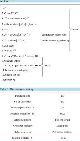
The pseudo code of the proposed algorithm is declared inAlgorithm 3.
4. Experimental Results
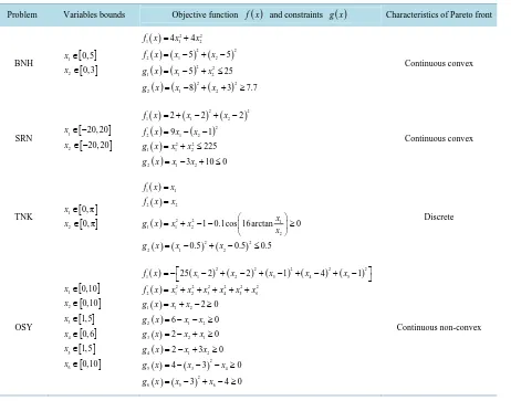
In order to validate the proposed approach and quantitatively compare its performance with other MOEAs, we present in this section comparison study for some benchmark test functions with distinct Pareto-optimal front, which was used in [28] [33]-[35]. The degree of difficulty of these problems varies from simple to difficult. Graphical presentation, of the experimental results and associated observations are presented in this section. Ta-ble 1 lists the parameter setting used in our algorithm for all runs andTable 2 lists the variable bounds, objec-tive functions and constraints for all these problems.
Algorithm 2. Operator for ε-approximate Pareto set.
{ }
{ }
1. : ,
2. 3. 4. 5. : 6. \ 7. 8. :
INPUT A x
if x A such that x x then A A
else
D x A x x A A x D end if Output A ε ′ ′ ∃ ∈ ′ = ′ ′ = ∈ ′ = ∪ ′
Algorithm 3. The proposed algorithm (pseudo code of the proposed al-gorithm). ( ) ( ) ( )
( )
( ) ( )(
)
( )(
( ) ( ))
{ } ( )(
( ) ( ))
0 0 0 0 1 1 1 02. Create ,
3. min
3. terminate , do
4. 1
5. , generate new search point
6. , update archive a
t
t t t
t t t
t
P R
A nondo ated P
while A t false
t t
P generate A P
A update A P
− − − = = = = + = =
{
( )}
( ) ( ) i i 1 lgorithm 3 7. 8. :8. , Dominted Pointes DS
9. Compute "Atom"
10. Comput Upper Bound , Lower Bound
11. new offspring.
12. Update NS set
t t Phase end while Output A A NS P Generate → → 2
13. NS
hase
[image:7.595.165.431.253.717.2]Output
Table 1. The parameter setting.
Population size 200
No. of Generation 200
Crossover probability Pc 0.9
Mutation probability Pm 0.02
Selection operator Roulette Wheel
Crossover operator Single point
Mutation operator Polynomial mutation
Table 2. Test benchmark problems used in our study.
Problem Variables bounds Objective function f x( ) and constraints g x( ) Characteristics of Pareto front
BNH [ ]
[ ] 1 2 0, 5 0, 3 x x ∈ ∈ ( ) ( ) ( ) ( ) ( ) ( ) ( ) ( ) ( ) 2 2
1 1 2
2 2
2 1 2
2 2
1 1 2
2 2
2 1 2
4 4
5 5
5 25
8 3 7.7
f x x x
f x x x
g x x x
g x x x
= +
= − + −
= − + ≤
= − + + ≥
Continuous convex
SRN [ ]
[ ] 1 2 20, 20 20, 20 x x ∈ − ∈ − ( ) ( ) ( ) ( ) ( ) ( ) ( ) 2 2
1 1 2
2
2 1 2
2 2
1 1 2
2 1 2
2 2 2
9 1
225
3 10 0
f x x x
f x x x g x x x g x x x
= + − + −
= − −
= + ≤
= − + ≤
Continuous convex
TNK [ ]
[ ] 1 2 0,π 0,π x x ∈ ∈ ( ) ( ) ( ) ( ) ( ) ( ) 1 1 2 2
2 2 1
1 1 2
2 2 2 2 1 2
1 0.1cos 16 arctan 0
0.5 0.5 0.5
f x x
f x x
x
g x x x
x
g x x x
= = = + − − ≥ = − + − ≤ Discrete OSY [ ] [ ] [ ] [ ] [ ] [ ] 1 2 3 4 5 6 0,10 0,10 1, 5 0, 6 1, 5 0,10 x x x x x x ∈ ∈ ∈ ∈ ∈ ∈ ( ) ( ) ( ) ( ) ( ) ( ) ( ) ( ) ( ) ( ) ( ) ( ) ( ) ( ) ( )
2 2 2 2 2
1 1 2 3 4 5
2 2 2 2 2 2
2 1 2 3 4 5 6
1 1 2
2 1 2
3 2 1
4 1 2
2
5 3 4
2
6 5 6
25 2 2 1 4 1
2 0
6 0
2 0
2 3 0
4 3 0
3 4 0
f x x x x x x
f x x x x x x x g x x x
g x x x
g x x x
g x x x
g x x x
g x x x
= − − + − + − + − + − = + + + + + = + − ≥ = − − ≥ = − + ≥ = − + ≥ = − − − ≥ = − + − ≥ Continuous non-convex
The BNH and the SRN problems are fairly simple in that the constraints may not introduce additional diffi-culty in finding the Pareto-optimal solutions as shown in Figure 4 and Figure 5. It was observed that all MOEAs methods performed equally well, and gave a dense sampling of solutions along the true Pareto-optimal curve.
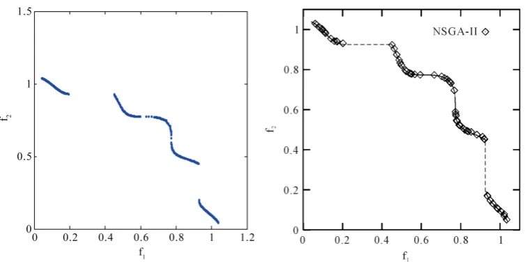
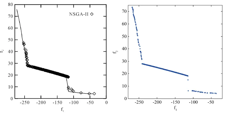
The TNK (Figure 6) and the OSY (Figure 7) are relatively difficult. The constraints in the TNK problem make the Pareto-optimal set discontinuous. The constraints in the TNK problem divide the Pareto-optimal set into five regions that can demand a proposed algorithm to maintain its sub-population at different intersections of the constraint boundaries. We compare our method with a reliable and efficient multiobjective genetic algo-rithm NSGA II. The results show that our method can be used efficiently for constrained MOP than NSGA-II. For the OSY problem, it can be seen that our approach gave a good sampling of points at the midsection of the curve and also found a lot of points at extreme ends of the curve. In the other hand NSGA-II did not give a good sampling of points at the extreme ends of Pareto curve.
Also, the proposed approach is applied to the problem was chosen from the engineering application, A welded beam design by Deb [36] and Two-Bar Truss [37] [38].
Welded Beam: A welded beam design is used by Deb [36], where a beam needs to be welded on another
beam and must carry a certain load F as shown inFigure 8.
Figure 4. Pareto optimal front of BNH problem using our approach.
Figure 5. Pareto optimal front of SRN problem using our approach.
[image:9.595.127.504.512.703.2]Figure 7. Pareto optimal front of OSY problem using our approach and NSGA-II.
Figure 8. Welded Beam design problem.
maximum rigidity (or minimum-end-deflection) are conflicting to each other, which leads to Pareto-optimal so-lutions. In the following, the mathematical formulations of the two-objective optimization problem of minimiz-ing cost and the end deflection are presented:
( )
(
)
( )
( )
( )
( )
( )
( )
( )
( )
[
]
[
]
( ) ( )
(
(
)
)
2 1
2 2
1 2
3 4
2 2 2 2
Min 1.10471 0.04811 14
Min 2.1952
s.t.
13600 0, 30000 0
0, 6000 0
, 0.125, 5 , 0.1,10
where
0.25
c
f x h l tb l
f x t b
g x r x g x x
g x b h g x P x
h b l t
l l h l
σ
τ τ τ τ τ
= + +
=
= − ≥ = − ≥
= − ≥ = − ≥
∈ ∈
′ ′′ ′ ′′
= + + + +
(
)
(
(
)
)
(
)
(
)
(
)
2 2
2 2
2
3
6000 2
6000 14 0.5 0.25
504000
2 2 12 0.25
64746.022 1 0.0282346 c
hl
l l h l
t b
hl l h t
P t tb
τ
τ σ
′ =
+ + +
′′ = =
+ +
= −
Figure 9. Pareto optimal front of welded beam using our ap-proach.
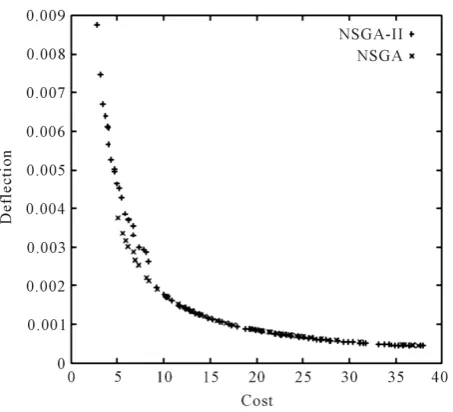
Figure 10. Pareto optimal front of welded beam using NSGA, NSGA-II.
distribution and spread.
Two-Bar Truss: Figure 11 illustrates the two-bar truss that is to be optimized [37]. This problem was
adapted from Kirsch [38]. It is comprised of two stationary pinned joints, A and B, where each one is connected to one of the two bars in the truss. The two bars are pinned where the join one another at joint C, and a 100 kN force acts directly downward at that point. The cross-sectional areas of the two bars are represented as x1 and x2,
the cross-sectional areas of trusses AC and BC respectively. Finally, y represents the perpendicular distance from the line AB that contains the two-pinned base joints to the connection of the bars where the force acts (joint C).
The problem has been modified into a two-objective problem in order to show the non-inferior Pareto set clearly in two dimensions. The stresses in AC and BC should not exceed “100,000 kPa” and the total volume of material should not exceed 0.1 m3. The reason the objective constraints have been imposed is that the Pareto set is asymptotic and extends from −∞ to ∞. As x1 and x2 go to zero, fvolume goes to zero and fstress BC, go to
infin-ity. As x1 and x2 go to infinity, fvolume goes to infinity and fstress AC, and fstress BC, go to zero. Hence, in order
[image:11.595.201.428.296.502.2](
)
(
)
(
)
(
)
0.5 0.5
2 2
1 2
0.5 2 ,
1
,
0.5 2 ,
2
1 2
Minimize 16 1
20 16 Minimize
subject to 0.1
100000
80 1
100000
1 3
, 0
volume
stress AC
volume
stress AC
stress BC
f x y x y
y f
yx
f f
y f
yx y
x x
= + + +
+ =
≤ ≤
+
= ≤
[image:12.595.218.411.86.257.2] [image:12.595.172.457.367.705.2]≤ ≤ >
Figure 12declares the Pareto optimal solution of the Two-Bar Truss. Obviously from the results, the pro-posed algorithm is able to maintain an almost uniform set of non-dominated solution points along the true Pare-to-optimal front. Figure 13 shows Pareto optimal front of Two-Bar Truss (MOGA Solution) [37] [38]. It is clear that the proposed algorithm outperformed the algorithm in [37] [38].
5. Conclusions
[image:12.595.228.397.375.507.2]Finding a good distribution of solutions near the Pareto optimal front in small computational time is a dream of multiobjective EAs researchers and practitioner. In this paper a new optimization algorithm was presented, and
Figure 11. Two-bar truss problem.
Figure 13. Pareto optimal front of two-bar truss (MOGA solution) [37] [38].
the proposed algorithm operates in two Phases. In the first one, multiobjective version of genetic algorithm is used as search engine in order to generate approximate true Pareto front. This algorithm is based on concept of co-evo- lution and repair algorithm. Also it maintains a finite-sized archive of nondominated solutions which gets iteratively updated in the presence of new solutions based on the concept of ε-dominance. Then in the second phase, rough set theory is adopted as local search engine in order to improve the spread of the solutions found so far. Our proposed approach keeps track of all the feasible solutions found during the optimization. The results, provided by the proposed algorithm for benchmark problems and engineering applications, are promis-ing when compared with exitpromis-ing well-known algorithms. Also, our results suggest that our algorithm is better applicable for solving real-world application problems.
For future work, we would like to apply our proposed algorithm for more complex real world application.
References
[1] Miettinen, K. (2002) Non-Linear Multiobjective Optimization. Kluwer Academic Publisher, Dordrecht.
[2] Mousa, A.A. (2013) A New Stopping and Evaluation Criteria for Linear Multiobjective Heuristic Algorithms. Journal of Global Research in Mathematical Archives, 1, 1-11.
[3] Cai, Q.S., Zhang, D.F., Wu, B. and Leung, S.C.H. (2013) A Novel Stock Fore-Casting Model Based on Fuzzy Time
Series and Genetic Algorithm. Procedia Computer Science, 18, 1155-1162.
http://dx.doi.org/10.1016/j.procs.2013.05.281
[4] Ni, H. and Wang, Y.Q. (2013) Stock Index Tracking by Pareto Efficient Genetic Algorithm. Applied Soft Computing,
13, 4519-4535. http://dx.doi.org/10.1016/j.asoc.2013.08.012
[5] Straßburg, J., Gonzàlez-Martel, C. and Alexandrov, V. (2012) Parallel Genetic Algorithms for Stock Market Trading Rules. Procedia Computer Science, 9, 1306-1313.
[6] Xue, X.-W., Yao, M., Wu, Z.H. and Yang, J.H. (2013) Genetic Ensemble of Extreme Learning Machine.
Neurocom-puting, Accepted Manuscript. (In Press)
[7] Yang, J.D., Xu, H. and Jia, P.F. (2013) Effective Search for Genetic-Based Machine Learning Systems via Estimation of Distribution Algorithms and Embedded Feature Reduction Techniques. Neurocomputing, 113, 105-121.
http://dx.doi.org/10.1016/j.neucom.2013.01.014
[8] Yang, H.M., Yi, J., Zhao, J.H. and Dong, Z.Y. (2013) Extreme Learning Machine Based Genetic Algorithm and Its Application in Power System Economic Dispatch. Neurocomputing, 102, 154-162.
http://dx.doi.org/10.1016/j.neucom.2011.12.054
[9] Osman, M.S., Abo-Sinna, M.A. and Mousa, A.A. (2005) A Solution to the Optimal Power Flow Using Genetic
Algo-rithm. Journal of Applied Mathematics & Computation (AMC), 155, 391-405.
[10] Osman, M.S., Abo-Sinna, M.A. and Mousa, A.A. (2009) Epsilon-Dominance Based Multiobjective Genetic Algorithm for Economic Emission Load Dispatch Optimization Problem. Electric Power Systems Research, 79, 1561-1567.
http://dx.doi.org/10.1016/j.epsr.2009.06.003
Power Flow Problem under Fuzziness. Journal of Natural Sciences and Mathematics, 6, 179-199. [13] Deb, K. (2001) Multiobjective Optimization Using Evolutionary Algorithms. Wiley, Chichester.
[14] Schaffer, J.D. (1985) Multiple Objective Optimization with Vector Evaluated Genetic Algorithms. In: Grefenstette, J.J.,
et al., Eds., Genetic Algorithms and Their Applications, Proceedings of the 1st International Conference on Genetic Algorithms, Lawrence Erlbaum, Mahwah, 93-100.
[15] Horn, J., Nafpliotis, N. and Goldberg, D.E. (1994) A Niched Pareto Genetic Algorithm for Multiobjective Optimiza-tion. In: Grefenstette, J.J., et al., Eds., IEEE World Congress on Computational Intelligence, Proceedings of the 1st IEEE Conference on Evolutionary Computation, IEEE Press, Piscataway, 82-87.
http://dx.doi.org/10.1109/ICEC.1994.350037
[16] Srinivas, N. and Deb, K. (1999) Multiobjective Optimization Using Nondominated Sorting in Genetic Algorithms.
Evolutionary Computation, 2, 221-248. http://dx.doi.org/10.1162/evco.1994.2.3.221
[17] Deb, K., Agrawal, S., Pratab, A. and Meyarivan, T. (2000) A Fast Elitist Non-Dominated Sorting Genetic Algorithms for Multiobjective Optimization: NSGA II, KanGAL Report 200001. Indian Institute of Technology, Kanpur. [18] Zitzler, E. and Thiele, L. (1998) Multiobjective Optimization Using Evolutionary Algorithms—A Comparative Case
Study. In: Eiben, A.E., Back, T., Schoenauer, M. and Schwefel, H.P., Eds., 5th International Conference on Parallel Problem Solving from Nature (PPSN-V), Springer, Berlin, 292-301. http://dx.doi.org/10.1007/BFb0056872
[19] Zitzler, E., Laumanns, M. and Thiele, L. (2001) SPEA2: Improving the Strength Pareto Evolutionary Algorithm for Multiobjective Optimization. Evolutionary Methods for Design, Optimization and Control with Applications to Indus-trial Problems, EUROGEN 2001, Athens, 19-21 September 2001, 1-21.
[20] Knowles, J.D. and Corne, D.W. (1999) The Pareto Archived Evolution Strategy: A New Baseline Algorithm for Mul-tiobjective Optimization. In: Proceedings of the 1999 Congress on Evolutionary Computation, IEEE Press, Piscataway, 98-105.
[21] Knowles, J.D. and Corne, D.W. (2000) M-PAES: A Memetic Algorithm for Multiobjective Optimization. In: Pro-ceedings of the 2000 Congress on Evolutionary Computation, IEEE Press, Piscataway, 325-332.
[22] Jimenez, F. and Verdegay, J.L. (1998) Constrained Multiobjective Optimization by Evolutionary Algorithm. Proceed-ing of the International ICSC Symposition on EngineerProceed-ing of Intelligent Systems (EIS’98), 266-271.
[23] Michalewiz, Z. (1996) Genetic Algorithms + Data Structures = Evolution Programs. 3rd Edition, Springer-Verlag, Berlin.
[24] Michalewicz, Z. and Schoenauer, M. (1996) Evolutionary Algorithms for Constrained Parameter Optimization Prob-lems. Evolutionary Computation, 4, 1-32.
[25] EL-Sawy, A.A., Hussein, M.A., Zaki, E.S.M. and Mousa, A.A. (2014) An Introduction to Genetic Algorithms: A Sur-vey A Practical Issues. International Journal of Scientific & Engineering Research, 5, 252-262.
[26] Fonseca, C.M. and Fleming, P.J. (1998) Multiobjective Optimization and Multiple Constraint Handling with Evolutio-nary Algorithms: Part I: A Unified Formulation. IEEE Transactions on Systems and Cybernetics. Part A: Systems and Humans, 28, 26-37. http://dx.doi.org/10.1109/3468.650319
[27] Harada, K., Sakuma, J., Isao, O. and Kobayashi, S. (2007) Constraint-Handling Method for Multi-Objective Function Optimization: Pareto Descent Repair Operator. Proceedings of the 4th International Conference on Evolutionary Mul-ticriterion Optimization, Matsushima, 5-8 March 2007, 156-170.
[28] Osman, M.S., Abo-Sinna, M.A. and Mousa, A.A. (2006) IT-CEMOP: An Iterative Co-Evolutionary Algorithm for
Multiobjective Optimization Problem with Nonlinear Constraints. Journal of Applied Mathematics & Computation,
183, 373-389. http://dx.doi.org/10.1016/j.amc.2006.05.095
[29] Hernández-Díaz, A.G., Santana-Quintero, L.V., Coello Coello, C.A., Caballero, R. and Molina, J. (2008) Improving Multi-Objective Evolutionary Algorithms by Using Rough Sets. In: Ligeza, A., Reich, S., Schaefer, R. and Cotta, C., Eds., Knowledge-Driven Computing: Knowledge Engineering and Intelligent Computations, Studies in Computational Intelligence, Vol. 102, Springer-Verlag, Berlin, 81-98.
[30] Laumanns, M., Thiele, L., Deb, K. and Zitzler, E. (2002) Archiving with Guaranteed Convergence and Diversity in Multi-Objective Optimization. GECCO 2002: Proceedings of the Genetic and Evolutionary Computation Conference, Morgan Kaufmann Publishers, New York, 439-447.
[31] Osman, M.S., Abo-Sinna, M.A. and Mousa, A.A. (2005) An Effective Genetic Algorithm Approach to Multiobjective Resource Allocation Problems (MORAPs). Journal of Applied Mathematics & Computation, 163, 755-768.
http://dx.doi.org/10.1016/j.amc.2003.10.057
[32] Murata, T., Ishibuchi, H. and Tanaka, H. (1996) Multiobjective Genetic Algorithm and Its Application to Flowshop Scheduling. Computers and Industrial Engineering, 30, 957-968.
[33] Binh, T.T. and Korn, U. (1997) MOBES: A Multi-Objective Evolution Strategy for Constrained Optimization Prob-lems. Proceeding of the 3rd International Conference on Genetic Algorithm MENDEL, Brno, 176-182.
[34] Osyczka, A. and Kundu, S. (1995) A New Method to Solve Generalized Multicriteria Optimization Problems Using the Simple Genetic Algorithm. Structural Optimization, 10, 94-99.
[35] Tanaka, M., Watanabe, H., Furukawa, Y. and Tanino, T. (1995) GA-Based Decision Support System for Multi-Criteria Optimization. Proceeding of the International Conference on Systems, Man and Cybernetics, 2, 1556-1561.
[36] Deb, K., Pratap, A. and Moitra, S. (2000) Mechanical Component Design for Multiple Objectives Using Elitist Non- Dominated Sorting GA. Kangal Report No. 200002.
currently publishing more than 200 open access, online, peer-reviewed journals covering a wide range of academic disciplines. SCIRP serves the worldwide academic communities and contributes to the progress and application of science with its publication.
![Figure 2. Decision variable space (left) and objective function space (right) [29].](https://thumb-us.123doks.com/thumbv2/123dok_us/8075203.780756/3.595.142.483.398.512/figure-decision-variable-space-objective-function-space-right.webp)


![Figure 13. Pareto optimal front of two-bar truss (MOGA solution) [37] [38].](https://thumb-us.123doks.com/thumbv2/123dok_us/8075203.780756/13.595.173.457.84.243/figure-pareto-optimal-bar-truss-moga-solution.webp)
