Model-Based Predictive Adaptive Delta Modulation
Anas Al-korj and Sandor M Veres
*Mechanical Engineering, University of Southampton, Highfield, Southampton, SO17 1BJ, UK (emails: [email protected], [email protected])
Abstract: This paper presents a new technique in digital communications that is called model-based-predictive adaptive-delta-modulation (MBP-ADM). MBP-ADM uses system identification tools to identify a model of the signal which is used for prediction. Prediction helps the system to respond adaptively to a varying input signal in order to achieve improved performance. The results show a substantial improvement in the signal to noise ratio (SNR) of MBP-ADM’s compared to the ‘classical adaptive’ and ‘non-adaptive’ delta modulators.
1. INTRODUCTION
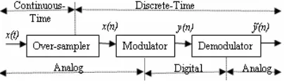
[image:1.595.44.246.407.467.2]Delta modulation (DM) performs high resolution analog to digital conversion (ADC) using low complexity components. The main steps in DM (or any other differential-based digital modulator) are shown in Fig. 1.
Fig. 1. The main steps in Delta Modulation
The analog signal x(t) is sampled at a rate higher than the Nyquist rate in the over-sampler block in Fig. 1. Each sample x(n) is converted into digital values y(n) in the modulator. Delta modulation is a predictive quantizing system and is essentially a one-digit differential pulse code modulation (Abate, 1967). In linear DM, the predicted value is a linear function of the past values of the quantized signal. In adaptive DM (ADM), the predicted value of the input signal is a nonlinear function of the past values of the quantized signal. To get an optimum performance in DM, it is required to introduce nonlinear prediction to force the system to respond adaptively to any changes in the slope of the input signal. Optimal performance is achieved by extending the dynamic range over which DM operates (Abate, 1967). Another modified and important version of DM is called the Sigma-Delta Modulator (SDM). The SDM is well-known and was developed for the purpose of coding DC signals, and for further simplifying the demodulator. Adaptive SDM (ASDM) is also a well-established area in the ADC field (see for example (Aldajani and Sayed, 2001; Zierhofer, 2000; Aziz, et al., 1996). Several adaptation techniques for DM and SDM have been investigated over the last five decades (Abate, 1967; Aldajani and Sayed, 2001; Zierhofer, 2000; Aziz, et
al., 1996).
The main objective of the new method of model-based predictive adaptive delta modulation (MBP-ADM), which is introduced in this paper, is to employ the advantages of Model-based predictive control (MPC) in the field of digital communications. This approach has been developed and implemented as an alternative to the existing ‘classical’ capacitor-based mechanism for one-step-ahead prediction in classical DM. MBP-ADM applies k-step ahead model-based predictive control as an alternative to the one-step ahead classical prediction, which is often implemented by simple integrators using capacitors. Some of the on-line implementation issues of MBP-ADM are also addressed in the paper, by studying methods for finding the optimum selection of parameters to minimize the error to noise ratio and the processing time. It will be shown that this union between long-range-MPC techniques and digital communications helps to overcome many problems in digital differential communication systems.
In this paper, techniques of k-step-ahead model-based prediction are introduced to help in resolving the following three problems:
• To overcome the problems associated with the classical integration which is used as the 1-step-ahead predictor.
• To overcome the undesirable effects of the variations in the uncontrollable variables, namely, the amplitude and the frequency of the input signal. This means that MBP-ADM generates a minimum value of the sum of all noises: the slope overload noise, and granular noise. This feature is inherited from the fact that the integrator is not needed anymore.
Further advantages of direct long-range prediction includes: better detection of the synchronization signals, which are usually embedded within the data stream, (when dealing with command signals for example), and handling constraints which usually come from the electrical characteristics of the participating components. Section II illustrates both the classical adaptive and non-adaptive DM. Section III introduces MBP-ADM. An example and the results are in Section IV.
[image:2.595.304.554.69.217.2]2. CLASSICAL ‘DELTA’ & ‘ADAPTIVE DELTA’ MODULATIONS
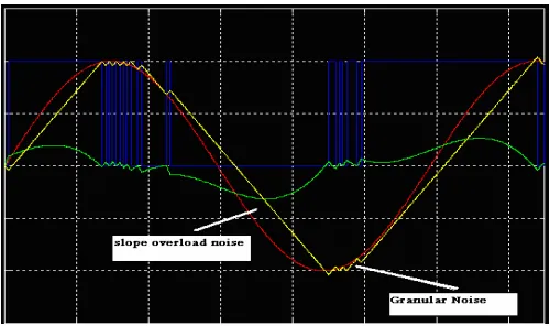
Fig. 3, Types of Noise in DM: Slope-overload noise, and Granular noise.
Delta modulation, and all the issues associated with the noise and performance have been extensively studied in (Steele, 1975). A block diagram of DM is shown in Fig. 2.
The need to minimize both of these results in conflicting requirements when selecting the step size or the integrator gain. One solution is to select the step size to minimize the sum of the mean square values of these two distortions (Steele, 1975).
[image:2.595.44.284.283.375.2]The complexity of the problem comes from the fact that, increasing the step for the sake of reducing the slope overload noise will increase the granular noise and vice versa, as shown in Fig. 3 and Fig. 4.
Fig. 2, Implementation of classical DM
The key step for an effective use of delta modulation is the intelligent choice of the two parameters, the ‘step size’ and the ‘sampling period’.
[image:2.595.308.553.369.470.2]These must be chosen so that the signal cannot possibly change too fast for the steps to follow accurately. If the steps cannot follow changes in the signal, the situation is known as overloading. Since the signal has a definable upper-frequency cut-off, we usually know the fastest rate at which this can change. However, to account for the fastest possible change in the signal, the sampling frequency and/or the step size must be increased. Increasing the sampling frequency will result in the delta-modulated (coded) waveform requiring a larger bandwidth for transmission. On the other hand, increasing the step size increases the quantization error. That is, the step approximation to the function becomes poorer as the step size increases. This is most obvious during periods when the function is almost constant.
Fig. 4, Noise in DM vs. Integrator step size.
For a given system, and for each sampling period, there will be an optimum step value which should be determined. To further improve the performance, an adaptive delta modulation scheme (ADM) can be used. Several schemes have appeared over the last three decades. Most of these schemes are of a feedback type, where the digital code in the output is used to achieve the adaptation, see for example (Abate, 1967) and (Gregorian and Gord, 1983). Practically speaking, most of the ADM systems depend on monitoring the digital output data and try to adapt the step size depending on the incoming input signal as shown in Fig. 5.
The two main types of noise can be easily observed in Fig. 3: ‘slope overload noise’ and ‘granular noise’.
Fig. 5, Block diagram of a continuously variable slope [adaptive] DM
3. MBP-ADM SCHEME
[image:3.595.333.528.110.202.2]Signals sampled at the Nyquist rate or faster exhibit significant correlation between successive samples. In other words the average change in the amplitude between successive samples is relatively small. Consequently, an encoding scheme that exploits the redundancy in the samples will result in a lower bit rate for the source output. A relatively simple solution is to encode the differences between successive samples rather than the samples themselves. Since the differences between the samples are expected to be smaller than the actual sampled amplitudes, then fewer bits are required to represent the differences. The main structure of MBP-ADM will take the form shown in Fig. 7. An explanation of the main blocks in MBP-ADM is given in the following subsections.
Fig. 7, Structure of MBP-ADM scheme as compared with classical DM: The upper feedback loop represents classical delta DM, and the lower feed forward loop represents model-based predictive adaptive DM (MBP- ADM).
3.1. Model Identification
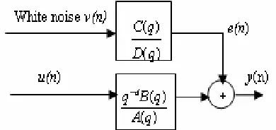
The general case of a linear input-output model for a single-input single-output system with single-input u, and output y, is shown in Fig. 8. Here u denotes the input, and A, B, C, and D,
are polynomials in time shift operator q. The noise is represented by v.
Figure 8, General linear model for a single output
A and B are given by:
(1) nB nB nA nA q b q b q b b q B q a q a q a q A − − − − − − + + + + = + + + + = ... ) ( ... 1 ) ( 2 2 1 1 0 2 2 1 1
Various model forms can be achieved as special cases of Fig. 8, (Ljung, 1994).
i) ARX: A(q) y(n) = B(q) u(n-d) + v(n)
ii) ARMAX: A(q) y(n) = B(q) u(n-d) + C(q) v(n)
iii) OE: y(n) = [B(q)/F(q)] u(n-d) + v(n)
iv) BJ: y(n)=[B(q)/F(q)] u(n-d)+[C(q)/D(q)] v(n)
When modelling time series there will be no input signal, and the general ARMAX model is reduced to the ARMA model structure (Veres and Wall, 2000; Ljung, 1994).
D(q) y(n) = C(q) v(n) (2)
Different model orders can be used for MBP-ADM. The effect of the model order will be investigated at a later stage. There are many available algorithms and packages for modelling, which can be used to identify the model. The System Identification Toolbox in MATLAB was used to perform the identification in this study.
3.2. k-steps-ahead model-based prediction
This is the core element in the MBP-ADM scheme. The predictor in this study substitutes the classical prediction method in both classical DM as well as in classical ADM. Traditionally, both DM and ADM use the integrator’s concepts and mechanisms with some form of automatic gain control (AGC), to get a predicted value of the tracked signal and then use a suitable speed (integrator’s gain) to reduce the tracking error. While in the proposed method of MBP-ADM, in order to predict the output over the prediction horizon, a k-step-ahead predictor is required.
A k-step-ahead prediction of the process output must be a function of all the data up to ‘n’, the future controller output sequence, some noise, and a model of the process k) (n ˆ + y $
[image:3.595.43.292.450.595.2]yˆ (n + k) = ƒ (u, ϕ,H$) (3)
Where ƒis a function and ϕ is a vector represents all the data up to ‘n’. Clearly, the k-step-ahead predictor will depend heavily on the model. In order to take the disturbances into account when predicting the output of the process, the disturbances must also be modelled. The model with a disturbance term v(n) which is given by:
( 1) ( ) ) ( ) ( ) ( 1 1 n e n u q A q B q n y d + −
= − − − (4)
The disturbance e(n) may in general be a sum of deterministic and stochastic disturbances. The k-step-ahead predicted output is given by:
( 1) ( )
) ( ) ( ) ( ˆ 1 1 k n e k n u q A q B q k n y d + + + + =
+ − −− (5)
The disturbances which can not be predicted exactly are modelled by: ) ( ) ( ) ( ) ( 1 1 n v q D q C n e − −
= (6)
Where e(k) is a signal which can be measured but cannot be predicted, and C and D are polynomials with degree and
. The predicted e(n) is given by:
C n D n ( ) ) ( ) ( ) ( ˆ 1 1 k n v q D q C k n
e + = − +
−
(7)
Where v(n+k) is a white noise sequence.
3.3. The quantizer and the digital sampler
This quantizer and the digital sampler block are exactly the same as in any classical delta or classical adaptive delta modulators, see (Steele, 1975).
4. IMPLEMENTATION AND RESULTS
In this section a comparison is made between the performance of the MBP-ADM scheme and the classical ADM. Both ADM and MBP-ADM were fully implemented and tested in MATLAB/SimulinkTM. Both systems were fully implemented in hardware circuits in laboratory.
4.1. ADM versus MBP-ADM
The methods were tested both on electronic hardware and in simulation. The results from the hardware testing are consistent with the results from the MATLAB/Simulink simulations. The signal is modelled using auto regressive moving average (ARMA) model. A robustified quadratic prediction error criterion is minimized off-line using an
iterative Gauss-Newton algorithm. A comprehensive investigation about the choice of model order for this application was made in (Al-korj, 1999). The identified 10th order ARMA model for signal presented above was D(q) y(n) = C(q) v(n) with:
D(q) = 1 - 1.733 q^-1 - 0.5182 q^-2 + 1.417 q^-3 + 1.526 q^-4 - 1.707 q^-5 - 0.8857 q^-6 + 0.8195 q^-7 + 0.1577 q^ -8 + 0.06576 q^-9 - 0.1327 q^-10,
and
C(q) = 1 - 1.09 q^-1 - 0.8757 q^-2 + 0.6268 q^-3 + 1.522 q^-4 - 0.8194 q^-5 - 0.7352 q^-6 + 0.3456 q^-7 + 0.1231 q^-8 + 0.0407 q^-9
The identified model was used to predict the tracking signal. This predicted tracking signal was compared with the actual signal, and the digital output sequence is formed. Then this digital sequence was sampled with the same sampling rate to generate (off-line) the model-based predictive adaptive delta modulated signal. The adaptation was done of-line and digitally using hybrid circuitries.
For both cases of ADM and MBP-ADM, performance can be measured by the sum of the error square divided by the maximum value of the signal and multiplied by 100 to give a percentage.
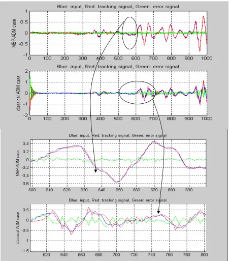
After applying the same signal to both systems, and using 10-step-ahead prediction schemes, the result are as follows:
• The error to signal percentage for the classical case is equal to 0.6 % of the signal in the above example.
• The error to signal percentage for the MBP-ADM case is equal to 0.16% of the same signal and in exactly the same conditions.
Therefore, the improvement for k = 10 in our steps-ahead prediction was four times better than in the classical case: 0.6 / 0.16
≅
4 times improvement.When working with only one-step-ahead prediction, the model based prediction error is 0.021616%, i.e. the improvement in MBP-ADM over the classical method (based on only one-step-ahead) is as follows: 0.6/0.021616
≅
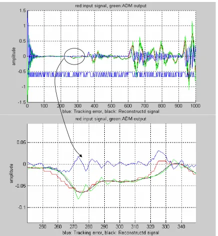
27 times improvement. Figure 9 (in page 6), illustrates the error differences in both ADM and MBP-ADM.5. CONCLUSIONS
IEEE Journal of Solid-State Circuits, Vol. SC-18, No. 6, 5. REFERENCES
pp 692-700. Abate, J. E., (1967), Linear and adaptive Delta modulation,
Ljung, L. (1994). System Identification – Theory for the Proceedings of the IEEE, Vol. 55, No. 3, pp. 298-308.
user. Englewood Cliffs: Prentice Hall. Morari, M. and Aldajani, M.A. and A.H. Sayed (2001). Stability and
N.L. Ricker, (1985). Model Predictive Control Toolbox performance analysis of an adaptive Sigma Delta mod-
for use with MATLAB, The MathWorks Inc., ulators, IEEE Transactions on circuits and systems-II:
http://www.mathworks.com/products/mpc Analog and digital signal processing, Vol. 48, No. 3,
Proakis, J.G. (1983). Digital Communication. McGraw Hill, pp. 233-244.
USA. Al-korj, A. (1999). Model-Based Predictive Delta Mod-
Steele, R. (1975). Delta Modulation Systems, Pentech Press, ulation, MSc dissertation, University of Sheffield, UK.
London. Aziz, P.M., H.V. Sorensen, and J. V. D. Spiegel (1996). An
Veres S.M. and D.S. Wall, Synergy and Duality of Iden- overview of Sigma-Delta converters: How a 1-bit ADC
tification and Control. Taylor & Francis, 2000. achieves more than 16-bits resolution, IEEE Signal pro-
Zierhofer, C.M., (2000). Adaptive Sigma-Delta modulation with one-bit quantization, IEEE Transactions on circuits and systems-II: Analog and digital signal processing, Vol. 47, No. 5, pp.408-415.
[image:5.595.83.518.274.746.2]cessing magazine, Vol. 13, No. 1, pp. 61-84. Gregorian, R. and J.G. Gord, (1983). A Continuously variable slope adaptive delta modulation codec system,