Instance Segmentation of Point Clouds using Deep Learning

(1)

Instance Segmentation of Point

Clouds using Deep Learning

Master in Innovation and Research in Informatics (MIRI)

Facultat d’Informatica de Barcelona (FIB) Universitat Polit`ecnica de Catalunya

Author:

Gerardo Francisco P´erez Layedra

Director:

Javier Ruiz Hidalgo

Ponent:

Lluis Belanche Mu˜noz

Data Mining and Business Intelligence Barcelona, Spring Semester, 2018

(2)

I am most grateful with my family, without their support I could not accomplish any of the goals I did, they are my inspiration and the source of my strength. This work is for them.

To my teachers, every single one of you has left technical and personal knowledge that I will use in the best possible way.

(3)

Abstract

Point cloud is an efficient way to represent 3D objects, creating complex scenes out of them. With technology advances like 3D scan cameras, this has become a popular way for 3D mapping, mesh creation, object surface analyses and what concerns us, the creation of vast datasets.

Recent advances in deep learning networks had provided efficient way to process this data, like PointNet and PointNet++ a novel 3D deep learning network that segments 3D point clouds in semantically meaningful classes, but at the time of the creation of the present work, there is no procedure to instantiate objects from a 3D point cloud scene. The main objective of this investigation work is to implement a deep network architecture to segment and instantiate objects on 3D point clouds using PointNet, as a baseline. This investigation work will extend the PointNet network, with emphasis on the segmentation approach, and then predict a value that represents the instance of the different objects of the 3D point cloud.

(4)

(5)

Table Index

4.1 Hardware details . . . 23

4.2 Total count of objects in Stanford Dataset . . . 24

4.3 Hyperparameter values and configurations run for all experiments, several other cases were tested, the values presented in this table are the most accurate ones, based on accuracy and loss onto the test, validation and test executions. . . 28

5.1 Evaluation of classification for scenario 1 . . . 31

5.5 Results for overall accuracy for all experiments . . . 37

1 Evaluation of classification for scenario 1 . . . 48

(10)

(11)

List of Figures

1.1 Instantiation segmentation of image . . . 2

2.1 Point cloud representation of Highway[7] . . . 4

2.2 McCulloch and Pitts artificial neuron . . . 5

2.3 Artificial neuron (perceptron) . . . 6

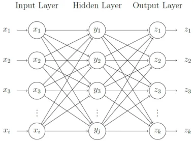
2.4 Multilayer perceptron representation with three layers, with i input layers, j artificial neurons, and k neurons in the output layer. . . 6

2.5 Step activation function for MCP . . . 7

2.6 Sigmoidal activation functions. . . 9

2.7 Different opuputs for weight initialization to zero (a), standard devi-ation generdevi-ation (b) and normal devidevi-ation (c). . . 10

2.8 Gradient descent . . . 11

2.9 Learning rate values exemplified, with a) large and b) small values . . 12

2.10 Definition of Intersection Over the union . . . 13

3.1 Pixelwise example architecture fromPixelwise Instance Segmentation with a Dynamically Instantiated Network[24] . . . 16

3.2 The input point cloud is projected into multiple virtual camera views, generating virtual images, these images are preocessed by an CNN for semantic segmentation and the output prediction scores from all views are fused into a single prediction for each point. . . 17

(12)

3.3 Use of PointNet. It is a unified architecture that learns both global and local point features, providing a simple, efficient and effective

approach for a number of 3D recognition tasks . . . 18

3.4 PointNet Architecture . . . 19

4.1 Dataflow computational graph[29] . . . 21

4.2 Stanford Dataset Sample - Area 2 . . . 23

4.3 Areas object balance count . . . 25

4.4 Distribution of points from the centroid of the object . . . 26

4.5 Histogram with the distribution of the 13 D classes in the dataset . . 27

4.6 Coloured point cloud with its RGB values. Each distance had been normalized in the range [0,12], being the center 0 and the borders 12 27 5.1 Results for Scenario 1, contains a) the train results, b) validation set, c) evaluation of each epoch, d) train results. For a), b), and c) the x coordinates represent the number of epochs, d) contains the number of models used in test. . . 30

5.2 Ground truth (a) and Prediction (b) values for scenario 1 . . . 31

5.3 Results for Scenario 2, contains a) the train results, b) validation set, c) evaluation of each epoch, d) train results. For a), b), and c) the x coordinates represent the number of epochs, d) contains the number of models used in test. . . 32

(13)

1 Tensorboard output when the value to predict is the euclidean dis-tance D . . . 47 2 Tensorboard output when the value of R had been replaced with L . 49 3 Tensorboard output when the value of L had been added to the

net-work input . . . 51 4 Tensorboard output when the value of Land customRGB had been

(14)

Introduction

This chapter describes the motivation and objectives to be accomplish in this inves-tigation, it serves as a gentle introduction into what the research is to be about and what are the expects results, also giving brief technical notions to be expanded in further chapters.

1.1 Motivation

Advances in machine and deep learning techniques are present in a variety of daily life aspects, from ”simple” games like Google Quickdraw[1] to Image to Im-age generation[2], it is obvious that we are moving to an data driven era, where techniques that can identify patters from high dimensional data in every field of investigation are becoming more and more important.

Object segmentation consist in the division of an initial image into smaller, more easy to handle pieces, giving a better representation of the most prominent aspects of the image, classifying them and making it easier to analyze. Instantiation con-tinues this classification, identifying different objects that belong to the same class, expanding even more the information that can be extracted from an image.

Previous approaches onto 2D instantiation segmentation had proven to be accurate[3] as shown on figure 1.1.

(15)

Figure 1.1: Instantiation segmentation of image

When it comes to 3D objects, PointNet[4] provides an efficient and accurate framework for segmentation of point clouds, but there is no method currently de-veloped for point cloud instantiation, creating a necessity for it.

1.2 Objectives

The main objective of this investigation, is to create and evaluate a deep learning framework for instance segmentation using unordered point clouds as input, and thus achieve object wise recognition in a 3D environment, parting from the cases that a group of points in the cloud could be part of an object having the same semantic class or could not be part of the same object but could have the same semantic class.

(16)

Fundamentals

The chapter is intended to be an introduction for the unfamiliar reader, contains the basic knowledge of all the concepts, technologies and techniques applied. It starts with technical topics, explaining the basis of what a point cloud is, then introducing the basics about deep learning, a description of PointNet, a novel point cloud deep learning processing architecture

2.1 Point Cloud Representation

Point cloud contains data that represents the external surface of an object into a three dimensional structure system that is given into the X, Y, Z coordinates and some other data, like color or textures. In early stages, for a correct 3D mesh cre-ation, this data initially needed preprocesing; but with better techniques to represent the objects directly from the point clouds[5], the consumption of computational re-sources and time, had been reduced, popularizing the use of point clouds in data analysis and 3D modeling.

These data are created through 3D scanners, in recent years with new and accessible technologies in the market (like Microsoft’s Kinect, Orbbec Astra, Intel RealSense, etc.) anyone with fairly decent computational resources could scan a 3D environ-ment and create its own point cloud dataset. There exist even specialized software like PointCab[6] that can render these data based on drone video input data. To further increase the use of this technology, new miniature scan devices integrated for example into mobile devices, such as the iPhone X’s TrueDepth camera, had allowed new possibilities.

Data clouds of points are used to create visual representation of surfaces for quality inspection, animation rendering, medical imaging, data analysis of 3D objects, as it is a trusted and easy way to manipulate 3D surface data, figure 2.1 contains a representation of how this data collection is visualized.

(17)

Figure 2.1: Point cloud representation of Highway[7]

2.2 Deep Learning

Deep learning[8] is a fast growing technique for automated learning nowadays, it is composed of mathematical models that allow representations of data to be learned from them, through the use of multiple processing layers, that transforms the input representation at each level into a higher, more abstract level, so with enough of this levels, complex models can be learned. The inspiration for deep learning, came from how the neurons of the visual cortex works, these neurons react different to each other, depending on the scenario which they are exposed. The combinations of these neurons can be used to represent very complex scenarios.

Deep learning most common use are for supervised learning. For example in classifi-cation tasks, the higher layers are in change of amplify aspects that are relevant, and suppress the irrelevant ones, often through the weighted connection to previously activated layer, so in each one of them the data will be more and more specialized. The beauty of this is that the weighted connections are not hand-designed, but rather learned through an automated learning process. A technique which allows for the models to improve with experience and data given[9]

Today these models are widespread in nearly every major topic of research and inves-tigation like speech and visual recognition[10], medicine[11], stock market forecast[12], etc., resulting in an improvement in their performance and state of the art.

(18)

2.2.1 Artificial Neural Networks

Artificial neural networks are the basis of deep learning, as the name may imply, they are inspired by the neurons of the human brain, that working as a whole, could be seen as a biological network. In this field, the learning occurs when the synapses of the neurons activates or inhibits the electrical impulses sent between them, so the influence of one neuron changes.

Their artificial counterpart was first proposed in 1943 by Warren McCulloch and Walter Pitts, this so called MCP (McCulloch-Pitts-Neuron) as illustrated in figure 2.2 in this definition, each neuron is a binary device, with a fixed threshold and equal weight for all the excitatory input; this concept was a cornerstone of future investigations, but had a great disadvantage, because their definition of weights and threshold are static, so it had no learning capabilities.

Figure 2.2: McCulloch and Pitts artificial neuron

To overcome this limitation in 1959 the first computational, trainable neural networks were developed by Rosenblatt[13], and continued with further works by Widrow and Hoff[14] and Widrow and Stearns[15]. Rosenblatt initially proposed the concept of aPerceptron which was a neural network with two layers of computational nodes and a single layer of interconnections, this concept was limited to the solution of linear problems, but represents the basis of what we are using in modern days. The perceptron can be defined as

f(x) =

(

1 if w.x >0 0 otherwise

where w is a vector of real weights, w.x the scalar product and t the threshold value.

In a brief description, the neuron (perceptron) a local computing device that gets a vector as an input, then combines it with its local weights that can amplify or decrease the original input signal, add his values together with local information, pass them through an activation function to get a desired scalar result. These can be seen in

(19)

Figure 2.3: Artificial neuron (perceptron)

2.2.2 Multilayer Perceptron

It is in 1974 with the work of Werbos[16] that the concept ofMultilayer Perceptron

appears, expanding the artificial neural networks to nonlinear calculations. These MLP consist on multiple fully connected layers, minimum three as detailed in figure 2.4 of nodes (neurons), each one contains a nonlinear activation function and are trained via backpropagation, by comparing the amount of error in each output to the expected value, and then updating the weights after each batch of data is processed, so the error is calculated in the output layers and then redistributed to the previous layers. Gradient descent optimization algorithm makes extensive use of backpropagation, finding and adjusting new values up until the local minima is found.

Figure 2.4: Multilayer perceptron representation with three layers, with i input layers, j artificial neurons, and k neurons in the output layer.

(20)

2.2.3 Activation Functions

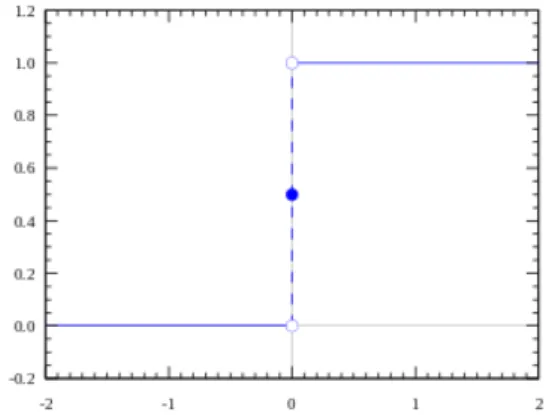
In the learning process of a neural network, it is important to always take into account that not all data are equally useful, even if a scrupulous data cleaning and preparation some of it could be considered just as noise, so a method that allow to exclude these noise is needed, the activation function inside a neural network accomplishes this objective, it is what determines whether an outside connection should consider the neuron as activated if the value produced by the neuron Y is above certain value, or not otherwise. Figure 2.5 represents the activation function initially proposed by MCP neurons.

Figure 2.5: Step activation function for MCP

This activation function is limited to binary classification values, so more complex tasks where intermediate activation values are needed are impossible to obtain, in this case a non linear activation function can give the desired output. The most widely used non linear activation functions are the sigmoidal ones, that takes on values into the [0,1] range, being the most negatives ones represented by 0 and the highest ones as 1. Sigmoidal activation functions are defined as:

σ(x) = 1 1 +e−x

However, sigmoidal functions are also not suited for every kind of data, to deal woth some of the limitations of sigmoidal activation function there is thetanh non linearity activation function, is actually just a scaled sigmoid neuron which maps the input to a number in the range [-1,1], which actually solves, allowing far more flexibility. It is expressed as

tanh(x) = 2σ(2x)−1

Also there is ReLU activation functions, that gives an output x if x is positive, and 0 otherwise, this definition may sound similar to the linear function one, but

(21)

the ReLU function definition, stated above, is not linear, and their combinations are also non linear, providing a good aproximator.

f(x) =max(0, x)

ReLU functions solve one important issue of sigmoidal and tanh functions, they deal with the sparsity problem of the activation very well, as not all of the neurons will be activated at the same time, just the ones that are in the positive side of

x, making the network lighter. But this has a drawback, as the activation in the negative side are never fired, the weights are not updated during backpropagation, causing a problem called”dead neurons” making a big part of the network passive. There are several ways to deal with the dead neurons problem, one is the Leaky ReLU function that allows negative values, which reduces the number of dead neurons. Another one isParameterised ReLUmuch similar lo Leaky ReLU, but the α value is also trainable, for a faster, more optimum convergence. Leaky and Parameterised ReLU are defined as:

f(x) =

(

x x≥0

αx x <0 Where α is the threshold of the negative values allowed.

Softmax activation function is generalization of the logistic functions, that deal better with clasification problems than Sigmoid and ReLU activation functions. It works similar to Sigmoid function, but also normalizing the values of each unit in the range [0,1], so the total sum of outputs is equal to 1, that way, Softmax is equivalent to a categorical probability distribution, giving the probability on which each of these cases are true. The mathematical definition of Softmax is:

σ(z)j =

ez PK

k=1ezj

Where z is a vector of the inputs to the output layer.

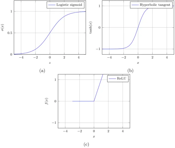
Figure 2.6 contains a graphical description of the behaviour of these activation functions.

(22)

−4 −2 0 2 4 0 0.5 1 z σ ( x ) Logistic sigmoid (a) −4 −2 0 2 4 −1 0 1 x tanh( x ) Hyperbolic tangent (b) −4 −2 0 2 4 −1 0 1 x f ( x ) ReLU (c)

Figure 2.6: Graphical representations of the (a) Sigmoid activation function, (b) Hyperbolic tangent tanh(x) and (c) Rectified Linear Unit. ( z )

2.2.4 Cross Entropy

Cross entropy is the measurement between two probability distributions, mathemat-ically is defined as:

H(p, q) =−X i

pi(log(qi))

The basic idea for the classifier to be consider as acceptable, is to find the correct value of the parameters, giving high distances for those classes that incorrectly labeled, and low ones for those correctly labeled, in other words, minimize the average of the cross entropy, this is called the loss function, and its values are what makes the classifier acts as expected.

(23)

(a) Initial Weights Set to Zero (b) Initial Weights drawn N(0, σ= 0.4)

(c) Initial Weights N(0, σ∼p2/nj)

Figure 2.7: Different opuputs for weight initialization to zero (a), standard deviation generation (b) and normal deviation (c).

2.2.5 Weight Initialization

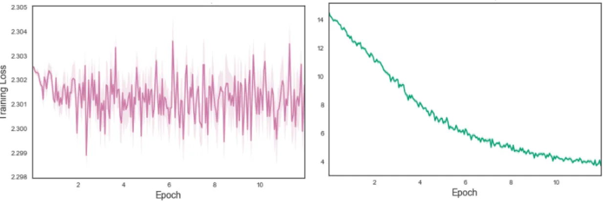
With the broad aspects that deep learning methods has to deal with, selecting an accurate weight initialization method is not a light subject, weight initialization se-lection has an important impact on the final convergence rate and accuracy of the model, even recent research’s[17] dedicate a lot of effort into this endeavour. Image 2.7 represents the different results obtained for a 10 batch rolling average of the loss of the train of a convolutional neural network with different activation function approaches.

For example, Xavier weight initialization, creates the weights from a distribution with zero mean and a specific variance, given by

V ar(W) = 1

(24)

w[0]

w[1]

w[2]

w[3]

w[4]

Figure 2.8: Gradient descent

on which W is the initialization distribution for the neuron, nin in the neurons

in the networks.

2.2.6 Backpropagation

Backpropagation is one of the key aspects for learning in deep neural networks. In backpropagation, the error contribution of each neuron after a batch of data is pro-cessed is calculated, and then propagated backwards thought all the network. The objective of this technique, is to minimize the loss function applied, by tunning its weights, so for example in a multilayered network, it will learn the correct inter-nal representations for any given model. This minimization is done by taking the derivatives of the squared error function with respect to the weights of the proposed model and following the direction of the gradient on which it reduces, this is called the gradient descent method, which is graphically explained in figure 2.8.

Gradient descent method could compute the gradient values for the entire dataset, but as the operations are computationally costly, there are several approaches that deals with this, the first one isStochastic Gradient descent, that uses a few training examples to do the calculations of the gradients, generally this method leads very abrupt changes when outliers are found. Another method is Mini Batch Gradient Descent, which consists on taking smaller pieces of the complete dataset, and process them, there are several considerations into the sizes and performance of the Mini Batch technique[18], however this topics are too abroad to discuss in this investiga-tion work.

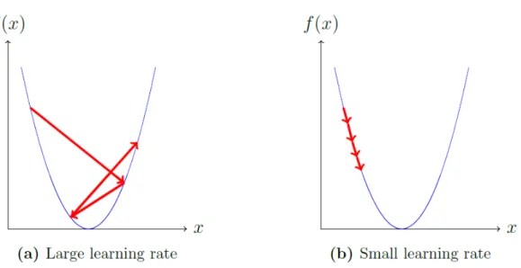
An important aspect to take into account in gradient descent is the learning rate, that is the value on which each weights update overtime, if the learning rate is too big, the values might never converge, and if there is too small, the problem could take a ling time to get to the optimum result. This scenario is shown in 2.9.

(25)

Figure 2.9: Learning rate values exemplified, with a) large and b) small values

There are ways to control this problem, the use of an optimization algorithm that provides adaptative learning rates comes in hand, in a brief description, the most popular used ones are:

• Momentum: helps the gradient descent by moving the values into the relevant directions and then updating the values.

• Nesterov: improves momentum by doing a calculation of the gradient, and then creates a correction for this value, this is an anticipatory movement that prevents the values from going too far.

• Adagrad: adapts the learning rate to the parameters, performing larger up-dates for infrequent ones and smaller upup-dates for frequent parameters.

• Adadelta: it is an improvement for Adagrad,by defining recursively the sum of the gradients as a decaying average of all past squared gradients instead storing all the previous ones, as in adagrad. In cases of recurrent neural networks this one is among the fastest.

• Adam: in addition to Adadelta store of past squared gradients, Adam also keeps an exponentially decaying average of past gradients, similar to momen-tum optimizer.

• RMSProp: a very alike method to adadelta in many calculations[19].

2.2.7 Intersection Over Union

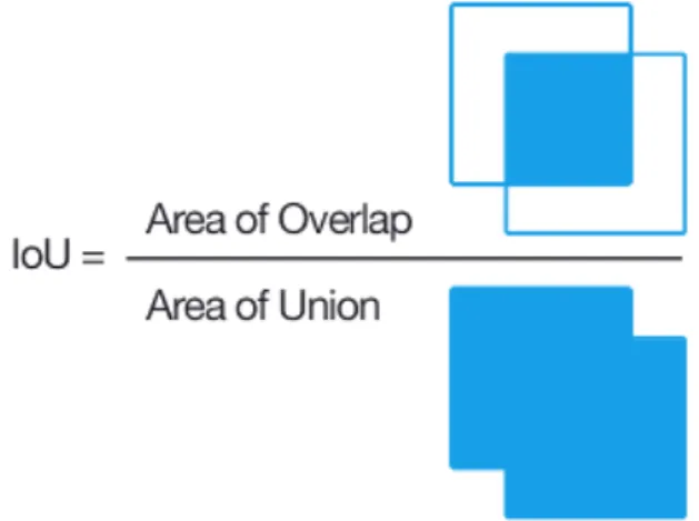
Intersection over union is an evaluation metric that returns the accuracy of a network that aims to detect objects into a given dataset. This kind of metric is usually used

(26)

for image detection with Convolutional Neural Networks, Recurrent Convolutional Neural Networks, YOLO[20], etc. It consists in the creation of a ground truth bounding box from the test images, and compare it with a bounding box created from the predictions, the ratio between the area of the overlap, by the union area between both of them, is the value that IoU displays. Figure 2.10 shows the equation in a 2D scenario for the use of IoU metric.

Figure 2.10: Definition of Intersection Over the union

As this metric is applied to 2D image recognition, it can also be used in 3D sce-narios, by adding a third axis and transforming the bounding box into a bounding cube, the basic idea remains the same. For the case of 3D point clouds, this results comes in handy, because it will represent if a predicted object is inside their correct space.

(27)

(28)

State of the Art

As mentioned before, PointNet is the backbone if this investigation, its main de-scription and architecture is the topic of this chapter, and also a review the current state of the art in point cloud segmentation is done, prior to start with the full development scenarios.

3.1 Segmentation-Instantiation for Point Clouds

State of the Art

As the time this investigation work is published, there is no current work on 3D point cloud instantiation, several architectures and research works about construction[21], urban deployment[22], pure point cloud segmentation[23] like PointNet, achieves good results for segmentation.

Instantiation in 2D however have several advances, being the one used for references in this work Deep Watershed Transform for Instance Segmentation[3], that achieves object image segmentation by using classical watershed transforms and modern deep learning to produce an energy map of the image where object instances are unam-biguously represented as energy basins.

3.1.1 Image Segmentation Instantiation

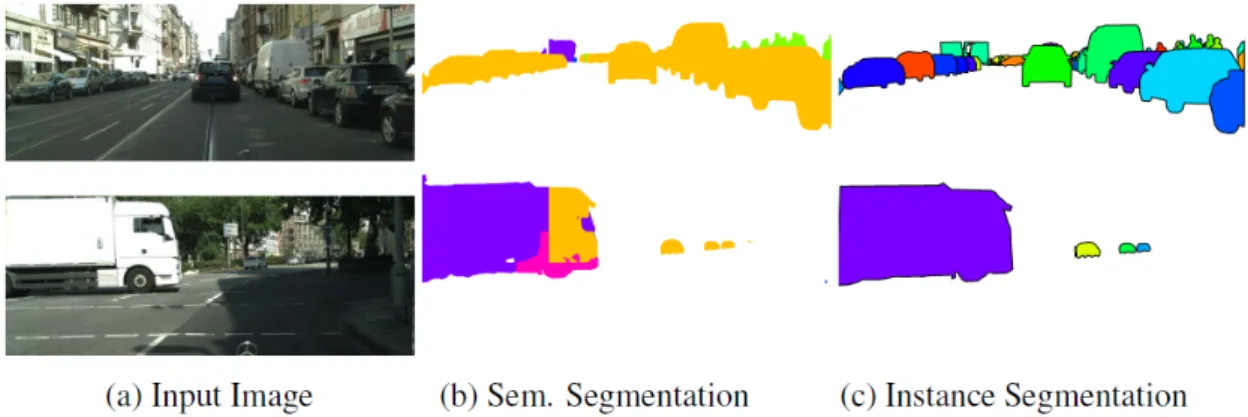
Image instantiation is now quite a solid topic, browsing for examples lead to numer-ous and very solid example, the basic idea is use deep learning techniques in contrast to initial approaches that used TextonForest and Random Forest based classifiers to achieve image segmentation, and feed this to a instantiation wise subnetwork as a second step. With deep learning, better results are achieved[24], the basic idea is

(29)

that each pixel is assigned to a class and an instance identity, thought convolutional neural networks and the use of boxes or watershed energy maps for example. After the complete learning process, the network identifies each element and its instance. Figure 3.1 contains a proposed architecture for a pixelwise semantic instantiation deep neural network.

Figure 3.1: Pixelwise example architecture from Pixelwise Instance Segmentation with a Dynamically Instantiated Network[24]

Aerial image interpretation is also a field that image segmentation has covered[25], with the recent blooming of drones, the personal retrieval for images and their ne-cessity to process them, had become imperative.

3.1.2 3D Segmentation Techniques

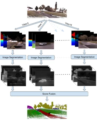
Segmentation also had been a wide topic inside the 3D world, it is represented as a difficult challenge, even for the new techniques on convolutional neural networks that had achieved great results in a broad aspect of investigation topics, and punctually on 2D image segmentation[26]. The main problem lies in the data itself, because a 3D point cloud does not have an neighborhood structure as it is on an image, and this leads to a process called voxelization on which the data suffers from a loss of spatial resolution and large memory requirements. SEGCloud: Semantic Segmen-tation of 3D Point Clouds[27] is the most relevant example of this architecture. There exist, several approaches that deal with this problems however, for exam-ple projecting the set of points into synthetic images, render attributes extracted from the point cloud and process these images by a CNN for image-based semantic segmentation[28], this approach reaches over 88% accuracy on the reported experi-ments, so it could be consider as an efficient method. Its representation is on figure 3.2.

(30)

Figure 3.2: The input point cloud is projected into multiple virtual camera views, generating virtual images, these images are preocessed by an CNN for semantic segmentation and the output prediction scores from all views are fused into a single prediction for each point.

As the data from 3D point clouds is sparse by definition, so another approaches uses sparse convolutional operations that process these sparse data more efficiently, and thus produce sparse convolutional networks called submanifold sparse convolu-tional networks (SSCNs).

Finally, the newest architecture for semantic segmentation for 3D point clouds is PointNet[4], which takes unordered point clouds as input, and learns to generalize relevant features of them.

3.2 PointNet

PointNet is a efficient and simple deep learning network that provides a unified architecture for applications related to 3D point clouds, its applications goes from object classification, part segmentation, to scene semantic parsing. Although, it does not contain instance segmentation, but according to its publication article results [4] it achieves strong performance on par or even better than state of the art for the

(31)

described applications before.

3.2.1 Description

It works by consuming unordered, invariant point clouds as input, this clouds are represented as a set of 3D points where each point is a vector that contains basic (x, y, z) coordinates, and also extra information, such as color (R, G, B) represen-tation in this case, normal values, distances between points, etc. and outputs class labels for the entire input or per point segment/part labels for each point of the input. The applications of PointNet are described in figure 3.3.

Figure 3.3: Use of PointNet. It is a unified architecture that learns both global and local point features, providing a simple, efficient and effective approach for a number of 3D recognition tasks

3.2.2 Architecture

The basic architecture of PointNet network is simple and a unified one, in the initial stages each point is processed identically and independently. In the basic setting each point is represented by just its three coordinates X, Y, Z. Additional dimen-sions may be added by computing normals and other local or global features.

It’s description is referenced in figure 3.4, the key module is the max pooling layer that acts as a symmetric function to aggregate information from all the points, a local and global information combination structure, and two joint alignment networks that align both input points and point features, with this information, the network learns a set of optimization criteria that selects relevant points and encodes the reason for their selection. In this investigation, we are interested on the segmentation part of PointNet and its further adding of instantiation.

(32)

Figure 3.4: PointNet Architecture

The resulting final fully connected layers of the network aggregate these learned optimal points into the global descriptor for the entire shape for shape classification, or are used to predict per point labels in shape segmentation.

(33)

(34)

Development

This section contains the description of the techniques, data pre processing and hardware used for the different experiments conducted along this investigation.

4.0.1 Software

The base framework/architecture for 3D point clouds deep learning used is Point-Net, which relies heavily on TensorFlow, an open source library design to handle large and complex mathematical operations, typically used in deep learning. These calculations are represented as nodes, and the edges between them, represent the multidimensional arrays used in each calculation, thus, TensorFlow represents all the operations by numerical data flow charts as represented in figure 4.1.

Figure 4.1: Dataflow computational graph[29]

TensorFlow was designed by Google, and was initially used just as internal re-source, but from 2015 it has Apache 2.0 Open Source license, making it Open Source

(35)

and continued like this up until the conclusion of this work, increasing its popularity by day, and growing with a vast supporting community, with over 26183 commits on GitHub and 1203 contributors.

Python is the programming language that works together with TensorFlow, it is having a lot of support inside the data science and deep learning community, mak-ing them the default choice tools used in this investigation.

For processing, preparation and cleaning of the data, several other libraries were ap-plied, Python libraries: NumPy1 for numeric and array manipulation, h5py2 python package that allows to store huge amounts of numerical data as HDF5 format data, and easily manipulate that data from NumPy.

Deep learning frameworks use computationally cost calculations, its complexity lies into the large calculation matrix data that they have to handle. TensorFlow allows to use the parallel computational power of the GPU, so all of the experiments in this investigation exploit this characteristic, they had been executed in the servers pro-vided by the Image Processing Group of the Universitat Politecnica de Catalunya, using CUDA and cuDNN3_{accelerated library of primitives for deep neural networks,}

which provide access to the GPU. For plotting and quantification of results R4 is used along with its ggplot library. Tensorboard 5 _{is used as support for native}

vi-sualization of the logs about training, validation, evaluation and testing processes executed on TensorFlow.

4.0.2 Hardware

The training of the models were executed remotely onto the cloud of servers provided by the Image Processing Group of the Universitat Politecnica de Catalunya, as there exists several options for it, the command issued always requested node 6, with the specifications detailed in table 4.1.

1_{http://www.numpy.org/} 2_{http://www.h5py.org/}

3_{https://developer.nvidia.com/cudnn} 4_{https://cran.r-project.org/}

(36)

Resource Detail

Node c6

CPU

Model (Arch) Intel Xeon 2.2GHz (x86 64)

Cores 20

RAM 156GB

GPU

Model GTX Titan Black Arch/Capability Kepler/3.5

GPUs 2

Cores 2880

RAM 6GB

Tables 4.1: Hardware details

These resources were remotely accessed via ssh protocol, always requesting a CPU with 4 cores, 16GB of RAM and one dedicated GPU with 6GB of VRAM.

4.0.3 Point Cloud dataset used

As in PointNet, Stanford 2D-3D-Semantics Dataset [30] where used as default un-ordered point cloud source, this dataset is a collection of 6 large-scale indoor areas that originate from 3 different buildings of mainly educational and office use. The data is represented as a collection of XYZ coordinates with their respective RGB colours, figure 4.2 represents a visualization of area 2.

(37)

4.1 Experiments

Four main experiments were conducted in this investigation, each of them has the objective to find the similarity between points that could lead to identify them as a single object, and thus, achieving instantiation.

4.1.1 Preprocessing

The raw data from Stanford Dataset comes in a form of plain text archives, each one containingXY ZRGB information, and organized in hierarchical way from Area to room type6 to object7.

The main interest is to learn how to instantiate objects, so an initial exploration of the quantity of the objects contained in the dataset is needed, these results are shown in table 4.2.

Object Count Percentage board 3882 40% wall 1548 16% floor 1363 14% sofa 583 6% table 543 6% chair 455 5% ceiling 385 3% door 284 3% bookcase 254 3% clutter 168 2% beam 159 2% window 137 1% column 55 1%

Tables 4.2: Total count of objects in Stanford Dataset

As the results shown, the less recurrent object is column. For the experiments just those objects that are present more than 2% into the total count of the dataset are taken into account, the ones below these threshold are considered non represen-tative. Also objects like boards, ceilings and floors are considered too much alike and could mislead the network predictions, just walls had been preserved as they are the second most present objects, the objective of this is simplify the experiments,

6_{Room types are: conference room, office, auditorium, copy room, lounge, lobby, wc, hallway,}

pantry, storage and open space.

7_{Objects are: ceiling, floor, wall, beam, column, window, door, table, chair, sofa, bookcase,}

(38)

without losing too much information.

4.1.2 Data Sub setting

For the experiment scenarios, the total point cloud data is divided then into Areas 1-4 for training, Area 5 for validation and Area 6 for testing, the idea is to evaluate the model against a never before seen data. First a check on the class distribution of each one of them is done, to detect any unbalancing. The results are shown on figure 4.3.

Figure 4.3: Areas object balance count

The data tends to follow the same distribution, but it is notorious that in Area 5 the object table has a different value with respect to the others, in this case as it is just one value, I keep working with it anyway. Once the data is checked and divided, the experiments could be conducted.

(39)

4.1.3 Data generation

The initial assumption taken, is that the network could learn and generalize relevant parameters of the data, in this case, a relevant parameter needed for the first part of the investigation, is the relationship that the points have between them in the space, in other words their distance, to be able to separate them as independent objects. In order to prepare the data for the network, a label D is added to each one of the rows, this valueD is the euclidean distance taken from the center of the point cloud object to each point, normalized in 13 classes, with values from 0 to 12. The normalized scale were taken based on the initial PointNet segmentation predicted labelL, which has 13 value. Being PointNet the backbone of the network, this classification result logical.

Finally, the value D is going to be used as input in different ways along the ex-periments. A visualization sample of how the points are distributed in one scene is shown in figure 4.4,

Figure 4.4: Distribution of points from the centroid of the object

Once again, if we quantify the distribution of the points into the selected dataset as in figure 4.5, we observe that there is an unbalance for the center and external points, in this case this results make sense, because the distance metric used.

(40)

Figure 4.5: Histogram with the distribution of the 13 D classes in the dataset To deal with large amounts of data, all the filtered input is then formatted into h5 format, using pythons’ h5py library, this is the final input data used to train, validate and test the network. To boost the learning process, three more columns are added to this files, containing the normalized values of theXY Z coordinates.

Once the prediction is done, a point cloud dump of the ground truth and the prediction is available to better identify the predicted distances, each one of them had been coloured according to its rank, as shown in figure 4.6.

Figure 4.6: Coloured point cloud with its RGB values. Each distance had been normalized in the range [0,12], being the center 0 and the borders 12

(41)

4.1.4 Architecture Modifications

The objective of predict the distance D, is to try to establish the bounding points of the object, and the use them to differentiate one object from another, the main modifications done in PointNet architecture, lies in the tensor size and pre process-ing, the original architecture accepts tensors of size nx3, being n the number of points on each

4.1.5 Experiments Scenarios

Four main scenarios are created, starting from the initial assumption that PoinNet is indeed learning a set of optimization criteria that selects the most relevant points of the cloud. These scenarios were progressively and sequentially developed as the investigation continue, these scenarios are are: reason for their selection

• Replacement of the predicted L parameter into the original network by the euclidean distance obtained D and predict D.

• Replace the value of R in the RGB input values of the dataset by L and predict D

• Add L as input network value, to predictD.

• ReplaceRGB original values with the colour code of the normalized distances and add L as input network value, to predictD.

4.1.6 Training Process

With the proper division of the train, validation and evaluation dataset, all the scenarios were executed with the configuration presented in 4.3

Object Configuration

Loss Function Softmax Cross Entropy Epoch 250

Dropout value 0.7

Weight Initialization Xavier Initialization

Tables 4.3: Hyperparameter values and configurations run for all experiments, sev-eral other cases were tested, the values presented in this table are the most accurate ones, based on accuracy and loss onto the test, validation and test executions.

(42)

Results

This chapter contains the detail results for the scenarios previously explained for this investigation. For each one of them, the results are presented using different visual and numerical resources, a plot for the results obtained in validation, train, test and evaluation of each epoch is first presented to better recognize the tendency, classification results table contain the detail about each one of the classes classifi-cation data in the model, and finally a coloured visualization of the ground truth and predicted points, to be more human friendly about the point prediction in the scenarios. More details about the first and last results for each epoch output aids to see if the initial scenario had been improved through the full cycle, as well as logs of the process training into TensorFlow, visualized with TensorBoard, could be found in the Appendix section.

5.1 First Scenario

The first scenario presents the basic implementation of the network, to test the hypothesis presented by PointNet. In this case, a Tensor of sizeB x Point Number x 9, using Xavier weight initialization.

(43)

5.1.1 Accuracy vs Epoch plot

Figure 5.1: Results for Scenario 1, contains a) the train results, b) validation set, c) evaluation of each epoch, d) train results. For a), b), and c) the x coordinates represent the number of epochs, d) contains the number of models used in test.

(44)

Class GT Classes Positive

Classes

True Positive

Classes Precision Recall

IOU Accuracy 0 13755 1819 1171 0.64 0.08 0.0813 1 51721 51946 25402 0.49 0.49 0.3246 2 99636 89762 44634 0.49 0.45 0.3083 3 144904 137100 67416 0.49 0.46 0.3142 4 184878 190037 92925 0.49 0.50 0.3295 5 209893 208095 102320 0.49 0.48 0.3241 6 211814 221840 104506 0.47 0.49 0.3175 7 198844 195896 93551 0.48 0.47 0.3106 8 178237 187537 86280 0.46 0.48 0.3087 9 157771 159968 76428 0.47 0.49 0.3167 10 128586 141563 66488 0.47 0.51 0.3265 11 92327 68718 37943 0.55 0.41 0.3082 12 60242 78327 40592 0.52 0.68 0.4143 Overall Accuracy 0.4846

Tables 5.1: Evaluation of classification for scenario 1

5.1.3 Ground truth and prediction plot

Predicted values were not as good as expected, in future modifications of the data or/and the architecture, one of the prior tasks will be improving this accuracy. This first scenario, is most time consuming one of them all, represent the basis on which parameters had been tuned to obtained the fittest result.

(a) (b)

(45)

5.2 Second Scenario

The initial conditions are basically the same that in scenario 1, but as the result were not as expected there, a modification into the values of the input has made, changing the value of R in the RGB values to the label value of the object.

5.2.1 Accuracy vs Epoch plot

(46)

5.2.2 Accuracy per class

Classes

True Positive

5.2.3 Ground truth and prediction plot

Scenario 2 does not shown an improvement in results, the first idea for scenario 1 remains. But it is clear that PointNet it is somewhat successful in generalizing relevant point.

(a) (b)

(47)

5.3 Third Scenario

For the third and fourth scenarios, the data generator and the network where mod-ified, now the input for the network is a Tensor of size B x Point Number x 10, including the value L representing the label class of the object, and outputting a predicted value ofD that is the distance.

5.3.1 Accuracy vs Epoch plot

(48)

5.3.2 Accuracy per class

Classes

True Positive

5.3.3 Ground truth and prediction plot

Third scenario presents the less accurate results, this is surprising to the initial assumptions made, in this case, the original architecture were modified, and more data are added, but the results were poorer, to test if this modification are wrong, a fourth scenario is created and tested.

5.4 Fourth Scenario

The fourth scenario takes as input, the RGB values stated in the colour code ex-plained before, this case was a concept to test if the modified version of the network is correct, because in initial assumptions taken, adding the values of the segmenta-tion labelL to the input of the network, will result in a better generalization of the model, but the results proven contrary.

(49)

(a) (b)

(50)

5.4.1 Accuracy vs Epoch plot

(51)

Classes

True Positive

Results here proven that the previous scenario modifications were correct, the data has been augmented making the network to overfit.

5.4.3 Ground truth and prediction plot

After conducting all the experiments, it is useful to present a condensed result comparison between them, the values for the overall accuracy obtained on each test set are in table 5.5.

Scenario 1 Scenario 2 Scenario 3 Scenario 4 Overall Accuracy Overall Accuracy Overall Accuracy Overall Accuracy

0.5 0.42 0.38 1.0

(52)

(a) (b)

Figure 5.8: Ground truth (a) and Prediction (b) values for scenario 4

As summarized in each scenario, highest accuracy was achieved in scenario 1, from all the evaluation tables from all of them but 4, the accuracy of the values of the center points of each object is among the lowest, one possible explanation for this is that the area of these points is far small that the surrounding ones, so the network can not generalize well.

(53)

(54)

Discussions, Conclusions and

Future Work

6.1 Discussions

The conducted experiments scenarios identified scenario 4 as the one with the high-est accuracy, but this results are misleading, because the neural network is feed with data that has previously been altered, this is just done for testing if the modifica-tions of the network were correct, in early stages of the investigation, an assumption was made: augmenting the data, by giving the segmentation labelLas an input to the network will achieve better results; on this premise, scenario 3 was created, but due to the low values obtained from the experiment, this conclusion was proven to be wrong, and needed to be formally denied.

While the results of 3 out of 4 experiments were not present satisfactory results, scenario number 1 could be considered as partially successful, and could be the can-didate to prior experimentation, or could be improved by applying a different metric technique for the point distance.

Saturation of the epoch training proven to be useful, but the threshold on which the values maintain during all the training process was always steady after a while, in this cases the adding or subtracting of data proven to alter the results in small quantities, so with more data for training, the results will improve onto the same model.

6.2 Conclusions

The multiple scenarios proposed for this project had the objective of identify a method that could lead to identify objects and its classes, parting from the cases

(55)

that a group of points in the cloud could be part of an object having the same semantic class or could not be part of the same object but could have the same se-mantic class, then this information will lead to the application of a similarity metric between the instance labels obtained and the semantic labels obtained from Point-Net, and thus achieving instantiation.

Results obtained from each model, showed that relevant features could be extracted from the approach of measuring the euclidean distance between points, this features reaches 50% accuracy at most, but the values are a good start to apply an instan-tiation process.

Hyper parameters proven to be determinant in the training process, in early stages of the experiments, the size of the mini batches feed to the network were bigger, and the results achieved 37% accuracy at most, in latest stages this value were reduced. Data pre processing and checking is fundamental, varying the test, train and val-idation sets after the data was clear of imbalances had minimum impact onto the model.

With the obtained results in scenario 1, point cloud instantiation has promising results, and PointNet proven to learn relevant features of the data.

6.3 Future Work

Instantiation had not been achieved in this investigation work, the values have promising future results, and the obvious next step in this investigation is to im-prove the generalization value of the network, and add a similarity metric on the obtained data to instantiate the objects. Different metrics applied to the calculation of distances between the points in the point cloud could improve the results as well, perhaps with the application of a distance matrix for all the points and a subsequent feeding of this matrix to the network , will help for it to learn to generalize several parameters.

(56)

[1] Google Corporation. Google quickdraw.

[2] Phillip Isola, Jun-Yan Zhu, Tinghui Zhou, and Alexei A Efros. Image-to-image translation with conditional adversarial networks. arXiv preprint arXiv:1611.07004, 2016.

[3] Min Bai and Raquel Urtasun. Deep watershed transform for instance segmen-tation. In2017 IEEE Conference on Computer Vision and Pattern Recognition (CVPR), pages 2858–2866. IEEE, 2017.

[4] Charles R Qi, Hao Su, Kaichun Mo, and Leonidas J Guibas. Pointnet: Deep learning on point sets for 3d classification and segmentation. arXiv preprint arXiv:1612.00593, 2016.

[5] Lars Linsen. Point cloud representation. Univ., Fak. f¨ur Informatik, Bibliothek, 2001.

[6] PointCab GmbH 2017. Point clouds from drones (uav – unmanned aerial vehi-cle), 2014.

[7] A KEITH Turner, JOHN Kemeny, SEIFKO Slob, and ROBERT Hack. Evalu-ation, and management of unstable rock slopes by 3-d laser scanning. Interna-tional association for engineering geology and the environment. The Geological Society of London, pages 1–11, 2006.

[8] Yann LeCun, Yoshua Bengio, and Geoffrey Hinton. Deep learning. Nature, 521(7553):436–444, 2015.

[9] Ian Goodfellow, Yoshua Bengio, and Aaron Courville. Deep Learning. MIT Press, 2016. http://www.deeplearningbook.org.

[10] Jeff Donahue, Yangqing Jia, Oriol Vinyals, Judy Hoffman, Ning Zhang, Eric Tzeng, and Trevor Darrell. Decaf: A deep convolutional activation feature for generic visual recognition. In International conference on machine learning, pages 647–655, 2014.

(57)

[11] Angel Alfonso Cruz-Roa, John Edison Arevalo Ovalle, Anant Madabhushi, and Fabio Augusto Gonz´alez Osorio. A deep learning architecture for image rep-resentation, visual interpretability and automated basal-cell carcinoma can-cer detection. In International Conference on Medical Image Computing and Computer-Assisted Intervention, pages 403–410. Springer, 2013.

[12] Xiao Ding, Yue Zhang, Ting Liu, and Junwen Duan. Deep learning for event-driven stock prediction. InIjcai, pages 2327–2333, 2015.

[13] Frank Rosenblatt. Principles of neurodynamics. 1962.

[14] Bernard Widrow and Marcian E Hoff. Adaptive switching circuits. Technical report, STANFORD UNIV CA STANFORD ELECTRONICS LABS, 1960. [15] Bernard Widrow, Samuel D Stearns, and John C Burgess. Adaptive signal

processing edited by bernard widrow and samuel d. stearns. The Journal of the Acoustical Society of America, 80(3):991–992, 1986.

[16] Paul John Werbos. Beyond regression: New tools for prediction and analysis in the behavioral sciences. Doctoral Dissertation, Applied Mathematics, Harvard University, MA, 1974.

[17] Siddharth Krishna Kumar. On weight initialization in deep neural networks.

arXiv preprint arXiv:1704.08863, 2017.

[18] D Randall Wilson and Tony R Martinez. The general inefficiency of batch train-ing for gradient descent learntrain-ing. Neural Networks, 16(10):1429–1451, 2003.

[19] Tijmen Tieleman and Geoffrey Hinton. Lecture 6.5-rmsprop: Divide the gradi-ent by a running average of its recgradi-ent magnitude.COURSERA: Neural networks for machine learning, 4(2):26–31, 2012.

[20] Joseph Redmon, Santosh Divvala, Ross Girshick, and Ali Farhadi. You only look once: Unified, real-time object detection. In Proceedings of the IEEE Conference on Computer Vision and Pattern Recognition, pages 779–788, 2016. [21] Joachim Bauer, Konrad Karner, Andreas Klaus, Christopher Zach, and Konrad Schindler. Segmentation of building models from dense 3D point-clouds. na, 2003.

[22] Jorge Hern´andez and Beatriz Marcotegui. Point cloud segmentation towards urban ground modeling. In Urban Remote Sensing Event, 2009 Joint, pages 1–5. IEEE, 2009.

[23] Patrik Tosteberg. Semantic segmentation of point clouds using deep learning, 2017.

[24] Anurag Arnab and Philip HS Torr. Pixelwise instance segmentation with a dynamically instantiated network. arXiv preprint arXiv:1704.02386, 2017.

(58)

[25] Wolfgang F¨orstner and Lutz Pl¨umer. Semantic Modeling for the Acquisition of Topographic Information from Images and Maps: SMATI 97. Springer Science & Business Media, 1997.

[26] Jonathan Long, Evan Shelhamer, and Trevor Darrell. Fully convolutional net-works for semantic segmentation. In Proceedings of the IEEE Conference on Computer Vision and Pattern Recognition, pages 3431–3440, 2015.

[27] Lyne P Tchapmi, Christopher B Choy, Iro Armeni, JunYoung Gwak, and Silvio Savarese. Segcloud: Semantic segmentation of 3d point clouds. arXiv preprint arXiv:1710.07563, 2017.

[28] Felix J¨aremo Lawin, Martin Danelljan, Patrik Tosteberg, Goutam Bhat, Fa-had Shahbaz Khan, and Michael Felsberg. Deep projective 3d semantic seg-mentation. arXiv preprint arXiv:1705.03428, 2017.

[29] T. Hope, Y.S. Resheff, and I. Lieder.Learning TensorFlow: A Guide to Building Deep Learning Systems. O’Reilly Media, 2017.

[30] I. Armeni, A. Sax, A. R. Zamir, and S. Savarese. Joint 2D-3D-Semantic Data for Indoor Scene Understanding. ArXiv e-prints, February 2017.

(59)

(60)

(61)

(62)

Tensorboard scalars log output

Figure 1: Tensorboard output when the value to predict is the euclidean distanceD

(63)

class precision recall f1-score support 0.0 0.64 0.08 0.15 14227 1.0 0.49 0.49 0.49 53221 2.0 0.49 0.45 0.47 102909 3.0 0.49 0.46 0.48 149791 4.0 0.49 0.50 0.49 190534 5.0 0.49 0.48 0.49 216206 6.0 0.47 0.49 0.48 219978 7.0 0.48 0.47 0.47 207074 8.0 0.46 0.48 0.47 186278 9.0 0.47 0.49 0.48 164740 10.0 0.47 0.51 0.49 133972 11.0 0.55 0.41 0.47 95749 12.0 0.52 0.68 0.59 63465 avg / total 0.48 0.48 0.48 1798144 Tables 1: Evaluation of classification for scenario 1

(64)

Figure 2: Tensorboard output when the value ofR had been replaced with L

(65)

(66)

Figure 3: Tensorboard output when the value of Lhad been added to the network input

(67)

(68)

Figure 4: Tensorboard output when the value of L and custom RGB had been added to the network input

(69)

Instance Segmentation of Point Clouds using Deep Learning