OPTIMIZATION OF EDM PARAMETERS USING TAGUCHI METHOD AND GREY RELATIONAL ANALYSIS FOR MILD STEEL IS 2026

(1)

Copyright to IJIRSET www.ijirset.com

3095

OPTIMIZATION OF EDM PARAMETERS

USING TAGUCHI METHOD AND GREY

RELATIONAL ANALYSIS FOR MILD

STEEL IS 2026

Raghuraman S1, Thiruppathi K2, Panneerselvam T3, Santosh S4

Professor, School of Mechanical Engineering, SASTRA University, Thanjavur, Tamil nadu, India1

Senior Assistant Professor, School of Mechanical Engineering, SASTRA University, Thanjavur, Tamil nadu, India2,3

UG Student, School of Mechanical Engineering, SASTRA University, Thanjavur, Tamil nadu, India4

Abstract: Optimization is one of the techniques used in manufacturing sectors to arrive for the best manufacturing conditions, which is an essential need for industries towards manufacturing of quality products at lower cost. This paper aims to investigate the optimal set of process parameters such as current, pulse ON and OFF time in Electrical Discharge Machining (EDM) process to identify the variations in three performance characteristics such as rate of material removal, wear rate on tool, and surface roughness value on the work material for machining Mild Steel IS 2026 using copper electrode. Based on the experiments conducted on L9 orthogonal array, analysis has been carried out using Grey Relational Analysis, a Taguchi method. Response tables and graphs were used to find the optimal levels of parameters in EDM process. The confirmation experiments were carried out to validate the optimal results. Thus, the machining parameters for EDM were optimized for achieving the combined objectives of higher rate of material removal, lower wear rate on tool, and lower surface roughness value on the work material considered in this work. The obtained results show that the Taguchi Grey relational Analysis is being effective technique to optimize the machining parameters for EDM process.

Keywords: Electrical Discharge Machining, Orthogonal Array, Signal-to-Noise ratio, Grey Relational Analysis

I. INTRODUCTION

The quality of a product is the main factor for showing growth of a company. The quality of the product mainly depends upon the material and process parameters. Optimization technique plays a vital role to increase the quality of the product [1]. Hence, many authors have presented their works on the optimisation of process parameters for various machining processes. S. Dhanabalan and K Sivakumar have done EDM process optimization with multiple performance characteristics based on orthogonal array with grey relational analysis for Titanium grades with brass electrode[2]. Saha and Choudhury studied the process of dry EDM with tubular copper tool electrode and mild steel work-piece [3].

Grey relational analysis (GRA) has been used by many researchers for machining processes which include electric discharge machining [4], chemical mechanical polishing [5], determining condition of tool in turning [6], side milling [7], and flank milling [8] to analyse the performance of diamond tool carbide inserts in dry turning [9], and optimization of parameters in drilling [10].

The objective of this paper is to determine the optimal levels of the process parameters for Electric-Discharge Machining process using Taguchi approaches. This work was done with Mild Steel IS 2026 grade as work piece material and copper as tool electrode. Signal-to-Noise ratio analysis and Grey relational analysis were applied to obtain the optimum values of the process parameters for the formation of a blind hole of 10 mm diameter and 3 mm depth. The process parameters such as peak current, pulse on time and pulse off time were optimized with the considerations of multiple performance characteristics such as material removal rate, tool wear rate and surface roughness value on the work material.

II. MATERIALS AND METHODS USED

A. Material and machine

(2)

3096

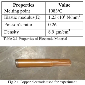
Properties Value

Melting point 1083ºC

Elastic modulus(E) 1.23×105 N/mm2 Poisson‟s ratio 0.26

Density 8.9 gm/cm3

Table 2.1 Properties of Electrode Material

Fig 2.1 Copper electrode used for experiment

Machining was carried out in EDM machine of ELECTRONICA Machine tools Ltd at Shanmugha Precision Forgings (SPF), Thanjavur as shown in Fig 2.2. Machine is provided with fixed pulse voltage. The current, pulse ON time and pulse OFF time were selected from the range. Table 2.2 shows the Machine specifications and Table 2.3 shows the working conditions and description of EDM.

Description Details

Supply voltage 75V

Discharge current 30A

Servo system Electromechanical

Power consumption 2kW

Model ELECTRONICA

Table 2.2 Machine specifications

Fig 2.2EDM machine

Table 2.3 Working conditions and description of EDM

Working conditions Description

Work piece Mild steel IS2026

Electrode Copper

(3)

3097 The control parameters at three different levels and three different response parameters considered for multiple performance characteristics in this work [11] are shown in Table 2.4.

Response Parameters

Material Removal Rate (mm3 /min.) Tool Wear Rate (mm3 /min.) Surface Roughness (µm)

Control Parameters

Levels

1 2 3

Discharge current (A) 10 18 26

Pulse ON time (µs) 11 55 95

Pulse OFF time (µs) 5 7 9

Table 2.4 Response parameters and control parameters with their levels

B. Experimental details

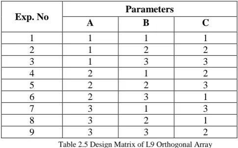
Design of experiment is an effective tool to design and conduct the experiments with minimum resources. Orthogonal Array is a statistical method of defining parameters that converts test areas into factors and levels. Test design using orthogonal array creates an efficient and concise test suite with fewer test cases without compromising test coverage. In this work, L9 Orthogonal Array design matrix is used to set the control parameters to evaluate the process performance. The Table 2.5 shows the design matrix used in this work.

Table 2.5 Design Matrix of L9 Orthogonal Array

A hole of 10mm diameter and 3 mm depth was produced by EDM process with the help of copper electrode on mild steel IS 2026 as work piece material for each combination of parameters considered according to the Orthogonal Array. The work piece and tool electrode were weighed before and after the machining by using the electronic weigh-balance to calculate the material removal rate and the tool wear rate. The surface roughness of the holes machined was evaluated using a surface roughness-testing machine.

B.1. Material removal rate

The material removal rate of the work piece is the volume of the material removed per minute. It can be calculated using the following relation.

(

) 1000

(

)

i f

w

W

MRR

D

t









(1)

MRR

– Material Removal Rate (mm3/min)

Wi

- Initial weight of work piece (gm)

Wf

- Final weight of work piece (gm)

D

w - Density of the work piece (gm/cm3)

t

- Period of trial (min)

B.2Tool wear rate

Exp. No Parameters

A B C

1 1 1 1

2 1 2 2

3 1 3 3

4 2 1 2

5 2 2 3

6 2 3 1

7 3 1 3

8 3 2 1

(4)

3098 The tool wear rate (TWR) of the electrode is the amount of the tool wear per minute. It can be calculated using the following equation.

(

) 1000

(

)

i f

e

T

TWR

D

t









(2)

TWR - Tool wear rate (mm3/min) Ti - Initial weight of tool (gm) Tf - Final weight of tool (gm) De - Density of the tool (gm/cm3) t - Period of trial (min)

B.3 Surface roughness

Roughness is often a good predictor of the performance of a mechanical component, since irregularities in the surface may form nucleation sites for cracks or corrosion [12]. Roughness is a measure of the texture of a surface. It is quantified by the vertical deviations of a real surface from its ideal form. If these deviations are large, the surface is rough; if small, the surface is smooth. Roughness is typically considered to be the high frequency, short wavelength component of a measured surface.

The parameter mostly used for general surface roughness is Ra. It measures average roughness by comparing all the peaks and valleys to the mean line, and then averaging them all over the entire cut-off length. The surface roughness can be measured using a surface roughness tester machine, which is shown in Fig.2.3.

Fig 2.3 Equipment for Surface Roughness Measurement

III. ANALYSIS OF EXPERIMENTS

The experiments were conducted based on varying the process parameters, which affect the machining process to obtain the required quality characteristics. Quality characteristics are the response values or output values expected out of the experiments. There are 64 such quality characteristics. The most commonly used are:

1) Larger the better 2) Smaller the better 3) Nominal the best 4) Classified attribute 5) Signed target

As the objective is to obtain the high material removal rate (MRR), low tool wear rate, and best surface finish, it is concerned with obtaining larger value for MRR, smaller value of tool wear rate and smaller value of surface roughness. Hence, the required quality characteristic for high MRR is larger the better, which states that the output must be as large as possible, and for tool wear rate and surface roughness is smaller the better, which states that the output must be as low as possible.

A. Experimental Results

(5)

3099 Exp. No Current (A) Pulse ON Time (µs) Pulse OFF Time (µs) MRR (mm3/min)

TWR (mm3/min)

Surface Roughness (µm)

1 10 11 5 3.754 0.130 4.329

2 10 55 7 10.451 0.178 12.541

3 10 95 9 15.006 0.244 6.494

4 18 11 7 21.256 0.147 3.932

5 18 55 9 32.412 0.274 10.982

6 18 95 5 35.430 0.323 8.484

7 26 11 9 25.452 0.240 4.588

8 26 55 5 43.517 0.372 14.219

9 26 95 7 48.775 0.448 10.242

Table 3.1 Experimental results

B. Optimization using Grey Relational Analysis

Taguchi's method [13] is focused on the effective application of engineering strategies rather than advanced statistical techniques. The primary goals of Taguchi method are

 A reduction in the variation of a product design to improve quality and lower the loss imparted to society.  A proper product or process implementation strategy, which can further reduce the level of variation. The steps involved in Taguchi‟s Grey Relational Analysis are:

STEP 1- : The transformation of S-N Ratio values from the original response values was the initial step. For that the equations of „larger the better‟, „smaller the better‟ and „nominal the best‟ were used. Subsequent analysis was carried out on the basis of these S/N ratio values. This is shown in table 3.2.

Type 1:

/

_HB

10 log [( )(

₁₀

1

₂

)]

ij

S N

n

Y

 



(3)

Type 2:

2

10

/

_LB

10 log [

Y

ij

]

S N

n

 



(4)

Type 3:

S N

/

_NB

10 log [

₁₀

1

₂

]

S



(5)

Where Yij is the value of the response

„j‟ in the ith_{experiment condition, with i=1, 2, 3,…n; j = 1,2…k} and S2 are the sample mean and variance

Exp No

Response values S/N ratios

MRR (mm3/min)

TWR (mm3/min)

SR (µm) MRR (dB) TWR (dB) SR (dB)

1 03.754 0.130 04.329 11.490 17.741 -12.728

2 10.451 0.178 12.541 20.383 14.992 -21.967

3 15.006 0.244 06.494 23.525 12.245 -16.250

4 21.256 0.147 03.932 26.550 16.654 -11.892

5 32.412 0.274 10.982 30.214 11.245 -20.814

6 35.430 0.323 08.484 30.987 09.816 -18.572

7 25.452 0.240 04.588 28.114 12.381 -13.232

8 43.517 0.372 14.219 32.773 08.601 -23.057

9 48.775 0.448 10.242 33.764 06.976 -20.208

Table 3.2Signal-to-Noise ratios

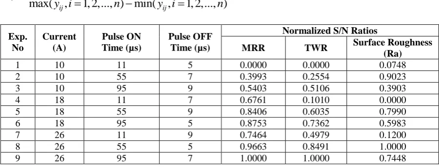
STEP 2 : - In the 2nd step of the grey relational analysis [14], pre-processing of the data was first performed for normalizing the raw data for analysis. This is shown in Table 3.3. Yij is normalized as Zij (0 ≤ Zij ≤ 1) by the following

formula to avoid the effect of adopting different unitsand to reduce the variability. The normalized output parameter corresponding to the larger-the-better criterion can be expressed as







y

i

n





y

i

n



n

i

y

Zij

ij ij ij ij

....

2 ,

1 ,

min

,....

2 ,

1 ,

max

,....

2 ,

1 ,

min









(6)

3100 Then for the output parameters, which follow the lower-the-better criterion can be expressed as

max(

,

1, 2,..., )

max(

,

1, 2,..., ) min(

,

1, 2,..., )

ij ij

y i

n

y

Zij

y i

n

y i

n











(7)

Exp. No Current (A) Pulse ON Time (µs) Pulse OFF Time (µs)

Normalized S/N Ratios

MRR TWR Surface Roughness

(Ra)

1 10 11 5 0.0000 0.0000 0.0748

2 10 55 7 0.3993 0.2554 0.9023

3 10 95 9 0.5403 0.5106 0.3903

4 18 11 7 0.6761 0.1010 0.0000

5 18 55 9 0.8406 0.6035 0.7990

6 18 95 5 0.8753 0.7362 0.5983

7 26 11 9 0.7464 0.4979 0.1200

8 26 55 5 0.9663 0.8491 1.0000

9 26 95 7 1.0000 1.0000 0.7448

Table 3.3 Normalized Signal-to-Noise ratios

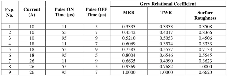
STEP 3: The grey relational coefficient [15] is calculated to express the relationship between the ideal (best) and actual normalized experimental results. Before that the deviation sequence for the reference and comparability sequence were found out. These are given in Table 3.4 and grey relational coefficient is given in Table 3.5. The grey relational coefficient can be expressed as

min max 0 max

( )

i i

k









 





 

(8)

Where,



₀i

( )

k

is the deviation sequence of the reference sequence and comparability sequence.

 

k

y

   

k

y

_i

k

i







₀ ₀ (9)

 

k

y

 

k

y

k

i

j







j







_{m in}

min

₀ (10)

 

k

y

 

k

y

k

i

j







j







m ax 0

max

(11)

y k

₀

( )

denotes the sequence and

y k

_j

( )

denotes the comparability sequence. ζ is distinguishing or identified coefficient. The value of ζ is the smaller and the distinguished ability is the larger. ζ = 0.5 is generally used.

Step 4: The grey relational grade was determined by averaging the grey relational coefficient corresponding to each performance characteristic [16]. It is given in the Table 3.6. The overall performance characteristic of the multiple response process depends on the calculated grey relational grade.The grey relational grade can be expressed as

1

1 ( )

n i i k

k

n









(12)

(7)

3101 Table 3.4 Deviation sequences

Table 3.5Grey Relational Co-efficient

Table 3.6Grey Relational Grade

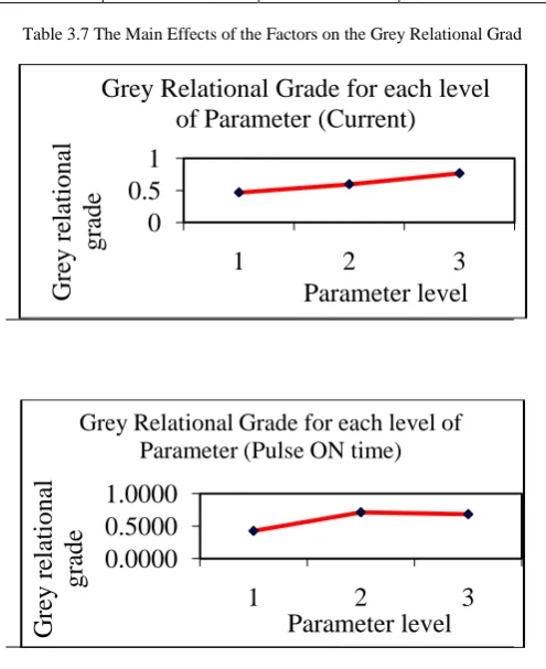
Step 5: Determination of the Optimal Factor and its Level Combination. The Fig. 3.1 shows theGrey relational grades [17] for maximum MRR, minimum TWR and minimum Ra. Since the experimental design is orthogonal, it is possible to separate out the effect of each machining parameter on the grey relational grade at different levels [18]. For example, the mean of the grey relational grade for the pulse current at levels 1, 2 and 3 can be calculated by averaging the grey relational grade for the experiments 1 to 3, 4 to 6, and 7 to 9 respectively. The mean of the grey relational grade for each level of the machining parameters is summarized and shown in Table 3.7

Exp. No.

Current (A)

Pulse ON

Time (µs)

Pulse OFF Time (µs)

Deviation Sequences

MRR TWR Surface

Roughness

1 10 11 5 1.0000 1.0000 0.9252

2 10 55 7 0.6007 0.7446 0.0977

3 10 95 9 0.4597 0.4894 0.6097

4 18 11 7 0.3239 0.8990 1.0000

5 18 55 9 0.1594 0.3965 0.2010

6 18 95 5 0.1247 0.2638 0.4017

7 26 11 9 0.2536 0.5021 0.8800

8 26 55 5 0.0337 0.1509 0.0000

9 26 95 7 0.0000 0.0000 0.2552

Exp. No.

Current (A)

Pulse ON Time (µs)

Pulse OFF Time (µs)

Grey Relational Coefficient

MRR TWR Surface

Roughness

1 10 11 5 0.3333 0.3333 0.3508

2 10 55 7 0.4542 0.4017 0.8366

3 10 95 9 0.5210 0.5053 0.4506

4 18 11 7 0.6069 0.3574 0.3333

5 18 55 9 0.7583 0.5577 0.7133

6 18 95 5 0.8004 0.6546 0.5545

7 26 11 9 0.6635 0.4990 0.3623

8 26 55 5 0.9369 0.7682 1.0000

9 26 95 7 1.0000 1.0000 0.6620

Exp. No Current (A) Pulse ON

Time (µs)

Pulse OFF Time(µs)

Grey Relational

Grade Rank

1 1 1 1 0.3392 9

2 1 2 2 0.5642 5

3 1 3 3 0.4923 7

4 2 1 2 0.4325 8

5 2 2 3 0.6764 3

6 2 3 1 0.6699 4

7 3 1 3 0.5082 6

8 3 2 1 0.9017 1

(8)

3102 Fig.3.1Grey Relational Grades for Maximum MRR, Minimum TWR and Minimum Ra

The larger the grey relational grade [19], the better is the multiple performance characteristics. However, the relative importance among the machining parameters for the multiple performance characteristics still needs to be known, so that the optimal combinations of the machining parameter levels can be determined more accurately. With the help of Fig.3.2and Table 3.7, the optimal parameter combination was determined as A3 (pulse current, 26A), B2 (pulse on time, 55μs) and C1 (pulse off time, 5μs).

Parameters Level 1 Level 2 Level 3 Max-Min Rank

Current 0.4652 0.5929 0.7637* 0.2985 1

Pulse on 0.4267 0.7120* 0.6832 0.2853 2

Pulse off 0.6348* 0.6280 0.5590 0.0758 3

Table 3.7 The Main Effects of the Factors on the Grey Relational Grad

0.000 0.100 0.200 0.300 0.400 0.500 0.600 0.700 0.800 0.900 1.000

1 2 3 4 5 6 7 8 9

Gre

y

re

latio

n

al g

ra

d

e

Experimental run Grey Relational Grade

0

0.5

1

2

3 Gr

ey

re

lational

gr

ade

Parameter level

Grey Relational Grade for each level

of Parameter (Current)

0.0000

0.5000

1.0000

1

2

3 G

re

y

r

ela

tiona

l

gr

ade

Parameter level

Grey Relational Grade for each level of

(9)

3103 Fig. 3.2 Grey relational grade for each level of parameters

C. Confirming Results

The confirmation test for the optimal parameters with its levels were conducted to evaluate quality characteristics for EDM of mild steel IS 2026. Table 3.6 shows highest grey relational grade, indicating the initial process parameter set of A3B2C1 for the best multiple performance characteristics among the nine experiments. Table 3.8 shows the comparison of the experimental results for the optimal conditions (A3B2C1) with predicted results for optimal (A3B2C1) EDM parameters. The predicted values were obtained by

Predicted Response = Average of A3 + Average of B2 + Average of C1 – 2 x Mean of response (Yij)

The response values obtained from the experiments are MRR = 43.517 mm³/min, TWR = 0.372mm³/min and the surface roughness is 14.219µm. The comparison again shows the good agreement between the predicted and the experimental values.

Optimal process parameters

Predicted _Experiment

Level _A3B2C1 _A3B2C1

MRR (mm3/min) _43.152 _43.517

TWR (mm3/min) _0.379 _0.372

Ra (μm) _14.427 _14.219

Table 3.8 Confirmation results

IV. CONCLUSIONS

Taguchi‟s Signal – to – Noise ratio and Grey Relational Analysis were applied in this work to improve the multi-response characteristics such as MRR (Material Removal Rate), TWR (Tool Wear Rate) and Surface Roughness of mild steel IS 2026 during EDM process. The conclusions of this work are summarized as follows:

 The optimal parameters combination was determined as A3B2C1 i.e. pulse current at 26A, pulse ON time at 55μs and pulse OFF time at 5μs.

 The predicted results were checked with experimental results and a good agreement was found.

 This work demonstrates the method of using Taguchi methods for optimizing the EDM parameters for multiple response characteristics.

ACKNOWLEDGEMENTS

The authors with gratitude thank the Vice-Chancellor, SASTRA University for permitting us to pursue the work at Shanmugha Precision Forgings (SPF), Thanjavur, Tamil Nadu, India.

0.4000

0.6000

0.8000

1

2

3 Gr

ey

r

ela

ti

ona

l

g

ra

de

Paramete level

Grey Relational Grade for each

(10)

3104

REFERENCES

[1] Venkata Rao. R., Advanced Modelling and Optimization of Manufacturing Processes, Springer. 2011.

[2] Dhanabalan. S , Sivakumar. K., “Optimization of EDM parameters with multiple Performance characteristics for Titanium grades”, European Journal of Scientific Research,Vol. 68, pp. 297-305, 2011.

[3] Saha, S.K. and Choudhury, S.K., “Experimental investigation and empirical modelling of the dry electric discharge machining process”. International Journal of Machine Tools and Manufacture, Vol.49 (3-4), pp.297-308, 2009

[4] Lin CL, Lin JL, Ko TC , “Optimization of the EDM process based on the orthogonal array with fuzzy logic and grey relational analysis method”, International Journal of Advanced Manufacturing Technology, Vol.19, pp.271–277, 2002.

[5] Lin, Z.C., Ho, C.Y., “Analysis and application of grey relation and ANOVA in chemical-mechanical polishing process parameters”, International Journal of Advanced Manufacturing Technology, Vol. 21, pp.10–14, 2003.

[6] Lo, S.P., “The application of ANFIS and grey system method in turning tool-failure detection”, International Journal of Advanced Manufacturing Technology, Vol.19, pp.564–572, 2002.

[7] Chang, C.K., Lu, H.S., “Design optimization of cutting parameters for side milling operations with multiple performance characteristics”, International Journal of Advanced Manufacturing Technology, Vol.32(1/2),pp.18–26, 2007.

[8] Kopac, J., Krajnik, P., “Robust design of flank milling parameters based on grey-Taguchi method”, International Journal of Advanced Manufacturing Technology, Vol. 191, pp.400–403, 2007.

[9] Arumugam Prabhu. U., Malshe Ajay, P., Batzer Stephen. A ., “Dry machining of aluminium silicon alloy using polished CVD diamond-coated cutting tools inserts”, Surface Coating Technology, Vol.200, pp.3399–3403, 2006.

[10] Tosun, N., “Determination of optimum parameters for multi-performance characteristics in drilling by using grey relational analysis”. International Journal of Advanced Manufacturing Technology, Vol.28, pp.450–455, 2006.

[11] Lin, J.L., Lin, C.L., The use of the orthogonal array with grey relational analysis to optimize the electrical discharge machining process with multiple performance characteristics, International Journal of Machine Tools & Manufacture, Vol. 44, pp.237-244 2002.

[12] Kadirgama, K., Noor. M.M., Zuki.N.M, Rahman, M.M., Rejab M.R.M, Daud, R., K. Abou-El-Hossein, A., “Optimization of S urface Roughness in End Milling on Mould Aluminium Alloys (AA6061-T6) Using Response Surface Method and Radian Basis Function Network”, Jordan Journal of Mechanical and Industrial Engineering, Vol 2, 2008.

[13] Taguchi, G., “Off-line quality control”, Central Japan Quality Control Association, Nagaya, Japan, 1979. [14]Deng, J. L , “Basic methods of Grey system”, Journal of Grey System, Vol.1, pp.1-24, 1987.

[15] Ng David, K.W., “Grey system and grey relational model”, ACM SIGICE Bulletin, Vol.20(2), pp.1–9, 1994.

[16] Chang, C.K., and Lu, H.S., “Design optimization of cutting parameters for side milling operations with multiple performance characteristics”, International Journal of Advanced Manufacturing Technology, Vol.32, pp.18–26, 2007.

[17] Pan,L.K., Wang,C.C., Wei,S.L., and Sher,H.F., “Optimizing multiple quality characteristics via Taguchi method-based grey analysis”, Journal of Material Processing Technology, Vol.182, pp.107–116, 2007.

[18] Kopac, J., and Krajnik, P., “Robust design of flank milling parameters based on grey-Taguchi method”, Journal of Material Processing Technology, Vol.191, pp.400–403, 2007.

[19] Noorul Haq, A., Marimuthu, P., and Jeyapaul, R., “Multi response optimization of machining parameters of drilling Al/SiC metal matrix composite