P R O C E E D I N G S
Open Access
Methods for detecting methylation by SNP
interaction in GAW20 simulation
E. Warwick Daw
*, James Hicks, Petra Lenzini , Shiow J. Lin , Judy Wang, Christine Williams , Ping An,
Michael A. Province and Aldi T. Kraja
*FromGenetic Analysis Workshop 20 San Diego, CA, USA. 4 - 8 March 2017
Abstract
To examine whether single-nucleotide polymorphism (SNP) by methylation interactions can be detected, we analyzed GAW20 simulated triglycerides at visits 3 and 4 against baseline (visits 1 and 2) under 4 general linear models and 2 tree-based models in 200 replications of a sample of 680 individuals. Effects for SNPs, methylation cytosine-phosphate-guanine (CpG) effects, and interactions for SNP/CpG pairs were included. Causative SNPs/CpG pairs distributed on autosomal chromosomes 1 to 20 were tested to examine sensitivity. We also tested
noncausative SNP/CpG pairs on chromosomes 21 and 22 to estimate the empirical null. We found reasonable power to detect the main causative loci, with the exact power depending on sample size and strength of effects at the SNP and CpG sites.
Background Introduction
DNA methylation is an important epigenetic mark at transcriptional start sites, regulatory elements, repeat se-quences, or within a gene [1]. Methylation’s main effect is to silence genes, which are dynamically regulated in expression. Methylation/demethylation confers genome stability, gene expression control, and contributions in biological functions and development [2].
We analyzed GAW20 simulated methylation and tri-glyceride (TG) levels at time points before and after
“genomethate” treatment. We examined Type I error and power for identifying single-nucleotide polymor-phisms (SNPs) by methylation interactions under several methods with different models. We conducted analyses with prior knowledge of solutions to the GAW20 prob-lem. Our goal was to examine the feasibility of detecting gene by methylation interactions.
Data
The GAW20 simulated data contains 200 replicates, each with SNP by methylation interaction effects at 5 main effect SNP/CpG (cytosine-phosphate-guanine) pairs and 100 very-small-effect “background” SNP sites. All simulated causative SNPs were distributed on chro-mosomes 1 to 20. Chrochro-mosomes 21 and 22 were left without any simulated effects, so they could be used for tests under the null distribution. We identified 2267 SNPs with nearby methylation markers on chromosomes 21 and 22, which we used to generate empirical null dis-tributions for identifying SNP by methylation interac-tions. For full details of the GAW20 simulation, please refer to the data description paper Aslibekyan S, et al. (2017) [3].
Methods
We focused on 4 methods. For the first 2 methods, we developed a set of overlapping models:
Model 1a: Post=β0+β1SNP+β2CpG+β3SNP∗CpG
+βC+ε.
This is the generating model for the simulation: it in-cludes SNP main effect, CpG methylation (expressed as (1−CpG) because less methylation results in more ex-pression) and their interaction effect on posttreatment
* Correspondence:[email protected];[email protected]
Division of Statistical Genomics, Department of Genetics, Center for Genome Sciences and Systems Biology, Washington University School of Medicine, 660 Euclid Ave., Saint Louis, MO 63110, USA
TGs.Postis the average of log (TG3) and log (TG4); β0
is the intercept; β1SNP is the SNP effect; β2CpG is the
methylation effect; β3SNP∗CpG is their interaction
ef-fect;βCcorresponds to a vector of covariates [age, age2,
sex, and the average of log(TG1) and log(TG2) before
“genomethate”treatment (Pre)]; andεis the residual.
Model 1b: Post=β0+β1SNP∗CpG+βC+ε
This is a reduced version of model 1a that includes a SNP-by-methylation interaction, but no SNP or methyla-tion main effects. Because there are strong interacmethyla-tion effects at the 5 main simulated SNP-by-CpG effect sites, we wanted to test whether this model had better power because of having fewer terms.
Model 2a: δTG=β0+β1SNP+β2δ_CpG+β3SNP∗
δ_CpG+βC+ε
This model represents a“reasonable” model that is not the generating model. Because in practice the “true” model is unknown, we also applied a model differing from the generating model. Included are the main effect of the SNP, the main effect δ_CpG(methylation change pre- to posttreatment), and their interaction effect on the δTG
pre- to posttreatment [the change of average log (TG) at times 3 and 4 versus average of log (TG) at times 1 and 2]. Here δTG is change of TG (Post–Pre); δ_CpG is the
methylation difference between visits 4 and 2; and βC is
the beta coefficient for the covariates (age, age2, and sex).
Model 2b:δTG=β0+β1SNP∗ δ_CpG+βC+ε
This is a reduced version of model 2a, in which only the SNP by δ_CpG methylation interaction effect is included. The rationale for this model was the same as with model 1b.
We applied the following 4 methods.
Method I: General linear models
We used Proc GLM in SAS for fitting linear models by the least squares approach, and applied it to models 1a and 1b [4]. In this model, we accounted for the family data by including pedigree ID as a random effect, which can provide a sufficient method to account for the pri-marily nuclear families found here.
Method II: Mixed models
We used mixed models to adjust for relatedness and repeated measures by way of structured covariance models. The parameters were estimated by the likeli-hood technique using Proc MIXED in SAS, which was applied to models 1a, 1b, 2a, and 2b [5]. With this method, we included the family ID as a class variable and used it as a“subject”variable, effectively making it a random effect, similar to Method I.
Method III: Regression trees
Tree-based models nonparametrically predict out-comes by partitioning data into bins based on rules learned from the data. We use these to predict Post
(models 1a and 1b) using the 10 causative SNPs and CpGs. Because the sample size of each replication is relatively small (n= 680), we set the condition that in the final leaves a minimum number of 10 can be consid-ered as a limit for a final split. These analyses were per-formed via SAS (v. 9.4) and SAS Data Mining (v. 14.1) [5, 6]. The regression tree analyses presented here were implemented at the full data level (200 replications combined), which created a more generalizable applica-tion case with similarity to the existing GWAS large consortia data.
Method IV: Random forests
Random forests predict outcome variables by aver-aging the predictions of a large number of uncorrelated regression trees. This can allow for better model per-formance in data sets with smaller sample size or many predictors. For each replicate we created a forest of 10,000 trees to predictPost(models 1a and 1b) based on the pretreatment level, age, sex, causative and back-ground SNPs, and methylation sites (113 predictors). We created this model using the scikit-learn software package [7].
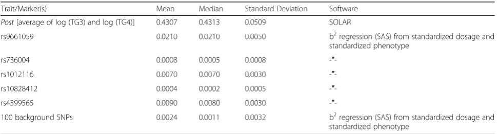
Table 1Heritability estimates of traitPost(using SOLAR)
Trait/Marker(s) Mean Median Standard Deviation Software
Post[average of log (TG3) and log (TG4)] 0.4307 0.4313 0.0509 SOLAR
rs9661059 0.0210 0.0210 0.0050 b2regression (SAS) from standardized dosage and standardized phenotype
rs736004 0.0008 0.0005 0.0008 -″ -rs1012116 0.0070 0.0070 0.0030 -″ -rs10828412 0.0004 0.0002 0.0005 -″ -rs4399565 0.0090 0.0080 0.0030 -″
-100 background SNPs 0.0024 0.0011 0.0032 b2regression (SAS) from standardized dosage and
standardized phenotype
In addition, heritabilities were estimated at 2 levels: at the full polygenic model using SOLAR (Sequential Oligogenic Linkage Analysis Routines) software [8] (http://solar-eclipse-genetics.org/) and at the single SNP level, in this case squaring beta coefficient for SNP (where using standardized dosages versus stan-dardized residuals of a normally distributed response variable after adjusting for covariates. The b2 in this case provides an approximate estimate of additive effect) [9].
To obtain an empirical null distribution for Methods I and II, we identified 2267 SNP–CpG pairs on chromo-somes 21 and 22, where there were no simulated causa-tive SNPs. A pair of markers was identified by selecting a SNP, and a CpG that is adjacent but has a higher base-pair position than the SNP. For chromosome 21, we formed 817 pairs from 10,385 SNPs and 4157 CpG sites. For chromosome 22, we formed 1450 pairs from 9464 SNPs and 8381 CpG sites.
Results
Testing ofPost(used in models 1a and 1b) for 200 replica-tions, indicated a heritability of 43% (Table1). Examination of the traits distributions after log transformation suggested the normal error assumption is not unreasonable and use of linear regressive methods appropriate.
The power to detect causative SNP by methylation inter-actions was modest to good with Methods I and II (Table2). The full GLM model (model 1a and Method I) gave power ranging from 0.91 down to 0.20 withα= 0.05 for detecting the SNP by methylation interaction at the 5 primary causa-tive sites (Table 2). The reduced GLM model, which we thought might perform better from having fewer terms, had lower power for some sites and higher power for others, depending on the strengths of the effects and the levels of methylation at each site. The very-small-effect
“background”sites were slightly better detected by the re-duced model (0.07 vs 0.06 for the full model), but power was very poor in both cases for these tiny, but real, effects. Table 2Proportion of tests withp< 0.05 under several models withproc GLMandproc MIXED
Number of tests GLM model 1a GLM model 1b MIXED model 1a MIXED model 1b MIXED model 2a MIXED model 2b cg0000036 * rs9661059 200 0.91 0.41 0.95 0.64 0.86 0.11
cg0004591 * rs1082841 200 0.20 0.28 0.28 0.40 0.29 0.06 cg0124267 * rs4399565 200 0.52 0.62 0.59 0.72 0.44 0.19 cg1048095 * rs736004 200 0.63 0.18 0.69 0.28 0.66 0.05 cg1877239 * rs1012116 200 0.78 0.45 0.83 0.62 0.74 0.12 Background SNPs 20,000 0.06 0.07 0.05 0.12 0.05 0.04 Null SNP interactions 453,400 0.05 0.05 0.05 0.05 0.05 0.05 Null SNP interactions
(w/MAC > 50)
380,800 0.05 0.05 0.05 0.05 0.04 0.04
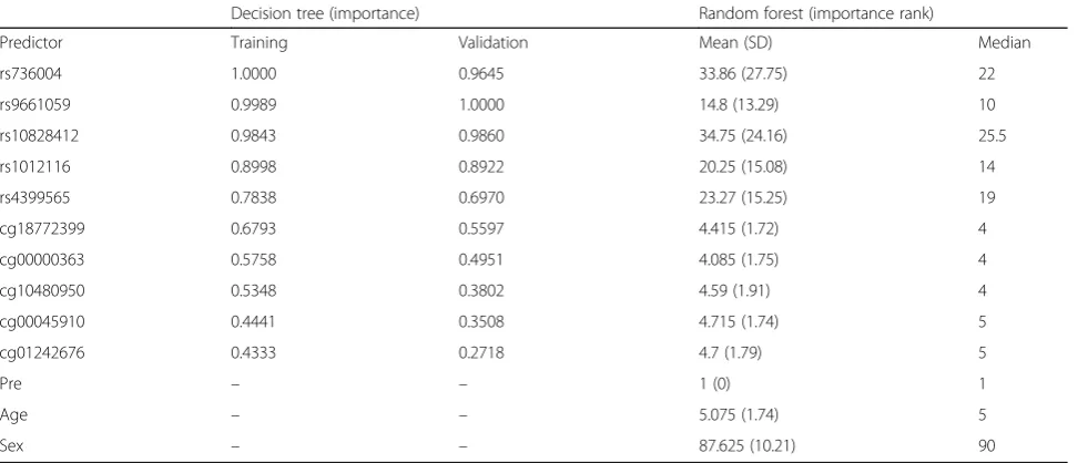
Table 3Results from decision tree analysis onPost
Decision tree (importance) Random forest (importance rank)
Predictor Training Validation Mean (SD) Median rs736004 1.0000 0.9645 33.86 (27.75) 22 rs9661059 0.9989 1.0000 14.8 (13.29) 10 rs10828412 0.9843 0.9860 34.75 (24.16) 25.5 rs1012116 0.8998 0.8922 20.25 (15.08) 14 rs4399565 0.7838 0.6970 23.27 (15.25) 19 cg18772399 0.6793 0.5597 4.415 (1.72) 4 cg00000363 0.5758 0.4951 4.085 (1.75) 4 cg10480950 0.5348 0.3802 4.59 (1.91) 4 cg00045910 0.4441 0.3508 4.715 (1.74) 5 cg01242676 0.4333 0.2718 4.7 (1.79) 5
Pre – – 1 (0) 1
Age – – 5.075 (1.74) 5
Sex – – 87.625 (10.21) 90
The full mixed model (model 1a and Method II) also showed modest to good power to detect causative SNP– CpG pairs: 0.95 down to 0.28 for the 5 main sites, and the power at each site was slightly better than for the full GLM model. The reduced mixed model (model 1b and Method II) showed better power at some sites and worse power at others, in the same directions as Method I. The detection of the“background”sites was best with the reduced mixed model, at 0.12, but in the full mixed model, this detection was no better than the null. In addition to the generating model, with the mixed model we also tested change be-tween simulated log (TG) at times 3 and 4 versus times 1 and 2 with effects from methylation level change from time 4 versus time 2 (models 2a and 2b with Method II). We see a small loss of power for this full model (2a) vs. the full gen-erating model (1a), with power from 0.86 to 0.29 at the 5 main sites for this model. However, there is a substantial loss of power in the reduced model (power ranging from 0.19 down to 0.05). This may suggest caution is required in applying the reduced model in situations where the mech-anism is not well understood. In such situations, it may be prudent to apply the full model.
Thepvalues at for the“null”sites on chromosomes 21 and 22 were distributed more or less as expected with Type I error of 0.04 to 0.05, close to nominal α= 0.05, under Methods I and II (see Table 2). However, some caution should be noted here. In an initial run (data not shown), we inadvertently used the sandwich estimator, which produced inflated p values with low minor allele frequency SNPs.
Finally, we used regression tree models (Methods III and IV) as an alternative to linear models. Table3shows the results of these methods. Individual regression trees have good performance in scenarios with large sample sizes and fewer predictors. The regression tree results represent a tree trained on all 200 replications combined (n= 136,000). In the combined data, the major known simulated SNP and CpG markers had the highest im-portance values. Conversely, random forests show high performance in scenarios with more weak predictors, but not necessarily a large sample size. We tested the relative importance of the major predictors in a random forest model (Method IV) for each replicate, and in-cluded background SNPs as superfluous predictor vari-ables. After covariates, the CpG sites reliably achieved the highest importance scores, while the SNPs that they modified had lower importance.
Discussion and conclusions
The heritability estimated reported suggested the simu-lated phenotypes had a good inheritance pattern, making it possible to detect causative SNPs and SNP–CpG inter-actions in our analyses. In examining the frequency of tests withpvalue of interactions≤0.05 in 4 models with
mixed model analysis (models 1a, 1b, 2a, and 2b for Method II; see Table2) and 2 models with GLM analysis (models 1a and 1b for Method I; see Table 2), we see reasonable power to detect these effects in this sample. When the exact mechanism is unknown, the results from models 2a and 2b suggest it may be prudent to use a full model with both main and interaction terms, but when the mechanism is well understood, neither the full model (1a) nor the reduced model (1b) was always ad-vantageous. Larger samples are required to detect these effects with these methods after correction for multiple testing. However, these results suggest that, given a suffi-cient sample, it is possible to detect gene by methylation interactions with the methods used here.
Funding
Publication of this article was supported by NIH R01 GM031575 and this study was funded in part by NHLBI R01 HL091357, NHLBI R01 HL104135, NHLBI R01 HL117078, and NIA U01 AG023746.
Availability of data and materials
The data that support the findings of this study are available from the Genetic Analysis Workshop (GAW), but restrictions apply to the availability of these data, which were used under license for the current study. Qualified researchers may request these data directly from GAW.
About this supplement
This article has been published as part of BMC Proceedings Volume 12 Supplement 9, 2018: Genetic Analysis Workshop 20: envisioning the future of statistical genetics by exploring methods for epigenetic and
pharmacogenomic data. The full contents of the supplement are available online at https://bmcproc.biomedcentral.com/articles/supplements/volume-12-supplement-9.
Authors’contributions
EWD, JH and ATK conceptualized the study, performed analyses, and drafted the manuscript; PL, SJL, JW and CW performed analyses and drafted tables for the manuscript; PA and MAP discussed the study and provided feedback; all authors read and approved the manuscript.
Ethics approval and consent to participate
Not applicable.
Consent for publication
Not applicable.
Competing interests
The authors declare that they have no competing interests.
Publisher’s Note
Springer Nature remains neutral with regard to jurisdictional claims in published maps and institutional affiliations.
Published: 17 September 2018
References
1. Jones PA. Functions of DNA methylation: islands, start sites, gene bodies and beyond. Nat Rev Genet. 2012;13:484–92.
2. Wu H, Zhang Y. Reversing DNA methylation: mechanisms, genomics, and biological functions. Cell. 2014;156:45–68.
4. Kim K, Timm NH, Timm NH. Univariate and multivariate general linear models: theory and applications with SAS. Boca Raton: Chapman & Hall/ CRC; 2007. p. xvii.
5. Littell RC. SAS System for Mixed Models. Cary: SAS Institute; 1996. 6. Matignon R. SAS Institute: Data Mining Using SAS Enterprise Miner.
Hoboken: Wiley-Interscience; 2007. p. xiii.
7. Géron A. Hands-on Machine Learning with Scikit-Learn and TensorFlow: Concepts, Tools, and Techniques to Build Intelligent Systems. Sebastopol: O’Reilly Media; 2017.
8. Almasy L, Blangero J. Multipoint quantitative-trait linkage analysis in general pedigrees. Am J Hum Genet. 1998;62:1198–211.