Training Non-Parametric Features for Statistical Machine Translation
Patrick Nguyen, Milind Mahajan and Xiaodong He Microsoft Corporation
1 Microsoft Way, Redmond, WA 98052
{panguyen,milindm,xiaohe}@microsoft.com
Abstract
Modern statistical machine translation sys-tems may be seen as using two components: feature extraction, that summarizes informa-tion about the translainforma-tion, and a log-linear framework to combine features. In this pa-per, we propose to relax the linearity con-straints on the combination, and hence relax-ing constraints of monotonicity and indepen-dence of feature functions. We expand fea-tures into a non-parametric, non-linear, and high-dimensional space. We extend empir-ical Bayes reward training of model param-eters to meta paramparam-eters of feature genera-tion. In effect, this allows us to trade away some human expert feature design for data. Preliminary results on a standard task show an encouraging improvement.
1 Introduction
In recent years, statistical machine translation have experienced a quantum leap in quality thanks to au-tomatic evaluation (Papineni et al., 2002) and error-based optimization (Och, 2003). The conditional log-linear feature combination framework (Berger, Della Pietra and Della Pietra, 1996) is remarkably simple and effective in practice. Therefore, re-cent efforts (Och et al., 2004) have conre-centrated on feature design – wherein more intelligent features may be added. Because of their simplicity, how-ever, log-linear models impose some constraints on how new information may be inserted into the sys-tem to achieve the best results. In other words,
new information needs to be parameterized care-fully into one or more real valued feature functions. Therefore, that requires some human knowledge and understanding. When not readily available, this is typically replaced with painstaking experimenta-tion. We propose to replace that step with automatic training of non-parametric agnostic features instead, hopefully relieving the burden of finding the optimal parameterization.
First, we define the model and the objective func-tion training framework, then we describe our new non-parametric features.
2 Model
In this section, we describe the general log-linear model used for statistical machine translation, as well as a training objective function and algorithm.
The goal is to translate a French (source) sentence indexed byt, with surface stringft. Among a set of
Kt outcomes, we denote an English (target) a
hy-pothesis with surface stringe(t)k indexed byk.
2.1 Log-linear Model
The prevalent translation model in modern systems is a conditional log-linear model (Och and Ney, 2002). From a hypothesis e(t)k , we extract features
h(t)k , abbreviatedhk, as a function ofe (t)
k andft. The
conditional probability of a hypothesis e(t)k given a source sentenceftis:
pk,p(e(t)k |ft),
exp[λ·hk]
Zft;λ ,
where the partition functionZft;λis given by:
Zft;λ = X
j
exp[λ·hj].
The vector of parameters of the model λ, gives a relative importance to each feature function compo-nent.
2.2 Training Criteria
In this section, we quickly review how to adjust λ to get better translation results. First, let us define the figure of merit used for evaluation of translation quality.
2.2.1 BLEU Evaluation
The BLEU score (Papineni et al., 2002) was de-fined to measure overlap between a hypothesized translation and a set of human references. n-gram overlap counts {cn}4n=1 are computed over the test
set sentences, and compared to the total counts of n-grams in the hypothesis:
cn,(t)k ,max. # of matchingn-grams for hyp.e(t)k ,
an,(t)k ,# ofn-grams in hypothesise(t)k .
Those quantities are abbreviated ck and ak to
sim-plify the notation. The precision ratio Pnfor ann
-gram ordernis:
Pn,
P
tc n,(t) k
P
ta n,(t) k
.
A brevity penalty BP is also taken into account, to avoid favoring overly short sentences:
BP,min{1; exp(1− r a)},
where r is the average length of the shortest sen-tence1, and a is the average length of hypotheses. The BLEU score the set of hypotheses{e(t)k }is:
B({e(t)k }),BP·exp 4
X
n=1 1 4logPn
.
1As implemented by NISTmteval-v11b.pl.
Oracle BLEU hypothesis: There is no easy way to pick the set hypotheses from an n-best list that will maximize the overall BLEU score. Instead, to compute oracle BLEU hypotheses, we chose, for each sentence independently, the hypothesis with the highest BLEU score computed for a sentence itself. We believe that it is a relatively tight lower bound and equal for practical purposes to the true oracle BLEU.
2.2.2 Maximum Likelihood
Used in earlier models (Och and Ney, 2002), the likelihood criterion is defined as the likelihood of an oracle hypothesis e(t)k∗, typically a single reference
translation, or alternatively the closest match which was decoded. When the model is correct and infi-nite amounts of data are available, this method will converge to the Bayes error (minimum achievable error), where we define a classification task of se-lectingk∗ against all others.
2.2.3 Regularization Schemes
One can convert a maximum likelihood problem into maximum a posteriori using Bayes’ rule:
arg max λ
Y
t
p(λ|{e(t)k , ft}) = arg max λ
Y
t
pkp0(λ),
where p0(·) is the prior distribution of λ. The
most frequently used prior in practice is the normal prior (Chen and Rosenfeld, 2000):
logp0(λ),−
||λ||2
2σ2 −log|σ|,
whereσ2 > 0is the variance. It can be thought of
as the inverse of a Lagrange multiplier when work-ing with constrained optimization on the Euclidean norm of λ. When not interpolated with the likeli-hood, the prior can be thought of as a penalty term. The entropy penalty may also be used:
H ,−1 T
T
X
t=1 Kt X
k=1
pklogpk.
2.2.4 Minimum Error Rate Training
A good way of trainingλis to minimize empirical top-1 error on training data (Och, 2003). Compared to maximum-likelihood, we now give partial credit for sentences which are only partially correct. The criterion is:
arg max λ
X
t
B({e(t)ˆ
k }) :e (t) ˆ
k = arg max e(jt)
pj.
We optimize the λ so that the BLEU score of the most likely hypotheses is improved. For that reason, we call this criterion BLEU max. This function is not convex and there is no known exact efficient op-timization for it. However, there exists a linear-time algorithm for exact line search against that objec-tive. The method is often used in conjunction with coordinate projection to great success.
2.2.5 Maximum Empirical Bayes Reward
The algorithm may be improved by giving partial credit for confidencepkof the model to partially
cor-rect hypotheses outside of the most likely hypothe-sis (Smith and Eisner, 2006):
1
T
T
X
t=1 Kt X
k=1
pklogB({ek(t)}).
Instead of the BLEU score, we use its logrithm, be-cause we think it is exponentially hard to improve BLEU. This model is equivalent to the previous model when pk give all the probability mass to the
top-1. That can be reached, for instance, when λ has a very large norm. There is no known method to train against this objective directly, however, ef-ficient approximations have been developed. Again, it is not convex.
It is hoped that this criterion is better suited for high-dimensional feature spaces. That is our main motivation for using this objective function through-out this paper. With baseline features and on our data set, this criterion also seemed to lead to results similar to Minimum Error Rate Training.
We can normalize B to a probability measure b({e(t)k }). The empirical Bayes reward also coin-cides with a divergenceD(p||b).
2.3 Training Algorithm
We train our model using a gradient ascent method over an approximation of the empirical Bayes re-ward function.
2.3.1 Approximation
Because the empirical Bayes reward is defined over a set of sentences, it may not be decomposed sentence by sentence. This is computationally bur-densome. Its sufficient statistics are r, P
tck and
P
tak. The function may be reconstructed in a
first-order approximation with respect to each of these statistics. In practice this has the effect of commut-ing the expectation inside of the functional, and for that reason we call this criterion BLEU soft. This ap-proximation is called linearization (Smith and Eis-ner, 2006). We used a first-order approximation for speed, and ease of interpretation of the derivations. The new objective function is:
J ,log ¯BP+
4
X
n=1 1 4log
P
tEc n,(t) k
P
tEa n,(t) k
,
where the average bleu penalty is:
log ¯BP,min{0; 1− r
Ek,ta1,(t)k
}.
The expectation is understood to be under the cur-rent estimate of our log-linear model. BecauseBP¯ is
not differentiable, we replace the hard min function with a sigmoid, yielding:
log ¯BP≈u(r−Ek,ta1,(t)k ) 1−
r
Ek,ta1,(t)k
! ,
with the sigmoid function u(x) defines a soft step function:
u(x), 1 1 +e−τ x,
with a parameterτ ≫1.
2.3.2 Gradients and Sufficient Statistics
We can obtain the gradients of the objective func-tion using the chain rule by first differentiating with respect to the probability. First, let us decompose the log-precision of the expected counts:
log ˜Pn= logEcn,(t)k −logEa n,(t)
Each n-gram precision may be treated separately. For eachn-gram order, let us define sufficient statis-ticsψfor the precision:
ψλc ,X
t,k
(∇λpk)ck; ψaλ,
X
t,k
(∇λpk)ak,
where the gradient of the probabilities is given by:
∇λpk=pk(hk−h¯),
with:
¯
h,
Kt X
j=1
pjhj.
The derivative of the precisionP˜nis:
∇λlog ˜Pn= 1
T
ψc λ
Eck
− ψ
a λ
Eak
For the length, the derivative oflog ¯BPis:
u(r−Ea)
(r
a−1)[1−u(r−Ea)]τ + r
(Ea)2
ψa1
λ ,
whereψa1
λ is the1-gram component ofψλa. Finally,
the derivative of the entropy is:
∇λH =
X
k,t
(1 + logpk)∇λpk.
2.3.3 RProp
For all our experiments, we chose RProp (Ried-miller and Braun, 1992) as the gradient ascent al-gorithm. Unlike other gradient algorithms, it is only based on the sign of the gradient components at each iteration. It is relatively robust to the objective func-tion, requires little memory, does not require meta parameters to be tuned, and is simple to implement. On the other hand, it typically requires more iter-ations than stochastic gradient (Kushner and Yin, 1997) or L-BFGS (Nocedal and Wright, 1999).
Using fairly conservative stopping criteria, we ob-served that RProp was about 6 times faster than Min-imum Error Rate Training.
3 Adding Features
The log-linear model is relatively simple, and is usu-ally found to yield good performance in practice. With these considerations in mind, feature engineer-ing is an active area of research (Och et al., 2004).
Because the model is fairly simple, some of the in-telligence must be shifted to feature design. After having decided what new information should go in the overall score, there is an extra effort involved in expressing or parameterizing features in a way which will be easiest for the model learn. Experi-mentation is usually required to find the best config-uration.
By adding non-parametric features, we propose to mitigate the parameterization problem. We will not add new information, but rather, propose a way to insulate research from the parameterization. The system should perform equivalently invariant of any continuous invertible transformation of the original input.
3.1 Existing Features
The baseline system is a syntax based machine translation system as described in (Quirk, Menezes and Cherry, 2005). Our existing feature set includes 11 features, among which the following:
• Target hypothesis word count.
• Treelet count used to construct the candidate.
• Target language models, based on the Giga-word corpus (5-gram) and target side of parallel training data (3-gram).
• Order models, which assign a probability to the position of each target node relative to its head.
• Treelet translation model.
• Dependency-based bigram language models.
3.2 Re-ranking Framework
Our algorithm works in a re-ranking framework. In particular, we are adding features which are not causal or additive. Features for a hypothesis may not be accumulating by looking at the English (tar-get) surface string words from the left to the right and adding a contribution per word. Word count, for instance, is causal and additive. This property is typically required for efficient first-pass decod-ing. Instead, we look at a hypothesis sentence as a whole. Furthermore, we assume that theKt-best list
In particular, the computation of the partition func-tion is performed over allKt-best hypotheses. This
is clearly not correct, and is the subject of further study. We use then-best generation scheme inter-leaved with λ optimization as described in (Och, 2003).
3.3 Issues with Parameterization
As alluded to earlier, when designing a new feature in the log-linear model, one has to be careful to find the best embodiment. In general, a set of features must satisfy the following properties, ranked from strict to lax:
• Linearity (warping)
• Monotonicity
• Independence (conjunction)
Firstly, a feature should be linearly correlated with performance. There should be no region were it matters less than other regions. For instance, in-stead of a word count, one might consider adding its logarithm instead. Secondly, the “goodness” of a hypothesis associated with a feature must be mono-tonic. For instance, using the signed difference be-tween word count in the French (source) and En-glish (target) does not satisfy this. (In that case, one would use the absolute value instead.) Lastly, there should be no inter-dependence between features. As an example, we can consider adding multiple lan-guage model scores. Whether we should consider ratios those of, globally linearly or log-linearly in-terpolating them, is open to debate. When features interact across dimensions, it becomes unclear what the best embodiment should be.
3.4 Non-parametric Features
A generic solution may be sought in non-parametric processing. Our method can be derived from a quan-tized Parzen estimate of the feature density function.
3.4.1 Parzen Window
The Parzen window is an early empirical kernel method (Duda and Hart, 1973). For an observation hm, we extrapolate probability mass around it with
a smoothing windowΦ(·). The density function is:
p(h) = 1
M
K
X
m=1
Φ(h−hm),
assuming Φ(·) is a density function. Parzen win-dows converge to the true density estimate, albeit slowly, under weak assumptions.
3.4.2 Bin Features
One popular way of using continuous features in log-linear models is to convert a single continuous feature into multiple “bin” features. Each bin feature is defined as the indicator function of whether the original continuous feature was in a certain range. The bins were selected so that each bin collects an equal share of the probability mass. This is equiva-lent to the maximum likelihood estimate of the den-sity function subject to a fixed number of rectangular density kernels. Since that mapping is not differen-tiable with respect to the original features, one may use sigmoids to soften the boundaries.
Bin features are useful to relax the requirements of linearity and monotonicity. However, because they work on each feature individually, they do not address the problem of inter-dependence between features.
3.4.3 Gaussian Mixture Model Features
Bin features may be generalized to multi-dimensional kernels by using a Gaussian smoothing window instead of a rectangular window. The direct analogy is vector quantization. The idea is to weight specific regions of the feature space differently. As-suming that we haveM Gaussians each with mean vectorµm and diagonal covariance matrixCm, and
prior weightwm. We will addmnew features, each
defined as the posterior in the mixture model:
hm,
wmN(h;µm, Cm)
P
rwrN(h;µr, Cr)
.
It is believed that any reasonable choice of kernels will yield roughly equivalent results (Povey et al., 2004), if the amount of training data and the number of kernels are both sufficiently large. We show two methods for obtaining clusters. In contrast with bins, lossless representation becomes rapidly impossible.
expectation-maximization framework (Rabiner and Huang, 1993). The number of Gaussians is typically increased exponentially.
Perceptron kernels: We also experimented with another quicker way of obtaining kernels. We chose an equal prior and a global covariance matrix. Means were obtained as follows: for each sentence in the training set, if the top-1 candidate was differ-ent from the approximate maximum oracle BLEU hypothesis, both were inserted. It is a quick way to bootstrap and may reach the oracle BLEU score quickly.
In the limit, GMMs will converge to the oracle BLEU. In the next section, we show how to re-estimate these kernels if needed.
3.5 Re-estimation Formulæ
Features may also be trained using the same empir-ical maximum Bayes reward. Let θ be the hyper-parameter vector used to generate features. In the case of language models, for instance, this could be backoff weights. Let us further assume that the fea-ture values are differentiable with respect toθ. Gra-dient ascent may be applied again but this time with respect toθ. Using the chain rule:
∇θJ = (∇θh)(∇hpk)(∇pkJ),
with∇hpk=pk(1−pk)λ. Let us take the example
of re-estimating the mean of a Gaussian kernelµm:
∇µmhm =−wmhm(1−hm)C−
1
m (µm−h),
for its own feature, and for other posteriorsr 6=m:
∇µmhr=−wrhrhmC−
1
m (µm−h),
which is typically close to zero if no two Gaussians fire simultaneously.
4 Experimental Results
For our experiments, we used the standard NIST MT-02 data set to evaluate our system.
4.1 NIST System
A relatively simple baseline was used for our exper-iments. The system is syntactically-driven (Quirk, Menezes and Cherry, 2005). The system was trained
on 175k sentences which were selected from the NIST training data (NIST, 2006) to cover words in source language sentences of the MT02 develop-ment and evaluation sets. The 5-gram target lan-guage model was trained on the Gigaword mono-lingual data using absolute discounting smoothing. In a single decoding, the system generated 1000 hy-potheses per sentence whenever possible.
4.2 Leave-one-out Training
In order to have enough data for training, we gen-erated our n-best lists using 10-fold leave-one-out training: base feature extraction models were trained on 9/10th of the data, then used for decoding the
held-out set. The process was repeated for all 10 parts. A single λwas then optimized on the com-bined lists of all systems. Thatλwas used for an-other round of 10 decodings. The process was re-peated until it reached convergence after 7 iterations. Each decoding generated about 100 hypotheses, and there was relatively little overlap across decodings. Therefore, there were about 1M hypotheses in total. The combined list of all iterations was used for all subsequent experiments of feature expansion.
4.3 BLEU Training Results
We tried training systems under the empirical Bayes reward criterion, and appending either bin or GMM features. We will find that bin features are es-sentially ineffective while GMM features show a modest improvement. We did not retrain hyper-parameters.
4.3.1 Convexity of the Empirical Bayes Reward
that this does not seriously affect the BLEU score. This is not definitive evidence but we provisionally pretend that the cost surface is almost convex for practical purposes.
24.8 24.9 25 25.1 25.2 25.3 25.4 0
200 400 600 800
BLEU score
[image:7.612.72.265.130.278.2]number of trained models
Figure 1: Histogram of BLEU scores after training from211initializations.
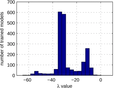
−60 −40 −20 0
0 100 200 300 400 500 600 700
λ value
number of trained models
Figure 2: Histogram of oneλparameter after train-ing from211initializations.
4.3.2 Bin Features
A log-linear model can be converted into a bin feature model nearly exactly by setting λ values in such a way that scores will be equal. Equiva-lent weights (marked as ‘original’ in Figure 3) have the shape of an error function (erf): this is because the input feature is a cummulative random variable, which quickly converges to a Gaussian (by the cen-tral limit theorem). After training theλweights for the log-linear model, weights may be converted into
bins and re-trained. On Figure 3, we show that relax-ing the monotonicity constraint leads to rough val-ues for λ. Surprisingly, the BLEU score and ob-jective on the training set only increases marginally. Starting fromλ= 0, we obtained nearly exactly the same training objective value. By varying the num-ber of bins (20-50), we observed similar behavior as well.
0 10 20 30 40 50
−1.5 −1 −0.5 0 0.5 1
bin id
value
[image:7.612.315.511.180.329.2]original weights trained weights
Figure 3: Values before and after training bin fea-tures. Monotonicity constraint has been relaxed. BLEU score is virtually unchanged.
4.3.3 GMM Features
[image:7.612.74.267.354.503.2]all additional weights set to zero, and then trained with about 50 iterations, but convergence in BLEU score, empirical reward, and development BLEU score occurred after about 30 iterations. In that set-ting, we found that regularized empirical Bayes re-ward, BLEU score on training data, and BLEU score on development and evaluation to be well corre-lated. Cursory experiments revealed that using mul-tiple initializations did not significantly alter the fi-nal BLEU score.
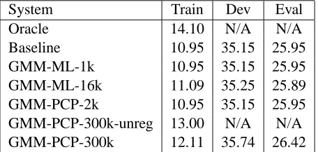
System Train Dev Eval
Oracle 14.10 N/A N/A
[image:8.612.72.300.201.310.2]Baseline 10.95 35.15 25.95 GMM-ML-1k 10.95 35.15 25.95 GMM-ML-16k 11.09 35.25 25.89 GMM-PCP-2k 10.95 35.15 25.95 GMM-PCP-300k-unreg 13.00 N/A N/A GMM-PCP-300k 12.11 35.74 26.42
Table 1: BLEU scores for GMM features vs the lin-ear baseline, using different selection methods and number of kernels.
Perceptron kernels based on the training set im-proved the baseline by 0.5 BLEU points. We mea-sured significance with the Wilcoxon signed rank test, by batching 10 sentences at a time to produce an observation. The difference was found to be sig-nificant at a 0.9-confidence level. The improvement may be limited due to local optima or the fact that original feature are well-suited for log-linear mod-els.
5 Conclusion
In this paper, we have introduced a non-parametric feature expansion, which guarantees invariance to the specific embodiment of the original features. Feature generation models, including feature ex-pansion, may be trained using maximum regular-ized empirical Bayes reward. This may be used as an end-to-end framework to train all parameters of the machine translation system. Experimentally, we found that Gaussian mixture model (GMM) features yielded a 0.5 BLEU improvement.
Although this is an encouraging result, further study is required on hyper-parameter re-estimation, presence of local optima, use of complex original
features to test the effectiveness of the parameteri-zation invariance, and evaluation on a more compet-itive baseline.
References
K. Papineni, S. Roukos, T. Ward, W.-J. Zhu. 2002.
BLEU: a method for automatic evaluation of machine translation. ACL’02.
A. Berger, S. Della Pietra, and V. Della Pietra. 1996.
A Maximum Entropy Approach to Natural Language Processing. Computational Linguistics, vol 22:1, pp.
39–71.
S. Chen and R. Rosenfeld. 2000. A survey of smoothing
techniques for ME models. IEEE Trans. on Speech and
Audio Processing, vol 8:2, pp. 37–50.
R. O. Duda and P. E. Hart. 1973. Pattern Classification
and Scene Analysis. Wiley & Sons, 1973.
H. J. Kushner and G. G. Yin. 1997. Stochastic
Approxi-mation Algorithms and Applications. Springer-Verlag,
1997.
National Institute of Standards and Technology. 2006.
The 2006 Machine Translation Evaluation Plan.
J. Nocedal and S. J. Wright. 1999. Numerical
Optimiza-tion. Springer-Verlag, 1999.
F. J. Och. 2003. Minimum Error Rate Training in
Statis-tical Machine Translation. ACL’03.
F. J. Och, D. Gildea, S. Khudanpur, A. Sarkar, K. Ya-mada, A. Fraser, S. Kumar, L. Shen, D. Smith, K. Eng, V. Jain, Z. Jin, and D. Radev. 2004. A
Smorgas-bord of Features for Statistical Machine Translation.
HLT/NAACL’04.
F. J. Och and H. Ney. 2002. Discriminative Training
and Maximum Entropy Models for Statistical Machine Translation. ACL’02.
D. Povey, B. Kingsbury, L. Mangu, G. Saon, H. Soltau and G. Zweig. 2004. fMPE: Discriminatively trained
features for speech recognition. RT’04 Meeting.
C. Quirk, A. Menezes and C. Cherry. 2005. De-pendency Tree Translation: Syntactically Informed Phrasal SMT. ACL’05.
L. R. Rabiner and B.-H. Huang. 1993. Fundamentals of
Speech Recognition. Prentice Hall.
M. Riedmiller and H. Braun. 1992. RPROP: A Fast
Adaptive Learning Algorithm. Proc. of ISCIS VII.