School of Civil and Mechanical Engineering Department of Civil Engineering
River Flow Forecasting Using an Integrated Approach of Wavelet Multi-Resolution Analysis and Computational Intelligence Techniques
Honey Badrzadeh
This thesis is presented for the Degree of Doctor of Philosophy
of Curtin University
ii
To the best of my knowledge and belief, this thesis contains no material previously published by any other person except where due acknowledgment has been made. This thesis contains no material which has been accepted for the award of any other degree or diploma in any university.
Signature:
Honey Badrzadeh Date: September 2014
iii
ABSTRACT
Reliable river flow forecasting is a key element in achieving sustainable water resources and environmental management. Accurate short term and long term river flow forecasts are particularly essential for the design of hydraulic structures, flood and drought analysis, irrigation scheduling, reservoir operation and environmental planning. Due to stochastic characteristics of hydrological events, forecasting the future condition of surface water is always associated with uncertainty. A large number of modelling techniques, ranging from physically-based to data-driven approach, have been studied to alleviate this uncertainty. As a result of technological advances in the recent years, computational intelligence approaches (CI) have become increasingly popular in hydrological modelling. Compared to conceptual and physics-based methods, CI models require minimum observation data to simulate complex hydrological processes.
This thesis focuses on improving the accuracy and reliability of river flow forecasting. Developing hybrid CI models, wavelet multi-resolution analysis is applied in conjunction with computational intelligence techniques. Two promising data-driven approaches of artificial neural networks (ANN) and adaptive neuro-fuzzy inference system (ANFIS) are adopted. Various types of ANN, ANFIS and hybrid wavelet models, are developed. Historical data of four Australian rivers, with different characteristics, are employed to investigate different applications of proposed approach in river flow forecasting.
Firstly, the impact of multivariate input selection on daily river flow forecasting is investigated when both rainfall and river flow historical time series are applied as inputs. Back propagation feed forward neural networks (BPFF), ANFIS with fuzzy C-mean clustering (FCM), hybrid wavelet neural networks (WNN) and wavelet neuro-fuzzy (WNFC) model are developed and applied for forecasting the flow of two different rivers of Harvey and Avon River in Western Australia. Application of different mother wavelet of Haar, Daubechies and Coiflet and different level of decomposition are studied.
iv
processing techniques (Coiflet, Haar and Daubechies discrete wavelets) are applied on mean daily, weekly and monthly river flow time series of Ellen Brook River in Western Australia. Preprocessed data are applied as the input of multi-layer back propagation neural networks and adaptive neuro-fuzzy inference system with grid partitioning.
Thirdly, the application of different CI models for forecasting multi-step ahead of daily river flow is studied and improved. Artificial neural networks, adaptive neuro-fuzzy inference system with subtractive clustering and their associated wavelet hybrid models (WNN and WNFS, respectively) are applied for 1, 2, 3, 4 and 5 days ahead forecasting in Harvey River, Western Australia. Daubechies and Symlet wavelets are used to decompose river flow and rainfall time series to different levels. Finally, developed models are applied to real time river flow forecasting for the purpose of timely flood warning. ANN, ANFIS with grid partitioning and their hybrid models, in conjunction with discrete wavelet transform, are applied for 1, 6, 12, 24, 36 and 48 hour ahead river flow forecasting. Casino gauging station of Richmond River, NSW, Australia, which is highly prone to flooding, is considered as the case study. The accuracy of forecasting is further improved when an upstream river flow data (Wiangaree station), are employed as additional input.
In each case study, optimum structure of different CI models is determined and the best fitted model among all is selected. The outcomes of this study confirm the robustness of CI models in river flow forecasting. Considering highly nonlinear and non-stationary characteristics of river flow time series, wavelet analysis significantly improved forecasting reliability in the proposed hybrid models, especially for longer lead time and higher step ahead forecasting. Moreover, hybrid models are highly outperform classical CI models in forecasting sudden extreme events. The outcome of this study will assist hydrologists and decision makers in forecasting river flows and sustainable planning and management of water resources.
v
I would like to take this opportunity to express my sincere gratitude to my supervisor, Dr. Rnajan Sarukkalige, for his continuous guidance and encouragement throughout this study. Without his advice and active support, this project would not have been possible. My appreciation is also extended to my co-supervisor Prof. Amithirigala Jayawardena for his enormous knowledge, invaluable guidance and advice.
I would like to acknowledge Department of Civil Engineering of Curtin University for providing all sorts of support in conducting this research. I also would like to give my special thanks to Prof. Hamid Nikraz, former head of the department and member of thesis committee, for his endless support and encouragement.
Last but not least, I would like to thank my family members, especially my father and brother, my dearest friends, Bahar Baniahmad and Kaveh Espandar, for their permanent encouragement, understanding and generous support during my PhD study. I would like to extend my special thanks to my fiancé, Dr. Meysam Banimahd, for his ongoing support, valuable comments and editing the thesis.
vi
Articles in Journals
• Badrzadeh, H., Sarukkalige, R., & Jayawardena, A. W. (2013). Impact of multi-resolution analysis of artificial intelligence models inputs on multi-step ahead river flow forecasting. Journal of Hydrology, 507(0), 75-85.
doi: http://dx.doi.org/10.1016/j.jhydrol.2013.10.017
• Badrzadeh, H., Sarukkalige, R. & Jayawardena, A. W. (2014). Improving ANN-based short and long term seasonal river flow forecasting with signal processing techniques, River research and application journal, doi: 10.1002/rra.2865.
• Badrzadeh, H., Sarukkalige, R. & Jayawardena, A. W. (2015). A wavelet neuro-fuzzy computational model for stream flow forecasting, Nonlinear
processes in geophysics, Under review.
Articles in peer reviewed conference proceedings
• Badrzadeh, H. & Sarukkalige, R. (2012) River flow forecasting using an integrated approach of wavelet analysis and artificial neural networks, in
Proceedings of the 34th Hydrology & Water Resources Symposium, Nov
19-22 2012, pp. 1571-1578. Sydney, NSW: Engineers Australia.
• Badrzadeh, H., Sarukkalige, R. & Jayawardena, A. W. (2012) Combined wavelet-neural network model for intermittent stream flow prediction, in Vimonsatit, V. and Singh, A. and Yazdani, S., Research, Development, and
Practice in Structural Engineering and Construction, Nov 28-Dec 2 2012,
pp. 769-774. Perth, Western Australia.
• Badrzadeh, H. & Sarukkalige, R. (2014) Improving fuzzy-based model for seasonal river flow forecasting, in Proceedings of the 35th Hydrology &
Water Resources Symposium, Feb 24-27 2014, pp. 994-1001. Perth, WA:
vii
Declaration ... ii Abstract ... iii Acknowledgements ...v List of Publication ... vi
Table of Contents ... vii
List of Figures ... xi
List of Tables... xv
List of Acronyms ... xvii
List of Notations ...xix
Chapter 1: Research Overview ... 1
1.1 Background ...1
1.2 Motivation ...2
1.3 Thesis objective and scope ...3
1.4 Structure of the thesis...4
Chapter 2: A Review on River Flow Forecasting Methods ... 8
2.1 Introduction ...8
2.2 Physically-based models ...9
2.3 Conceptual models... 12
2.4 Data driven models ... 17
2.4.1 Classical data driven approach ... 18
2.4.2 Computational intelligence approach ... 18
Chapter 3: Computational Intelligence Approach ... 21
3.1 Introduction ... 21
3.2 Artificial Neural Networks ... 21
viii
3.2.3.1 Feed-forward multilayer perceptron ANN ... 29
3.2.4 Neural network learning ... 31
3.2.4.1 Backpropagation algorithm ... 31
3.3 Neuro-fuzzy modelling ... 35
3.3.1 Introduction ... 35
3.3.2 Fuzzy logic ... 37
3.3.3 Fuzzy inference systems ... 40
3.3.4 Adaptive neuro-fuzzy inference system ... 41
3.3.5 Input space partitioning ... 45
3.3.5.1 Grid partitioning ... 45
3.3.5.2 Scatter partitioning (Clustering) ... 45
3.4 Wavelet multi-resolution Analysis ... 49
3.4.1 Introduction ... 49
3.4.2 Fourier transform ... 51
3.4.3 Short-time fourier transform ... 51
3.4.4 Continuous wavelet transform ... 52
3.4.5 Discrete wavelet transform ... 53
3.4.6 Mother wavelets ... 54
3.4.7 Time series decomposition by wavelet ... 57
3.5 Summary ... 59
Chapter 4: Structure of Proposed Hybrid Models ... 60
4.1 Introduction ... 60
4.2 Wavelet neural networks ... 60
4.2.1 Neural networks sub-model ... 61
4.2.2 Wavelet sub-model ... 64
4.3 Wavelet neuro-fuzzy with grid partitioning ... 66
4.3.1 ANFIS sub-model with grid partitioning ... 66
4.3.2 Wavelet sub-model ... 68
4.4 Wavelet neuro-fuzzy with clustering ... 69
ix
4.5 Performance criteria ... 73
4.6 Summary ... 76
Chapter 5: Daily River Flow Forecasting Using Multivariate Inputs
... 77
5.1 Introduction ... 77
5.2 Case studies ... 78
5.3 Application of ANN... 83
5.4 Application of ANFIS ... 85
5.5 Improving the efficiency with hybrid models ... 86
5.6 Conclusion ... 93
Chapter 6: Short Term and Long Term River Flow Forecasting ... 93
6.1 Introduction ... 93
6.2 Study area and data used ... 94
6.3 Input selection for models ... 95
6.4 Results and discussion ... 100
6.4.1 Performance of ANN-based models in river flow forecasting... 100
6.4.2 Performance of Fuzzy-based models in river flow forecasting... 111
6.5 Conclusion ... 122
Chapter 7: Multi-Step Ahead River Flow Forecasting... 123
7.1 Introduction ... 123
7.2 Study area and data used ... 124
7.3 Results and discussion ... 125
7.3.1 Application of ANN ... 125
7.3.2 Improving the efficiency of ANN with WNN ... 128
7.3.3 Application of ANFIS ... 138
7.3.4 Improving the efficiency of ANFIS with WNF ... 139
7.3.5 Model comparison ... 144
x
8.1 Introduction ... 150
8.2 Study area and data used ... 151
8.3 Analysis and results ... 154
8.3.1 ANN-based models ... 154
8.3.2 Fuzzy-based models... 159
8.3.3 Models comparison ... 165
8.4 Conclusion ... 169
Chapter 9: Conclusions and Future Work ... 170
9.1 Conclusion ... 170
9.2 Recommendation for future works ... 173
xi
Figure 1. 1 Main structure of the thesis ... 7
Figure 2. 1 Schematic of MIKE SHE distributed model structure (Graham and Butts, 2005). . 11
Figure 2. 2 Schematic of storage system in conceptual model ... 13
Figure 2. 3 Learning system in black box data driven approaches. ... 17
Figure 3. 1 Schematic of a neuron function system. ... 25
Figure 3. 2 Sigmoid activation function with different steepness parameter. ... 26
Figure 3. 3 Tan-Sigmoid activation function with different steepness parameter. ... 26
Figure 3. 4 Schematic diagram of a three-layer feed-forward neural network. ... 30
Figure 3. 5 Structure of neural networks with back propagation training algorithm. ... 32
Figure 3. 6 Levenberg-Marquardt algorithm shifts from the steepest descent to the Gauss-Newton method of decreasing the value of μ . ... 34
Figure 3. 7 The basic structure of FIS. ... 40
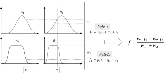
Figure 3. 8 Reasoning mechanism of a Sugeno fuzzy model with two inputs and rules. ... 43
Figure 3. 9 Equivalent ANFIS architecture for two-input first-order TSK fuzzy model with two rules. ... 43
Figure 3. 10 Grid partitioning of two inputs into 9 fuzzy rules. ... 46
Figure 3. 11 (a) Shifted and (b) Scaled wavelet illustration. ... 53
Figure 3. 12 Daubechies family wavelet. ... 55
Figure 3. 13 Haar mother wavelet function. ... 56
Figure 3. 14 Mexican Hat, Morlet, Coiflet1 and Symlet2 mother wavelets. ... 56
Figure 3. 15 Diagram of multi-resolution analysis of signal. ... 57
Figure 3. 16 Two noisy signals and their (a) Daubechies3 (b) Coiflet1 wavelet coefficients. ... 58
Figure 4. 1 Structure of the proposed hybrid WNN model for N step ahead forecasting. ... 61
Figure 4. 2 Feed-forward neural network sub-model flow chart. ... 63
Figure 4. 3 hybrid wavelet neural networks model flow chart. ... 65
Figure 4. 4 Structure of Wavelet Neuro-Fuzzy hybrid model for N step ahead forecasting. ... 66
Figure 4. 5 Adaptive neuro-fuzzy with grid partitioning sub-model flow chart. ... 67
Figure 4. 6 Flow chart of hybrid wavelet neuro-fuzzy model with grid partitioning. ... 69
Figure 4. 7 Flow chart of hybrid wavelet neuro-fuzzy model with subtractive clustering... 71
Figure 4. 8 Flow chart of hybrid wavelet neuro-fuzzy model with FCM clustering. ... 72
Figure 5. 1 Map of Northam weir and Dingo road station location in Western Australia (Bureau of meteorology, 2013) ... 80
Figure 5. 2 Daily river flow time series at the Dingo road station in the Harvey River, Western Australia (1976-2011)... 81
Figure 5. 3 Daily rainfall time series near the Dingo road station in the Harvey River, Western Australia (1976-2011)... 81
xii
Figure 5. 5 Daily rainfall time series near the Northam weir station in the Avon River, Western Australia (1978-2010)... 82 Figure 5. 6 (a) Harvy and (b) Avon River mean daily river flow hydrographs in selected years.
... 83 Figure 5. 7 Scatter plots between Dingo road station observed and modelled daily river flow: (a)
ANN single flow input; (b) ANN with multivariate input. ... 85 Figure 5. 8 Scatter plots between Northam weir station observed and modelled daily river flow: (a) ANN with single input; (b) ANN with multivariate input... 85 Figure 5. 9 Scatter plots between Dingo road station observed and modelled daily river flow
with: (a) ANN1; (b) Hybrid WNN12; (c) ANFIS1; (d) Hybrid WNFC4. ... 89 Figure 5. 10 Comparison of the Dingo road observed and predicted daily river flow with
WNN12... 91 Figure 5. 11 Comparison of the Dingo road observed and predicted daily river flow with
WNN12 in the validation set (2007-2011). ... 91 Figure 5. 12 Comparison of the Northam weir observed and predicted daily river flow with
WNN9 ... 92 Figure 5. 13 of the Northam weir observed and predicted daily river flow with WNN9 in the
validation set (2006-2010). ... 92 Figure 6. 1 Location of Ellen Brook catchment in the Western Australia. ... 94 Figure 6. 2 (a) Daily; (b) Weekly and (c) Monthly river flow time series at the Railway Parade
station on the Ellen Brook River, Western Australia (1977-2010). ... 97 Figure 6. 3 ACF of Ellen Brook River daily, weekly and monthly flow time series (1977-2010).98 Figure 6. 4 Nash-Sutcliffe coefficient of efficiency of (a) training and (b) validation set, for
different BPNN and WNN models. ... 104 Figure 6. 5 Ellen Brook weekly river flow time series and its wavelet coefficients with Coif1
wavelet. ... 105 Figure 6. 6 Scatter plots of observed and forecasted river flow with the best fitted BPNN and
WNN models for daily, weekly and monthly forecasting. ... 106 Figure 6. 7 Comparing observed versus modeled monthly river flow with best fitted BPNN
model. ... 108 Figure 6. 8 Comparing observed versus modeled monthly river flow with best fitted WNN
model. ... 108 Figure 6. 9 Comparing observed versus modeled weekly river flow with best fitted BPNN
model. ... 109 Figure 6. 10 Comparing observed versus modeled weekly river flow with best fitted WNN
model. ... 109 Figure 6. 11 Best fitted hybrid neuro-fuuzy model (WNFG-M2) structure for monthly
xiii
Figure 6. 13 Ellen Brook daily river flow signal and its wavelet coefficients with db5 wavelet. ... 116 Figure 6. 14 Scatter plots of observed and forecasted river flow with the best fitted ANFIS and
WNFG models for daily, weekly and monthly forecasting. ... 117 Figure 6. 15 Comparing observed versus modeled weekly river flow with best fitted ANFIS
model. ... 120 Figure 6. 16 Comparing observed versus modeled weekly river flow with best fitted WNFG
model. ... 120 Figure 6. 17 Comparing observed versus modeled monthly river flow with best fitted ANFIS
model. ... 121 Figure 6. 18 Comparing observed versus modeled monthly river flow with best fitted WNFG
model. ... 121 Figure 7. 1 ACF of Harvey River daily flow and rainfall time seires. ... 124 Figure 7. 2 Scatter plots of observed and ANN forecasted flow for different lead time. ... 128 Figure 7. 3 Daily river flow time series and its db5 wavelet coefficients with four level of
resulotion. ... 129 Figure 7. 4 Different hybrid WNN model efficiency for different lead-time (L) in training and
validation set. ... 135 Figure 7. 5 Best fitted ANN and WNN model efficiency (RMSE) variation over the lead time in
(a) training; (b) verification set... 136 Figure 7. 6 Comparison of the observed and modeled river flow for 5-day ahead with ANN5-5
and WNND5-14 models (1972-2011). ... 137 Figure 7. 7 Scatter plots of observed and ANFIS forecasted flow for different lead time. ... 139 Figure 7. 8 Hybrid WNFD1-1 model structure, generated with subtractive clustering approach.
... 140 Figure 7. 9 Different hybrid WNF model efficiency for different lead-time (L) in training and
validation set. ... 142 Figure 7. 10 ANFIS and WNF models’ efficiency (RMSE) variation over the lead time in (a)
training; (b) verification set. ... 142 Figure 7. 11 Comparison of the observed and modeled river flow for 5-day ahead with ANFIS5-2 and WNFD5-ANFIS5-2 models (197ANFIS5-2-ANFIS5-2011). ... 143
Figure 7. 12 Variation of different models’ performance (𝑹𝟐) over the lead time. ... 144
Figure 7. 13 Comparison of the observed and modeled river flow for 5-day ahead with best fitted WNN and WNF models (2006-2011). ... 145 Figure 7. 14 Scatter plots of five-day ahead forecasting of the best fit ANN, WNN, ANFIS and
WNF model. ... 147 Figure 7. 15 Highest observed river flow in historical time series and its estimation with
xiv
Figure 8. 2 Hourly river flow and rainfall time series of Casino station for (a) training and (b) validation set. ... 153 Figure 8. 3 Hourly river flow and rainfall time series of Wiangaree station for (a) training and
(b) validation set. ... 153 Figure 8. 4 Nash-Sutcliffe coefficient of (a) training and (b) validation set of ANN-based models. ... 157 Figure 8. 5 Root mean square error of (a) training and (b) validation set of ANN-based models.
... 157 Figure 8. 6 Scatter plots of observed and simulated river flow for 24 hour lead time with
different ANN-based models... 158 Figure 8. 7 Comparing observed flood versus ANN-based modeled hourly river flow (24 hour
ahead forecasts). ... 159 Figure 8. 8 Comparing four highest observed peak flow versus ANN-based modeled values (24
hour ahead forecasts). ... 159 Figure 8. 9 Nash-Sutcliffe coefficient of (a) training (b) validation set of fuzzy-based models. 163 Figure 8. 10 Root mean square error of (a) training and (b) validation set of fuzzy-based
models. ... 163 Figure 8. 11 Scatter plots of observed and simulated river flow for 24 hour lead time with
different fuzzy-based models. ... 164 Figure 8. 12 Comparing observed flood versus fuzzy-based modeled hourly river flow (24 hour
ahead forecasts). ... 165 Figure 8. 13 Comparing four highest observed peak flow versus fuzzy-based modeled values (24
hour ahead forecasts). ... 165 Figure 8. 14 Scatter plots of observed and simulated river flow for 12 hour lead time with best
fitted ANN, WNN, ANFIS and WNF models. ... 167 Figure 8. 15 Scatter plots of observed and simulated river flow for 24 hour lead time with best
fitted ANN, WNN, ANFIS and WNF models. ... 167 Figure 8. 16 Scatter plots of observed and simulated river flow for 36 hour lead time with best
fitted ANN, WNN, ANFIS and WNF models. ... 168 Figure 8. 17 Scatter plots of observed and simulated river flow for 48 hour lead time with best
xv
Table 3. 1 Different types of linear activation functions. ... 28
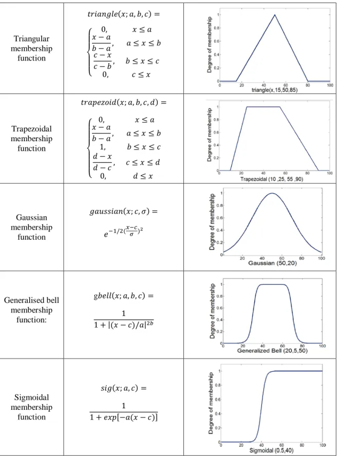
Table 3. 2 Triangular, Trapesoidal, Gaussian, Generalised bell and Sigmoidal membership functions. ... 39
Table 5. 1 Daily statistical parameters of stream flow and rainfall data sets of the Dingo road and Northam weir stations. ... 79
Table 5. 2 ANN models structure and performance. ... 84
Table 5. 3 ANFIS models’ performance. ... 86
Table 5. 4 Hybrid models’ structure and performance for Dingo road station daily river flow forecast. ... 87
Table 5. 5 Hybrid models’ structure and performance for Northam weir station daily river flow forecast. ... 88
Table 6. 1 Statistical parameters of Ellen Brook river flow data sets of the Railway parade station. ... 95
Table 6. 2 Input selection for different BPNN models. ... 98
Table 6. 3 Input selection for different ANFIS models... 99
Table 6. 4 Input pre-processing type for hybrid WNN models. ... 100
Table 6. 5 Input pre-processing type for hybrid WNFG models... 100
Table 6. 6 BPNN and WNN models structure and performance for daily river flow forecasting. ... 102
Table 6. 7 BPNN and WNN models structure and performance for weekly flow forecasting. . 102
Table 6. 8 BPNN and WNN models structure and performance for monthly flow forecasting. ... 103
Table 6. 9 Accuracy of developed ANN-based models in simulating daily, weekly and monthly extreme flow values. ... 110
Table 6. 10 ANFIS and WNFG models structure and performance for daily river flow forecasting. ... 112
Table 6. 11 ANFIS and WNFG models structure and performance for weekly river flow forecasting. ... 113
Table 6. 12 ANFIS and WNFG models structure and performance for monthly river flow forecasting. ... 113
Table 6. 13 Accuracy of developed Fuzzy-based models in simulating daily, weekly and monthly extreme flow values. ... 119
Table 7. 1 ACF of Harvey River daily flow and rainfall time series (1972-2011). ... 124
Table 7. 2 Different input combinations. ... 125
Table 7. 3 ANN structure and performance for different lead time. ... 126
Table 7. 4 Different WNN model’s structure and performance for 1 day ahead lead-time... 130
xvi
Table 7. 8 Different WNN model’s structure and performance for 5 day ahead lead-time... 134
Table 7. 9 ANFIS performance for different lead time. ... 138
Table 7. 10 WNF models' structure and performance for different lead time... 141
Table 7. 11 Best fitted models performances for different lead time. ... 146
Table 7. 12 Accuracy of different model in simulating five-day ahead extreme flow values. ... 147
Table 8. 1 Statistical parameters of Richmond River flow data sets of the Casino and Wiangaree stations... 152
Table 8. 2 ANN models structure and performance using only Casino station data. ... 154
Table 8. 3 ANN models structure and performance using Casino and Wiangaree stations data. ... 154
Table 8. 4 Hybrid WNN models structure and performance using only Casino station data. . 155
Table 8. 5 Hybrid models structure and performance using Casino and Wiangaree stations data. ... 156
Table 8. 6 ANFIS models structure and performance using only Casino station data. ... 160
Table 8. 7 ANFIS models structure and performance using Casino and Wiangaree stations data. ... 161
Table 8. 8 WNF models structure and performance using only Casino station data... 162
Table 8. 9 WNF models structure and performance using Casino and Wiangaree stations data. ... 162
xvii
A Approximation
ACF Autocorrelation function
ANFIS Adaptive neuro-fuzzy inference system
ANN Artificial neural networks
AR Autoregressive
ARIMA Autoregressive integrated moving average
ARMA Autoregressive moving average
ARX Autoregressive exogenous
B Bias
BP Back propagation algorithm
BPFF Back propagation feed-forward
BPNN Back propagation neural networks
CI Computational intelligence
Coif Coiflets wavelet
CWT Continuous wavelet transform
D Details
d Agreement index
db Daubechies wavelet
DWT Discrete wavelet transform
EPA Environmental protection agency
FCM Fuzzy C-mean clustering
FFNN Feed-forward neural networks
FIS Fuzzy inference systems
FL Fuzzy logic
FT Fourier transform
HSPF Hydrologic simulation program FORTRAN
I Identity matrix
IHDM Institute of hydrology distributed model
LM Levenberg-Marquardt algorithm
LSE Least square error
MA Moving average
MAE Mean absolute error
xviii
MLR Multiple linear regression
MRA Multi-resolution analysis
MSE Mean square error
NSE Nash-Sutcliffe coefficient of efficiency
PB Percent bias
PE Potential error
R Coefficient of correlation
R2 Coefficient of determination
RBF Radial basis function
RMAE Relative mean absolute error
RMSE Root mean square error
R-R Rainfall-runoff
RSR Root mean square error-standard deviation ration SAC-SMA Sacramento soil moisture accounting
SHE Système Hydrologique Européenne (European Hydrological System)
SMAR Soil moisture accounting and routing SMSC
SOFM
Soil moisture storage capacity Self organizing feature map
SOM Self organized map
STDV Standard deviation
STFT Short-time Fourier transform
SWM Standford watershed model
SWMM Storm water management hydrological model
SWWA South West of Western Australia
Sym Symlet wavelet
TAR Threshold autoregressive
TSK Takagi-Sugeno-Kang fuzzy
Var Variance
WNF Wavelet neuro-fuzzy
WNFC Wavelet neuro-fuzzy with C-mean clustering WNFG Wavelet neuro-fuzzy with grid partitioning WNFS Wavelet neuro-fuzzy with subtractive clustering
xix
α Weighting exponent
εt White noise
φp Autoregressive coefficient (order p)
ψ(α,β) Mother wavelet
θq Moving average coefficient (order q)
μR(x) Membership of an element 𝑥
∇V Gradient
∇2V (w) Hessian matrix
ai, bi, ci Premise parameters
pi, qi, ri Consequent parameters (polynomial parameters)
bj Threshold value (bias) of 𝑗𝑡ℎneuron
C Number of clusters
Di Density measure of 𝑖𝑡ℎ cluster centre
en Model error in 𝑛𝑡ℎ iteration
fh Hidden layer activation function
fo Output layer activation function
It Stream flow time series
J (w) Jacobian matrix
K Number of inputs
m Number of membership function
mij Membership degree of 𝑗𝑡ℎ variable in data set for 𝑖𝑡ℎ cluster
N Length of time series
Ok,i Output of 𝑖𝑡ℎ node in𝑘𝑡ℎ layer
Qt River flow time series
Qdt Daily river flow time series
Qw Weekly river flow time series
Qmt Monthly river flow time series
Qsim Simulated river flow
Qobs Observed river flow
QDWT Wavelet coefficient of river flow time series
xx
RDWT Wavelet coefficient of rainfall time series
vi Cluster centre of the 𝑖𝑡ℎ cluster
W(α,β) Scaled (α-scaled) and shifted (β-translation) wavelet coefficients
W(α,β)2 Wavelet spectrum
Wij Connection weight from the𝑖𝑡ℎ neuron to the𝑗𝑡ℎ neuron
W(t) Window function
x An input vector
xn Normalized value of x
Chapter 1
Research Overview
1.1 BACKGROUND
Water demands are increasingly growing due to population growth and irrigation and industrial developments. Surface water availability is likely to decrease as a reason of global warming, urbanizations and excessive groundwater extractions. On the other hand, in various regions around the world, extreme weather conditions resulting floods, droughts and heat waves.
Understandably, reliable information on current and future water availability is essential to properly manage the limited water resources and flood mitigation. Authorities in water sector cannot allocate water resources optimally for water demands like agricultural, industrial, domestic, hydropower generation and environmental maintenance, unless they are equipped with a reliable forecasting of river flow. Accurate forecasting of river flow, as the main part of the available water resources, is also a key element in drought analysis and design of water related infrastructures. Therefore, improving the accuracy and reliability of river flow forecasting is an ongoing research. Researchers are keen to develop and investigate various types of hydrological forecasting approaches to attain better management of scarce water resources and minimize the risk of any potential flooding.
2
1.2 MOTIVATION
Like many countries around the world, Australia is increasingly facing water scarcity. Many parts of Australia continent are in drought. South Western Austalia, in particular, is suffering from extended dry period since 1975. Climate change projections for Southern part of the continent, more populated part of Australia, indicates reduction in total rainfall and water supply (Charters and Williams, 2006). At the same time, climate change causes more frequent rainfall events with higher intensity which increases the risk of flooding (Bates et al., 2008). Undoubtedly, effective water governance policies will become critical to cope with water crises. Forecasting future surface water availability is a key element in assisting decision makers in water resources planning and management (Nash and Sutcliffe, 1970; Nayak et al., 2005; Sene, 2010; Piotrowski and Napiorkowski, 2011; Zeng et al., 2012). Forecasting water availability is always associated with large uncertainties and complexities. For example, determining the rate of runoff generated by rainfall and its routing is a very complex matter as an extensive number of parameters are involved in this process. A significant amount of research has been carried out to improve the accuracy of forecasting ranging from physically-based to data-driven approaches. Therefore, improving the accuracy of forecasting is a continuing research field as each hydrological forecasting approach has its own characteristics and limitations. This study focuses on developing river flow forecasting model with minimum parameter requirements (ungauged catchments) and maximum accuracy for long term as well as extreme event forecasting. For this research, computational intelligence (CI) approach is selected because of their cost-efficiency, accuracy and robustness.
In order to boost the forecasting performance, some hybrid approaches have been proposed recently (Sivakumar and Berndtsson, 2010). One of the recent developments in river flow forecasting is based on coupling computational intelligence models with wavelet analysis. River flow historical data are non-stationary time series with a wide range of frequency components. By applying wavelet transform, river flow complex time series can be decomposed into its major sub-components (Zhou et al., 2008). However, a comprehensive literature review
3
confirms the lack of research on wavelet neuro-fuzzy techniques with a subtractive clustering method for river flow simulation and forecasting. Furthermore, only a limited number of river discharge time series have been used for verification of the wavelet neural network based models. More data from different areas with different characteristics would be required to conclusively prove the advantages of this hybrid approach (Wei et al., 2012). Available research in the literature mainly focuses on the forecasting river flow by using only river flow discharge time series. Forecasting could be improved by adding other hydrological time series and variables which affect river flow (Adamowski and Sun, 2010; Pramanid et al., 2011). In addition, very few researchers explored the application of hybrid models on seasonal river flow forecasting and lead times of more than one day, but less than one month (Wu et al., 2009; Nournani et al., 2013).
Taking these considerations into account, this study aims at improving seasonal, short term, long term and real time river flow forecasting by various classical and hybrid computational intelligence approaches with different structures and input selections. By providing more accurate tools, the ultimate scope of this research is to assist decision makers in sustainable water resources planning, flood protection, mitigation of contamination or licensing of exploitations.
1.3 THESIS OBJECTIVE AND SCOPE
The main purpose of this research is to develop highly efficient, reliable and accurate data driven model for river flow forecasting. Each of the forecasting approaches has its own advantages and disadvantages and there is no perfect model or modelling technique to guarantee precise future long term prediction. Reviewing current available river flow forecasting and rainfall-runoff methods, computational intelligence techniques were found as a powerful approach for modelling complex hydrological process. In this study different type and structure of artificial neural networks (ANN), adaptive neuro-fuzzy inference system (ANFIS) and hybrid wavelet models will be developed. Comparing the performance of models, the best
4
fitted model for reaching the most accurate results in different study areas will be determined. In summary, the main objectives of this study are;
• Developing highly efficient model for accurate river flow forecasting by investigating and comparing the performance of artificial neural networks and adaptive neuro-fuzzy inference system approaches.
• Applying different methods for initiating fuzzy inference system (FIS) structure in ANFIS modelling, including grid partitioning, subtractive clustering and C-mean clustering (FCM).
• Finding the optimum structure and most effective training algorithm of neural network for river flow forecasting.
• Investigating the impact of wavelet multi-resolution analysis of CI model inputs on forecasting accuracy. Explore the performance of hybrid wavelet models by decomposing data series into the low and high frequency signals with different type of discrete wavelet transforms and into different level of decomposition.
• Developing and validating different computational intelligence techniques for real time, short term, long term and multi-step ahead prediction of stream flow. Also, determining and validating the best fitted CI model structure for seasonal river flow forecasting.
1.4 STRUCTURE OF THE THESIS
This thesis is designed in four main parts of introduction, methodology, applications and conclusion which are expanded in 9 chapters. Figure 1.1 depicts the structure of the thesis. Following is a brief description of each chapter;
5
Chapter One- This chapter mainly identifies the problem and the main reasons of conducting this research. It highlights the core objectives of the study and thesis outlines.
Chapter Two- This chapter introduces various types of river flow forecasting and rainfall-runoff models. Physically-based, conceptual and data-driven approaches are reviewed. Methodologies behind most popular models are briefly explained. Advantages and drawbacks of different approaches are identified.
Chapter Three- Three different CI approaches, namely, artificial neural networks, fuzzy modelling and wavelet analysis (as a part of hybrid models) are discussed in details in this chapter. The structure of feed-forward neural networks with back propagation training algorithm, adaptive neuro-fuzzy inference system with grid partitioning, subtractive and C-mean clustering is described. The application of wavelet multi-resolution analysis in signal decomposition is also presented. In addition to theoretical description of approaches, a review on their background and applications in hydrology is also provided.
Chapter Four- This chapter presents the structure of developed models, including four hybrid models of wavelet neural networks, wavelet neuro-fuzzy with grid partitioning, subtractive clustering and C-mean clustering. Optimum performance criteria are also selected for achieving most efficient models, especially for extreme event forecasting.
Chapter Five- In this chapter, application of developed models with multivariate inputs for daily river flow forecasting is investigated. Rainfall time series are added as an additional input. Two different rivers from Western Australia (Harvey and Avon Rivers) are selected as case studies. The best structure of ANN and ANFIS with C-mean clustering, alone and in conjunction with Daubechies and Haar mother wavelet (WNN, WNFC), are determined. The effect of adding an additional input is discussed.
6
Chapter Six- This chapter investigates the application of developed models in both short and long term river flow forecasting. Different input combinations (forward stepwise selection) and signal processing techniques (Coiflet, Haar and Daubechies mother wavelets) are applied on multi-layer back propagation neural networks (WNN) and adaptive neuro-fuzzy inference system with grid partitioning (WNFG). The data of the Railway parade station on Ellen Brook River, Western Australia, is used as a case study. Daily, weekly and monthly river flow forecasting is conducted. The impacts of right selection of the inputs and pre-processing the raw data with wavelet are showcased in this section.
Chapter Seven- In this chapter the accuracy of multi step ahead daily river flow forecasting is improved by applying Daubechies and Symlet multi-resolution analysis on ANN and ANFIS models’ input. A novel approach of hybrid wavelet neuro-fuzzy with subtractive clustering is introduced for river flow forecasting. Overall 215 different models for various lead-times of 1 to 5 days ahead, with different input combinations (forward stepwise time series, multivariate input and wavelet coefficients) were developed for forecasting daily river flow of the Dingo road station on Harvey River, Western Australia. Highly satisfactory results achieved as the forecasting accuracy significantly improved for longer lead time and extreme event simulation.
Chapter Eight- In this chapter the application of developed models for timely flood warning is investigated. Feed-forward ANN, adaptive neuro-fuzzy with grid partitioning alone and in conjunction with Daubechies discrete wavelet transform (db3) are applied for forecasting 1, 6, 12, 24, 36 and 48 hour ahead of river flow. Hourly rainfall and river flow data of two stations on Richmond River in NSW, Australia, which is highly prone to flooding, are used. Highly reliable results are achieved for forecasting up to 24 hour ahead of flooding event, especially when an upstream flow time series added as the model input.
7
Chapter Nine- Summary of research outcomes and general conclusions are presented in this chapter. The recommendations for future studies are also provided in this chapter.
Chapter 2
A Review on River Flow Forecasting Methods
2.1 INTRODUCTION
As a consequence of issues like water increased demands and climate change, the need for accurate river flow forecasting has grown rapidly in the past decades. Knowing future conditions of surface water resources is one of the key elements for an appropriate risk-based and sustainable water resources planning.
The application of river flow forecasting could be categorized into two main types. The first application is short term river flow forecasting to predict sudden extreme conditions such as flooding (Werner, et al., 2005; O’Connor, 2006). Being prepared a day or even a few hours before such an event could assist hazard adaptation which can reduce costs and save lives (Carpernter, et al., 1999). The second application is long term forecasting for the purpose of sustainable water resources management. Knowing the quantity of future surface water resources is required for determining optimum reservoir operations, irrigation allocations, groundwater extraction regulation and demands supply planning (Valenca, et al., 2005; Ghanbarpour et al, 2009; Sudheer, et al., 2014).
There are various types of river flow forecasting and rainfall-runoff (R-R) techniques ranging from deterministic to stochastic models (Clarke, 1973). The oldest and still the most widely-used rainfall-runoff approach is based on the rational formula (Mulaney, 1845), which estimates runoff rate from rainfall intensity and the catchment area. Technological advances have made a significant impact on
9
hydrology science in the last centuries. A growing number of scientific theories and mathematical techniques have been developed for measurements, modelling and forecasting of hydrological phenomena. Selecting the best approach for forecasting depends on the purpose of the modelling and available historical spatial and temporal data in the river catchment to simulate complex non-liner hydrological process. In general, there are three main types of forecasting models, namely, physically-based, conceptual and data-driven models (Dawson and Wilby, 2001; Sene, 2010). The following sections provide a brief introduction to different types of river flow forecasting models.
2.2 PHYSICALLY-BASED MODELS
Physically-based models, knowing also as “distributed” or “deterministic” models, simulate the complex hydrological process in the catchment mathematically. These models consist of nonlinear partial differential equations which spatially represent the physical process of runoff generation in a catchment. They improve our understanding of hydrological system by representing interaction of the spatial-temporal variables. The drawback of deterministic models is that they are very costly and time consuming (Chau, et al., 2005). They require a large amount of data, such as catchment characteristics and meteorological parameters to represent sub-surface and surface runoff generation and routing. For solving of the complex equations of the hydrological process, numerical solutions like finite element, finite difference, boundary integral and integral finite difference must be implemented (Gosain, et al., 2009).
Several physically-based distributed models have been developed and applied in hydrological forecasting. One of the pioneering physically-based models is European Hydrological System - Système Hydrologique Européenne (SHE). SHE has been developed by three European institutions, namely SOGREAH (France), Danish hydraulic institute and UK institute of hydrology (Beven, et al., 1980). SHE is a distributed physically-based model which simulates water movement in the hydrological cycle by applying a grid-based finite difference method. Partial equations of mass, energy conservation or momentum are derived based on the
10
spatially distributed data of catchment parameters, precipitations and catchment hydrological response in the orthogonal grid network (Abbott et al., 1986). Catchment parameters are assumed constant within each grid but could be different from other girds. Based on SHE model, an integrated hydrological modelling system of MIKE SHE has been further developed by DHI water and environment (Refsgaard and Storm, 1995). MIKE SHE represents hydrological process, including evapotranspiration, surface flow, unsaturated flow, sub surface, channel flow and their interactions (Butts et al., 2004). Figure 2.1 illustrates the schematic of MIKE SHE model and its numerical solutions for different hydrological process.
Another well known physically-based model is the Institute of Hydrology Distributed Model (IHDM) (Beven, 1985). This model uses two-dimensional finite element approach. Compared to SHE model, it needs less computational time and parameters as it does not forecast the hydrological response of every point in the catchment. Another example of such simplified model is the popular TOPMODEL (Beven and Kirkby, 1979). This model assumes that the hydraulic gradient of subsurface saturated zone is similar to the local surface slope. It also considers similar hydrological respond for the points with same topographic index and thereby eliminates the need for calculations in every point of the watershed. This model also minimizes the number of parameters by simplifying surface flow and unsaturated zone routing algorithms. O’Connor (2006) argues that these kinds of model are not truly physically-based model as they actually apply conceptual model to each grid of the watershed. Many other physically-based models have been developed and applied in various case studies. Some of the most widespread among all are as follows;
ECOMAG model is developed by Motovilov et al. (1999) and consists of hydrological, geochemical and biological process in daily time scale. HYDROTE distributed model is developed in 2001 (Fortin et al., 2001a, b). This model is GIS compatible and its hydrological unit is a small vertical homogenous unit. Downer and Ogden (2004) are developed fully distributed GSSHA model by improving the older two-dimensional model of CASC2D (Julien and Saghafian, 1991). The main improvement was in discharge prediction, when runoff is not produced by Hortonina process. In 2004, MODHMS model with the ability of three-dimensional subsurface
11
modelling and two-dimensional surface modelling was developed (Panday and Huyakorn, 2004). This model is capable of simulating complex surface and groundwater interactions (Donn et al., 2012).
Figure 2. 1 Schematic of MIKE SHE distributed model structure (Graham and Butts, 2005).
Although physically-based models are more sophisticated than the other types of models, they are not applicable and accurate enough for flood forecasting due their complexity and extensive data demands. The main drawbacks of the physically-based models are as follows;
12
- They are not the exact representation of the hydrological process as it is very difficult to measure and understand catchment parameters such as soil parameters and determine their variation over the time (Liu, et al., 2011).
- There are difficulties in solving catchment descriptive equations. Even applying various available numerical techniques may not lead to convergence of solutions due to complexity of nonlinear partial differential equations.
- They are not cost-effective. Considerable costs are involved in setting up these models including measuring an extensive set of parameters from the field, appropriate softwares and training time.
- They are not suitable for large catchments due to their high-resolution data requirement.
- The accuracy of the model depends on grid size. Most of hydrological data are measured in points and could be homogenous in small scale while grid scale often covers a much bigger area.
- Due to time-consuming nature of complex numerical simulations, physically-based models may not be suitable for real-time flood forecasting.
- Physically-based forecasts are subject to high level of uncertainty as there are many possible sources of error in calibrating the model (Huang and Liang, 2006). In conclusion, physically-based models can be considered as a powerful tool for providing spatial information of the hydrological parameters within the catchment. Their outcomes would be beneficial for solving many water management problems such as assessing water storage within the catchment rather than river flow forecasting (O’Connor, 2006).
2.3 CONCEPTUAL MODELS
Conceptual models, also called gray-box models, are process-based models too. They formulate physical process of hydrological cycle by most influential elements like
13
rainfall, evaporation losses and the soil moisture. In fact, they are simplified representation of the hydrologic system. Conceptual R-R models predominantly consist of a number of linked conceptual store buckets and the mathematical relationship between these storages (also called reservoirs) in order to maintain mass balance. Figure 2.2 illustrates the schematic of the typical conceptual storage and the way they are connected to each other in the hydrological cycle.
Figure 2. 2 Schematic of storage system in conceptual model
Based on the simulation duration, conceptual models can be classified into event-based or continuous models (Jayawardena, 2014). Event-event-based model simulates only one single rainfall-runoff event by given initial conditions, while continuous model covers extended period of time (Berthet, et al., 2009). Furthermore, conceptual models can be categorized to lumped and semi-distributed models (Todini, 1988). Most of the conceptual models are lumped, which catchment is considered as a single uniform unit (Refsgaard, 1997). Instead of incorporating the spatial variation of hydrological, hydrogeological and meteorological parameters, their average value will be employed in an input-output system.
14
Following is a brief overview of most widely used conceptual models.
Stanford Watershed Model (U.S.A) - Stanford watershed model (SWM) is one of the earliest conceptual models, developed in Stanford University (Linsley and Crawford, 1960). SWM is a lumped model which is capable of continuous simulating of runoff based on the continuity equation, using daily and hourly precipitation. In 1966, the basic SWM model is further improved (SWM- IV) by adding more parameters and routing techniques (Crawford and Linsley, 1966). This model requires up to 35 parameters for calibrating modelled evapotranspiration, infiltration, interception, overland and inter flow. Adding components of water quality, concept of SWM model transformed into wide spread Hydrologic Simulation Program FORTRAN (HSPF) model by a US environmental protection agency (EPA) and documented by Johanson et al. (1980).
Tank Model (Japan) - Tank model is another pioneering conceptual model developed by Sugawar (1961). Tank model is a simple lumped, continuous model, consist of four storage tanks, laid in vertically parallel series. The top tank is fed by precipitation and has a side outlet which corresponding surface runoff and a bottom outlet lead into the next tank, representing the infiltration. Evaporation is first subtracted from this tank and then from other tanks in downward order. Second and third tanks have similar outlets which their side outlets provide intermediate and sub-base runoff, respectively. The last tank has only the side outlet providing base flow. Total runoff would be the sum of all these runoff. The top tanks can have two side outlets for modelling the flood. For calibrating the model, a set of outlets and storages coefficients need to be determined. Despite model simple structure, the behaviour of model is highly dependent on storage conditions and similar precipitation may lead to a significantly different runoff (Podger, 2004). The tank model simulates R-R process in daily scale.
15
SMAR (Ireland) - The soil moisture accounting and routing (SMAR) is a daily lumped model, introduced by O’Connell et al. (1970). The first version of SMAR, which is also known as Layers Model, extensively improved during years of testing (Kachroo, 1992; Tuteja and Cunnane, 1999). SMAR model divides the soil to different horizontal layers with a strict soil moisture capacity and applies two main procedures of water balance and routing in sequence. The water balance component which maintains the balance between rainfall, evaporation, runoff and soil moisture storage in different layers, has five parameters to calibrate. The routing component has four parameters and calculates the generated runoff in the catchment outlet by applying the classic Gamma distribution model (Nash, 1959), given total runoff from the balance component.
Sacramento Model (U.S.A) – Sacramento soil moisture accounting (SAC-SMA) is another lumped continuous R-R model (Burnash et al., 1973). SAC-SMA model efficiency is highly related to the length and quality of available data. It needs long term mean daily rainfall, evaporation, air temperature and stream flow data for river flow forecasting. SAC-SMA model structure has 5 stores, two upper zone (tension and free water) and three lower zones (tension, primary free and supplementary free water). Evapotranspiration is removed from tension stores and runoff is released from free stores (surface runoff, inter flow and base flow). At first the upper zone receives the rainfall and next, water evaporates or moves to the lower stores based on defined movement rules. SAC-SMA model needs 16 parameters to be calibrated to represent catchment water balance process.
Xinanjiang Model (China) - Xinanjiang model is a semi-distributed conceptual model which is highly efficient in humid and semi-humid regions. This model is developed in 1973 in China and published in 1977 (Zhao, 1977). In this model, evapotranspiration is the controlling factor, as runoff is generated when soil moisture exceeds the field moisture capacity. Therefore, rainfall first feed the soil moisture deficit, then the subsequent precipitation will become runoff. Xinjiang model divides the soil to three layers of upper, lower and deeper. Generated runoff from these three layers are immediate, surface and groundwater runoff,
16
respectively. As a semi-distributed model, Xinanjiang applies a parabolic curve to consider spatial distribution of the soil moisture storage capacity (SMSC) over the catchment. The basic version of the model has been further modified by introducing a double parabolic curve (Jayawardena and Zhou, 2000). The modified Xinanjiang model has to calibrate 11 parameters including Muskingum routing parameters.
The literature of conceptual models is very vast. Almost all large hydrological research centres around the world have developed and applied their own conceptual model for hydrological forecasting. Currently, SMAR (O’Connel et al., 1970), Sacramento (Burnash et al., 1973), SimHyd (Chiew et al., 2002), GR4J (Perrin et al., 2003), AWBM (Boughton, 2004) and IHACRES (Croke et al., 2002) are the most popular conceptual models used in Australia (Vaze, et al., 2012). Compare to physically-based mode, these models are more popular, easier to develop and require fewer parameters for calibrating the catchment. However, conceptual models have some limitations as summarized below:
- In a lumped model, catchment is considered as a homogeneous unit by utilizing the average value of spatially heterogeneous parameters. Taking the average values of the catchment characteristics for simulating various hydrological process can significantly affects model accuracy.
- Developed model is not applicable for any other catchments, as model parameters optimized based on the unique characteristics of the selected catchment (catchment size and type, climate, topography, geology, vegetation and soil type).
- The model calibrates its parameters based on available historical rainfall-runoff events and may not be suitable for forecasting different rainfall-runoff trends in future.
- Event-based models are unable to be applied to ungauged catchments as an extensive amount of data is required for model calibration.
17
- Semi-distributed conceptual models have similar limitations of physically-based models, including extensive data requirement and using relatively inaccurate catchment parameters due to measurement difficulties.
- Many assumptions need to be made for simulating a complex process by a simplified model.
2.4 DATA DRIVEN MODELS
Another alternative for hydrological modelling is to apply data driven (also called black box) techniques on hydrological time series. Unlike process-based models, these models require very limited understanding of the hydrological system and mainly rely on the quality of the available data. Data driven models find the relation between inputs (river flow and/or rainfall time series) and output (runoff) without considering the underlying hydrological process. Figure 2.3 depicts the learning system in data driven method. These methods can be categorized in two main types of classical and computational intelligence approaches.
Input data Observed data Real system model Data driven model M in imi zin g the di ffe re nc e Forecasted output
18
2.4.1 Classical data driven approach
The classical data driven models are generally regression models. Autoregressive moving average (ARMA), autoregressive integrated moving average (ARIMA), seasonal ARIMA, autoregressive exogenous (ARX), threshold autoregressive (TAR) and multiple linear regression (MLR) are the most popular regression models (Wang, 2006). Among them, ARIMA has been the most frequently used method for river flow forecasting that is first introduced by Box and Jenkins (1970). ARIMA is an extended type of ARMA, which has two main components of autoregressive and moving average as following;
𝐴𝑅𝑀𝐴 (𝑝,𝑞) =𝑍𝑡 = �𝜑1𝑍𝑡−1+⋯+𝜑𝑝𝑍𝑡−𝑝�+�𝜀𝑡− 𝜃1𝜀𝑡−1− ⋯ − 𝜃𝑞𝜀𝑡−𝑞� (2.1)
where 𝑝 is the order of autoregressive, 𝑞 is the order of moving average, 𝑡 is the time step (e.g. 12 for monthly modelling), 𝜀𝑡is a white noise and 𝜑 and 𝜃 are the AR and MA coefficients, respectively. The past events are processed by AR component and the summation of forecasting error is presented by MA component.
These traditional techniques usually assume that a signal is stationary and can be described by a set of linear equations. Therefore, they are not reliable for achieving accurate river flow forecasting as river flow time series is highly nonlinear and nonstationary (Martins et al., 2011).
2.4.2 Computational intelligence approach
In the last two decades, computational intelligence (CI) approaches have been increasingly substituted regression models and applied in many hydrological forecasting. CI models are capable of recognizing complex non-linear relationships between input and output data sets. A number of different types of CI methods which are successfully applied in hydrological forecasting is as follows;
19
- Artificial neural networks (multi-layered perceptron, radial basis function, recurrent, product unit)
- Fuzzy rule-based systems
- Adaptive neuro-fuzzy inference system - Support vector machines
- Chaos theory and dynamic systems - Hybrid wavelet models
- Genetic algorithm/programming
- Swarm intelligence optimization (ant colonies, fish schooling, bee algorithm)
Given the complexity of rainfall-runoff process, computational intelligence methods are generally very powerful tool for river flow forecasting. Although CI models do not provide detailed information on hydrological process (black box type models) and require high quality historical time series, they are highly reliable and accurate. Following is a summary of CI models’ advantages over physically-based and conceptual models for river flow forecasting application:
- Unlike physically-based models, CI models do not require a large number of hydrological and geological parameters for representing the catchment behaviour. CI models are able to achieve accurate forecasts by applying high quality river flow time series (long historical records) as the single input .
- CI based models are self-trained. The input-output relationship is formulated automatically based on historical data in a catchment. Therefore, understanding the complex interaction between hydrological and geological process is not necessary for developing the model.
- They are able to train the model with multiple effective inputs like meteorological parameters. Therefore, future climate changes could be considered in the CI modelling process.
- Contrary to conceptual, semi-distributed or even distributed physically-based models, no assumptions or estimations need to be taken for formulation and calibrating the catchment.
20
- Developed CI models are also easily applicable to different case studies with different catchment characteristics as they extract all necessary information from time series analysis.
- These models can be cost-effective as in-field measurements or gauging station maintenance would be reduced.
- Computational intelligence are the most efficient models for infilling of missing rainfall and river flow data to be used in river flow forecasting or any other hydrological applications.
- These models are the best option for modelling ungauged catchments when there is no other feasible solution for modeling. They are able to simulate the catchment by using effective inputs such as upstream data or data from other catchments with similar characteristics (Dawson et al., 2006; Besaw et al., 2010).
Despite the numerous advantages of data driven approaches, they also have some limitations. The main drawbacks of CI methods could be categorized as followings;
- These models require high quality historical data as the simulation is based on the previous trends. Accurate river flow forecasting with short period of river flow recoding is not achievable unless there are some other effective inputs data with good quality are available.
- Unlike process-based methods, they do not provide insight into the underlying hydrological processes in the catchment.
In this study, a number of CI based approaches are developed for river flow forecasting, using artificial neural networks, adaptive Neuro-fuzzy inference system and hybrid wavelet-CI techniques. More details on these CI approaches, are given in Chapter three.
Chapter 3
Computational Intelligence Approach
3.1 INTRODUCTION
In this study, computational intelligence (CI) approach is chosen for river flow forecasting. CI models are capable of simulating and forecasting hydrological events based on available historical data. They require very limited knowledge on complex rainfall-runoff process and huge catchment and meteorological parameters involved in this process.
This chapter briefly introduces the concept of artificial neural networks, fuzzy modelling and wavelet analysis. The methodology of specific types of CI approaches, applied in the developed models, is explained in more details.
3.2 ARTIFICIAL NEURAL NETWORKS
3.2.1 Introduction
Artificial neural networks (ANN) are generally computational models, inspired by the operations of biological neural system. Artificial neural networks are parallel distributed processing networks that are modelled after cortical structures of the brain. Artificial neural networks have flexible structures that are capable of identifying complex nonlinear relationships between input and output data sets (Adamowski and Sun, 2010). It can be used to forecast future output values from
22
given input data set by minimizing the error between the predicted and actual outputs.
The concept of Artificial Neural Networks (ANN) was first introduced by Warren McCulloch and Walter Pitts in 1943. They published the fundamentals of neural computing by proposed a neural model with binary neuron and a fixed threshold (McCulloch and Pitts, 1943). The initial concept of ANN was described algorithmically for the first time by Rosenblatt. He introduced perceptron algorithm for supervised learning of ANN input–output system (Rosenblatt, 1958). His work was the basis of feed-forward multi-layered neural networks development. The theory, algorithms and application of artificial neural networks have made significant progress since 1980s. In 1982, the self organized map (SOM) algorithm was introduced by Kohonen (Kohonen, 1982). Kohonen neural networks became widely known after he presented learning rule of unsupervised self organizing feature map (SOFM) in his book in 1988 (Kohonen, 1988). In 1986, the backpropagation training algorithm for training multilayer perceptron neural networks was first introduced (Rumelhart et al., 1986), which grounded significant growth in ANN applications. Broomhead and Lowe (1988) introduced radial basis function neural networks, as an alternative to the multilayer perceptrons.
Artificial neural networks are currently being used in different fields such as finance, medicine and a wide range of engineering applications. The startup period of studying ANNs’ application in hydrology occurred throughout the 1990s. The study carried out by Daniell (1991) could be referred as the first paper on neural network application in hydrologic modeling. This study listed ten potential applications of neural networks in hydrology and water resources while it illustrated two examples of ANN applications itself. Since then, the application of ANN in hydrology and water resources modelling has attracted a lot of attention. Maier and Dandy (2000), the ASCE task committee (2000a, b) and more recently Maier et al. (2010) published comprehensive reviews of ANN applications in hydrology.
Different types of ANNs have been used in hydrological modeling like radial basis function (RBF) (Fernando and Jayawardena, 1998; Moradkhani et al., 2004; Nor et al., 2007; Partal, 2009; Lin and Wu, 2011), bayesian neural networks (Kingston et al., 2005; Khan and Coulibaly, 2006; Jiang et al., 2012) and feed-forward multilayer
23
perception (MLP), which is the most popular neural network paradigm in hydrological forecasting (Fernando and Jayawardena, 1998; ASCE task committee, 2000b; Dawson1 and Wilby, 2001; Kim and Barros, 2001; Sivakumar et al., 2002; Cigizoglu, 2003a; Kim and Valdes, 2003; Kumar et al., 2005; Srinivasulu and Jain, 2006; Dawson et al., 2006; Nayebi et al., 2006; Machado et al., 2011; Weilin et al., 2011).
Artificial neural networks are known as one of the promising techniques for river flow forecasting (Dibike and Solomatine, 2001; Chiang et al., 2004). Many studies have been carried out to investigate ANN applications in river flow forecasting in comparison with traditional linear and conceptual methods. Karunanithi et al. (1994) compared ANN and autoregressive moving average (ARMA) performance for daily and hourly river flow forecasting in the Pyung Chang River, Korea. They found ANN is a more accurate predictor, especially for high river flows. They noted that ANNs are more robust for simulation of noisy data compared to ARMA. Tawfik et al. (1997) applied a simple three-layer back propagation neural network with linear transfer function for forecasting discharge rate at two gauging locations on the Nile River. They showed that the ANN approach is more accurate than commonly used techniques for most of the cases considered. Abrahart and See (2000) compared the forecasting power of neural network and autoregressive moving average models for river flow prediction in two contrasting catchments. They concluded that ANN models were less demanding and faster, while their accuracy were similar and sometimes better in comparison to ARMA models. Imrie et al. (2000), presented a methodology for training ANN that generalised well on the new data. They used backpropagation and cascade-correlation learning architecture for training the network. They revealed that a function with a similar shape to the cubic polynomial function might be necessary for ANNs to predict extreme values. Dibike and Solomatine (2001) concluded that ANN can exhibit a comparable or even better performance than a calibrated conceptual model such as Sugawara-IHE tank model. They also stated that the back propagation neural networks (BPNN) networks showed slightly better performance than radial base function networks (RBF) for their case study. Birikundavyi et al. (2002) achieved excellent results of up to 5 days ahead river flow forecasting of Mistassibi River in Quebec, Canada using ANN. They also showed that the ANN result outperform the PREVIS conceptual model