in cluster sampling
Garc´ıa Luengo, Amelia VictoriaDepartment of Mathematics. University of Almera, Almera, Spain. [email protected]
Shahzad, Usman
Department of Mathematics and Statistics PMAS-Arid Agriculture University, Rawalpindi, Pakistan.
Koyuncu, Nursel
Department of Statistics University of Hacettepe, Ankara, Turkey. [email protected]
Muhammad, Hanif
Department of Mathematics and Statistics PMAS-Arid Agriculture University, Rawalpindi, Pakistan.
Abstract
In this paper we attempt the problem of estimation of the sum of mean and the change of mean in mail surveys. This problem is conducted for current occasion in the context of cluster sampling over sampling on two successive occasions. The sampling units are clusters and the observations on the first occasion are regarded as ancillary information for the observations on the second or current occasion.
The results obtained are demonstrated with the help of an empirical study, which reveals that under certain condition, the cluster sampling on two occasions is more efficient than the simple random sampling on two occasions.
Keywords: Successive sampling, Cluster sampling, Sum of population mean, Change of population mean, Efficiency.
1. Introduction
In sample surveys cluster or area sampling is widely practised because of its low cost and time saving device to conduct large scale and complicated surveys. Its use becomes more desirable when a list of elements is not available or units of the population are widely scattered and it is required to take repeated observations on the selected units (Pradhan, 2004).
correlation coefficient, it decreases if the size of the cluster increases substantially (Sukhatme and Sukhatme, 1970). Zarkovich and Krane,1965 demonstrated that the correlation between two characters in cluster sampling with clusters as sampling units is expected to be higher than correlation coefficient in element sampling.
Pradhan, 2004 and Singh and Kumar, 2011 have proposed estimators in the esti-mation of the current population mean under the set up of cluster sampling on two occasions. Sampling on successive occasions was first considered by Jessen, 1942 in the analysis of farm data and this theory was further extended by Patterson, 1950,
Eckler et al.,1955,Rao and Graham,1964,Gupta,1979,Das,1982,Singh and Singh,
2001,Artes Rodriguez and Garcia Luengo,2005,Garcıa Luengo and O˜na,2010among others.
Continuing this line of work, we develop theHansen et al.,1953technique to estimate the sum of mean and the change of mean for current occasion in the context of cluster sampling over sampling on two successive occasions. An empirical study that allows us to investigate the performance of the proposed strategy is carried out.
2. Notation
Suppose that the population is composed ofN clusters ofM elements each, and that a simple random sample ofn clusters is drawn without replacement from it.
Let (xij, yij), (i= 1,2, .., N;j = 1,2, .., M) be the values of the characteristic on first and second occasions for the jth unit of the ith cluster, respectively.
A simple random sample (without replacement) of n clusters is drawn on the first occasion. On the second occasion, a simple random sample of m = nλ (0 < λ <1) clusters (i.e. M melements) of the nclusters selected on the first occasion is retained (matched) while an independent sample of u = nµ = n−m (µ = 1−λ) clusters (i.e. M u elements) is replaced (unmatched with the first occasion) from the entire population. The characters x and y are supposed to be correlated when they are observed on the same unit repeatedly.
Define,
¯ Xi.=
1 M
M
X
j=1
xij; Y¯i.= 1 M M X j=1 yij
The means of the ith cluster on the first and second occasion respectively.
¯ X = 1
N N
X
i=1 ¯
xi.; Y¯ = 1 N N X i=1 ¯ yi.
The cluster population mean of x and y respectively.
¯ XN M =
1 N M N X i=1 M X j=1
xij; Y¯N M = 1 N M N X i=1 M X j=1 yij
Sx2 =
PN
i=1
PM
j=1(xij−X¯N M)2
N M −1 ; S
2 y =
PN
i=1
PM
j=1(yij −Y¯N M)2 N M−1
The population mean square between elements on the first and second occasions respectively.
ρx = N X i=1 M X j<k
(xij −X¯N M)(xik−X¯N M)
(M −1)(N M −1)S2 x
; ρy = N X i=1 M X j<k
(yij −Y¯N M)(yik−Y¯N M)
(M−1)(N M −1)S2 y
The intra-class correlation coefficient between elements of a cluster on first and second occasions respectively.
ρb =
N
X
i=1
( ¯Yi.−Y¯N M)( ¯Xi.−X¯N M)
" N X
i=1
( ¯Yi.−Y¯N M)2 N
X
i=1
( ¯Xi.−X¯N M)2
#1/2
The simple correlation coefficient between cluster means on both occasions.
¯ xnM =
1 nM
nM
X
l=1
xl; y¯nM = 1 nM nM X l=1 yl
Sample means based on a simple random sample of nM units.
¯ xuM =
1 uM
uM
X
l=1
xl; y¯uM = 1 uM uM X l=1 yl
Sample means based on a simple random sample of uM units.
¯ xmM =
1 mM
mM
X
l=1
xl; y¯mM = 1 mM mM X l=1 yl
Sample means based on a simple random sample of mM units.
3. Estimation of the sum of mean in cluster sampling on two successive occa-sions
Consider the following minimum variance linear unbiased estimator of the sum
which expected value is given by
E(z1) = aE(¯xuM) +bE(¯xmM) +cE(¯ymM) +dE(¯yuM)
= aX¯ +bX¯ +cY¯ +dY¯ = (a+b) ¯X+ (c+d) ¯Y = ¯X+ ¯Y
Unbiasedness of z1 impliesa+b = 1 andc+d= 1, so that b= 1−a and d= 1−c. Substituting the value of b and d in equation (1), we obtain
z1 =ax¯uM + (1−a)¯xmM +cy¯mM + (1−c) ¯yuM (2)
The variance of z1 is given by
V(z1) = a2V(¯xuM)+(1−a)2V(¯xmM)+c2V(¯ymM)+(1−c)2V(¯yuM)+2(1−a)cCov(¯xmM,y¯mM) (3)
Assuming thatN is sufficiently large, other covariance terms being zero, the variances and covariance involved in (3) are given by
V(¯xuM) = 1 uM{˜ρxS
2
x}; V(¯xmM) = 1
mM{˜ρxS 2 x}
V(¯yuM) = 1 uM{ρ˜yS
2
y}; V(¯ymM) = 1
mM{ρ˜yS 2 y}
where
˜
ρx = 1 +ρx(M−1); ρ˜y = 1 +ρy(M −1); Cov(¯xmM,y¯mM) = 1 mMρb
p
˜
ρxρ˜ySxSy
Minimizing the variance of z1 with respect to a and c, the optimum values of a and care:
a= µ(1−µρ 2 b) 1−µ2ρ2
b
+ λµρb 1−µ2ρ2
b Sy Sx s ˜ ρy ˜ ρx
; c= λ
1−µ2ρ2 b
− λµρb 1−µ2ρ2
b Sx Sy s ˜ ρx ˜ ρy
Using the optimum values of a and c, the estimator z1 reduces to
z1 =
µ(1−µρ2 b) 1−µ2ρ2
b
(¯xuM + ¯yuM) + λ 1−µ2ρ2
b
(¯xmM + ¯ymM)
+ λµρb 1−µ2ρ2
b
"
(¯xuM−x¯mM) Sy Sx s ˜ ρy ˜ ρx
+ (¯yuM −y¯mM) Sx Sy s ˜ ρx ˜ ρy #
In case Sx =Sy and ˜ρx = ˜ρy,z1 reduces to
z1 = λ 1 +µρb
(¯xmM + ¯ymM) +
µ(1 +ρb) 1 +µρb
with variance
V(z1) = 2S2
yρ˜y(1 +ρb) nM(1 +µρb)
= (1 +ρy(M −1))
(1 +ρb) (1 +µρb)
2S2 y
nM (4)
We note that, for ρb >0, equation (4) is minimum for µ= 0, i.e., the variance of z1 is minimized if the clusters on both occasions are independent. In this case,
V(z1) = 2S2
yρ˜y(1 +ρb)
nM = (1 +ρy(M−1)) 2S2
y(1 +ρb) nM
3.1 Efficiency of cluster sampling on two occasions
If the samples on both occasions are drawn using SRSWOR, the variance of the optimum estimator z neglecting the finite population correction factor is given by
V(z) = (1 +ρ) (1 +µρ)
2S2 y nM
whereρis the simple correlation coefficient between values of units on first and second occasion. The relative efficiency of z1 compared toz is
V(z) V(z1)
= (1 +ρ)(1 +µρb)
(1 +ρy(M −1))(1 +µρ)(1 +ρb)
The cluster sampling on both occasions provides more efficient estimate than the simple random sampling on both occasions if
ρy 6 1 M −1
(µ−1)(ρb−ρ) (1 +µρ)(1 +ρb)
Further, in order that z1 would be more efficient than z if
M 6 1 ρy
(µ−1)(ρb−ρ) (1 +µρ)(1 +ρb)
+ 1
which gives the upper limit of M.
Table 1: Relative efficiency of cluster sampling over simple random sam-pling
M = 2, ρy = 0.01, µ= 0.5
ρb/ρ 0.5 0.6 0.7 0.8 0.9 0.95 0.98 0.1 1.1341 1.1632 1.1901 1.2151 1.2384 1.2494 1.2559 0.2 1.0891 1.1170 1.1429 1.1669 1.1893 1.1999 1.2061 0.3 1.0510 1.0780 1.1029 1.1261 1.1477 1.1579 1.1639 0.4 1.0184 1.0445 1.0687 1.0911 1.1120 1.1220 1.1277 0.5 0.9901 1.0155 1.0390 1.0608 1.0811 1.0908 1.0964
M = 4, ρy = 0.01, µ= 0.5
ρb/ρ 0.5 0.6 0.7 0.8 0.9 0.95 0.98 0.1 1.1121 1.1406 1.1670 1.1915 1.2144 1.2252 1.2315 0.2 1.0680 1.0953 1.1207 1.1442 1.1662 1.1766 1.1826 0.3 1.0306 1.0570 1.0815 1.1042 1.1254 1.1354 1.1413 0.4 0.9986 1.0242 1.0479 1.0699 1.0904 1.1002 1.1058 0.5 0.9709 0.9958 1.0188 1.0402 1.0601 1.0696 1.0751
M = 5, ρy = 0.01, µ= 0.5
ρb/ρ 0.5 0.6 0.7 0.8 0.9 0.95 0.98 0.1 1.1014 1.1296 1.1558 1.1801 1.2027 1.2134 1.2197 0.2 1.0577 1.0848 1.1099 1.1332 1.1550 1.1653 1.1713 0.3 1.0207 1.0469 1.0711 1.0936 1.1146 1.1245 1.1303 0.4 0.9890 1.0144 1.0379 1.0597 1.0800 1.0896 1.0952 0.5 0.9615 0.9862 1.0090 1.0302 1.0500 1.0593 1.0648
Table 2: Relative efficiency of cluster sampling over simple random sam-pling
M = 2, ρy = 0.05, µ= 0.5
ρb/ρ 0.5 0.6 0.7 0.8 0.9 0.95 0.98 0.1 1.0909 1.1189 1.1448 1.1688 1.1912 1.2018 1.2081 0.2 1.0476 1.0745 1.0994 1.1224 1.1440 1.1542 1.1601 0.3 1.0110 1.0369 1.0609 1.0832 1.1040 1.1138 1.1196 0.4 0.9796 1.0047 1.0280 1.0496 1.0697 1.0792 1.0848 0.5 0.9524 0.9768 0.9994 1.0204 1.0400 1.0492 1.0547
4. Estimation of the change of mean in cluster sampling on two successive occasions
M = 4, ρy = 0.05, µ= 0.5
ρb/ρ 0.5 0.6 0.7 0.8 0.9 0.95 0.98 0.1 0.9960 1.0216 1.0452 1.0672 1.0876 1.0973 1.1030 0.2 0.9565 0.9810 1.0038 1.0248 1.0445 1.0538 1.0592 0.3 0.9231 0.9467 0.9687 0.9890 1.0080 1.0169 1.0222 0.4 0.8944 0.9173 0.9386 0.9583 0.9767 0.9854 0.9905 0.5 0.8696 0.8919 0.9125 0.9317 0.9495 0.9580 0.9629
M = 5, ρy = 0.05, µ= 0.5
ρb/ρ 0.5 0.6 0.7 0.8 0.9 0.95 0.98 0.1 0.9545 0.9790 1.0017 1.0227 1.0423 1.0516 1.0570 0.2 0.9167 0.9402 0.9619 0.9821 1.0010 1.0099 1.0151 0.3 0.8846 0.9073 0.9283 0.9478 0.9660 0.9746 0.9796 0.4 0.8571 0.8791 0.8995 0.9184 0.9360 0.9443 0.9492 0.5 0.8333 0.8547 0.8745 0.8929 0.9100 0.9181 0.9228
Table 3: Relative efficiency of cluster sampling over simple random sam-pling
M = 2, ρy = 0.1, µ = 0.5
ρb/ρ 0.5 0.6 0.7 0.8 0.9 0.95 0.98 0.1 1.0413 1.0680 1.0927 1.1157 1.1371 1.1472 1.1531 0.2 1.0000 1.0256 1.0494 1.0714 1.0920 1.1017 1.1074 0.3 0.9650 0.9898 1.0127 1.0340 1.0538 1.0632 1.0687 0.4 0.9351 0.9590 0.9812 1.0019 1.0210 1.0302 1.0355 0.5 0.9091 0.9324 0.9540 0.9740 0.9927 1.0015 1.0067
M = 3, ρy = 0.1, µ = 0.5
ρb/ρ 0.5 0.6 0.7 0.8 0.9 0.95 0.98 0.1 0.9545 0.9790 1.0017 1.0227 1.0423 1.0516 1.0570 0.2 0.9167 0.9402 0.9619 0.9821 1.0010 1.0099 1.0151 0.3 0.8846 0.9073 0.9283 0.9478 0.9660 0.9746 0.9796 0.4 0.8571 0.8791 0.8995 0.9184 0.9360 0.9443 0.9492 0.5 0.8333 0.8547 0.8745 0.8929 0.9100 0.9181 0.9228
∆1 =ax¯uM + (1−a)¯xmM +cy¯mM + (1−c) ¯yuM (5)
which expected value is given by
E(∆1) = aE(¯xuM) +bE(¯xmM) +cE(¯ymM) +dE(¯yuM)
M = 5, ρy = 0.1, µ = 0.5
ρb/ρ 0.5 0.6 0.7 0.8 0.9 0.95 0.98 0.1 0.8182 0.8392 0.8586 0.8766 0.8934 0.9014 1.2857 0.2 0.7857 0.8059 0.8245 0.8418 0.8580 0.8656 1.1786 0.3 0.7582 0.7777 0.7957 0.8124 0.8280 0.8354 1.0879 0.4 0.7347 0.7535 0.7710 0.7872 0.8023 0.8094 1.0102 0.5 0.7143 0.7326 0.7496 0.7653 0.7800 0.7869 0.9429
Unbiasedness of ∆1 implies a +b = −1 and c+d = 1, so that b = −(a+ 1) an d= 1−c. Substituting the value of b and d in equation (5), we obtain
∆1 =ax¯uM −(a+ 1)¯xmM +cy¯mM + (1−c) ¯yuM (6)
The variance of ∆1 is given by
V(∆1) =a2V(¯xuM)+(a+1)2V(¯xmM)+c2V(¯ymM)+(1−c)2V(¯yuM)−2(a+1)cCov(¯xmM,y¯mM) (7) Assuming thatN is sufficiently large, other covariance terms being zero, the variances and covariance involved in (7) are given by
V(¯xuM) = 1 uM{˜ρxS
2
x}; V(¯xmM) = 1
mM{˜ρxS 2 x}
V(¯yuM) = 1 uM{ρ˜yS
2
y}; V(¯ymM) = 1
mM{ρ˜yS 2 y}
where
˜
ρx = 1 +ρx(M−1); ρ˜y = 1 +ρy(M −1); Cov(¯xmM,y¯mM) = 1 mMρb
p
˜
ρxρ˜ySxSy
We wish to choose whose values of a and c that minimize V(∆1). Equating the derivatives of V(∆1) with respect to a and c to zero, it follows that the optimum values are:
a = −µ(1−µρ 2 b) 1−µ2ρ2
b
+ λµρb 1−µ2ρ2
b Sy Sx s ˜ ρy ˜ ρx
c= λ
1−µ2ρ2 b
+ λµρb 1−µ2ρ2
b Sx Sy s ˜ ρx ˜ ρy
Using the optimum values of a and c, the estimator ∆1 reduces to
∆1 =
µ(1−µρ2 b) 1−µ2ρ2
b
(¯yuM−x¯uM) + λ 1−µ2ρ2
b
(¯ymM −x¯mM)
+ λµρb 1−µ2ρ2
b
"
(¯xuM−x¯mM) Sy Sx s ˜ ρy ˜ ρx
−(¯yuM −y¯mM) Sx Sy s ˜ ρx ˜ ρy #
In case Sx =Sy and ˜ρx = ˜ρy, ∆1 reduces to
∆1 = λ 1−µρb
(¯ymM −x¯mM) +
µ(1−ρb) 1−µρb
with variance
V(∆1) = 2S2
yρ˜y(1−ρb) nM(1−µρb)
= (1 +ρy(M −1))
(1−ρb) (1−µρb)
2S2 y
nM (8)
We note that, for ρb >0, equation (8) is minimum forµ= 0, i.e., the variance of ∆1 is minimized if the clusters on both occasions are identical. In this case,
V(∆1) = 2S2
yρ˜y(1−ρb)
nM = (1 +ρy(M −1)) 2S2
y(1−ρb) nM
4.1 Efficiency of cluster sampling on two occasions
If the samples on both occasions are drawn using SRSWOR, the variance of the optimum estimator ∆ neglecting the finite population correction factor is given by
V(∆) = (1−ρ) (1−µρ)
2Sy2 nM
whereρis the simple correlation coefficient between values of units on first and second occasion. The relative efficiency of ∆1 compared to ∆ is
V(∆) V(∆1)
= (1−ρ)(1−µρb)
(1 +ρy(M −1))(1−µρ)(1−ρb)
The cluster sampling on both occasions provides more efficient estimate than the simple random sampling on both occasions if
ρy 6 1 M −1
(µ−1)(ρ−ρb) (µρ−1)(ρb −1)
Further, in order that ∆1 would be more efficient than ∆ if
M 61− 1 ρy
(µ−1)(ρb−ρ) (µρ−1)(ρb −1)
which gives the upper limit of M.
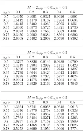
Table 4: Relative efficiency of cluster sampling over simple random sam-pling
M = 2, ρy = 0.01, µ = 0.5 ρb/ρ 0.1 0.2 0.3 0.4 0.5
0.5 1.4070 0.9001 0.9327 0.9626 0.9901 0.55 1.5112 1.4179 1.3137 1.1964 1.0634 0.6 1.6415 1.5402 1.4269 1.2995 1.1551 0.65 1.8090 1.6973 1.5725 1.4321 1.2730 0.7 2.0323 1.9069 1.7666 1.6089 1.4301 0.75 2.3450 2.2002 2.0384 1.8564 1.6502 0.78 2.6008 2.4402 2.2608 2.0590 1.8302
M = 4, ρy = 0.01, µ = 0.5 ρb/ρ 0.1 0.2 0.3 0.4 0.5
0.5 1.3797 0.8826 0.9146 0.9439 0.9709 0.55 1.4819 1.3904 1.2882 1.1731 1.0428 0.6 1.6096 1.5102 1.3992 1.2743 1.1327 0.65 1.7739 1.6644 1.5420 1.4043 1.2483 0.7 1.9928 1.8698 1.7323 1.5777 1.4024 0.75 2.2994 2.1575 1.9989 1.8204 1.6181 0.78 2.5503 2.3929 2.2169 2.0190 1.7946
M = 5, ρy = 0.01, µ = 0.5 ρb/ρ 0.1 0.2 0.3 0.4 0.5
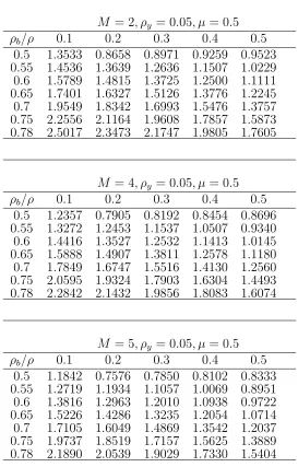
Table 5: Relative efficiency of cluster sampling over simple random sam-pling
M = 2, ρy = 0.05, µ = 0.5 ρb/ρ 0.1 0.2 0.3 0.4 0.5
0.5 1.3533 0.8658 0.8971 0.9259 0.9523 0.55 1.4536 1.3639 1.2636 1.1507 1.0229 0.6 1.5789 1.4815 1.3725 1.2500 1.1111 0.65 1.7401 1.6327 1.5126 1.3776 1.2245 0.7 1.9549 1.8342 1.6993 1.5476 1.3757 0.75 2.2556 2.1164 1.9608 1.7857 1.5873 0.78 2.5017 2.3473 2.1747 1.9805 1.7605
M = 4, ρy = 0.05, µ = 0.5 ρb/ρ 0.1 0.2 0.3 0.4 0.5
0.5 1.2357 0.7905 0.8192 0.8454 0.8696 0.55 1.3272 1.2453 1.1537 1.0507 0.9340 0.6 1.4416 1.3527 1.2532 1.1413 1.0145 0.65 1.5888 1.4907 1.3811 1.2578 1.1180 0.7 1.7849 1.6747 1.5516 1.4130 1.2560 0.75 2.0595 1.9324 1.7903 1.6304 1.4493 0.78 2.2842 2.1432 1.9856 1.8083 1.6074
M = 5, ρy = 0.05, µ = 0.5 ρb/ρ 0.1 0.2 0.3 0.4 0.5
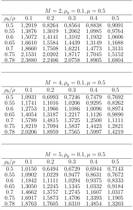
Table 6: Relative efficiency of cluster sampling over simple random sam-pling
M = 2, ρy = 0.1, µ = 0.5 ρb/ρ 0.1 0.2 0.3 0.4 0.5
0.5 1,2919 0,8264 0,8564 0,8838 0,9091 0.55 1,3876 1,3019 1,2062 1,0985 0,9764 0.6 1,5072 1,4141 1,3102 1,1932 1,0606 0.65 1,6610 1,5584 1,4439 1,3149 1,1688 0.7 1,8660 1,7508 1,6221 1,4773 1,3131 0.75 2,1531 2,0202 1,8717 1,7045 1,5152 0.78 2,3880 2,2406 2,0758 1,8905 1,6804
M = 4, ρy = 0.1, µ = 0.5 ρb/ρ 0.1 0.2 0.3 0.4 0.5
0.5 1,0931 0,6993 0,7246 0,7479 0,7692 0.55 1,1741 1,1016 1,0206 0,9295 0,8262 0.6 1,2753 1,1966 1,1086 1,0096 0,8974 0.65 1,4054 1,3187 1,2217 1,1126 0,9890 0.7 1,5789 1,4815 1,3725 1,2500 1,1111 0.75 1,8219 1,7094 1,5837 1,4423 1,2821 0.78 2,0206 1,8959 1,7565 1,5997 1,4219
M = 5, ρy = 0.1, µ = 0.5 ρb/ρ 0.1 0.2 0.3 0.4 0.5
0.5 1,0150 0,6494 0,6729 0,6944 0,7143 0.55 1,0902 1,0229 0,9477 0,8631 0,7672 0.6 1,1842 1,1111 1,0294 0,9375 0,8333 0.65 1,3050 1,2245 1,1345 1,0332 0,9184 0.7 1,4662 1,3757 1,2745 1,1607 1,0317 0.75 1,6917 1,5873 1,4706 1,3393 1,1905 0.78 1,8763 1,7605 1,6310 1,4854 1,3203
5. Conclusions
In sampling on two occasions we have considered the estimation of the sum of mean and the change of mean for current occasion when the sampling units are clusters and the observations on the first occasion are regarded as ancillary information for the observations on the second or current occasion. Under certain condition, the cluster sampling on two occasions is more efficient than the simple random sampling on two occasions.
increases with large increase in ρb (ρb > ρ) for the estimation of the change of mean. Further, for fixed ρb and ρ, the efficiency decreases with increase in ρy.
References
1. Artes Rodriguez, E. M. and Garcia Luengo, A. V. (2005). Multivariate indirect methods of estimation in successive sampling. J Ind. Soc. Agril. Statist, 59(2):97–103.
2. Das, A. (1982). Estimation of population ratio on two occasions. Journal of the Indian Society of Agricultural Statistics, 34(2):1–9.
3. Eckler, A. R. et al. (1955). Rotation sampling. The annals of mathematical statistics, 26(4):664–685.
4. Garcıa Luengo, A. V. and O˜na, I. (2010). The non-response in the change of mean and the sum of mean for current occasion in sampling on two occasions. Chilean Journal of Statistics, 2(1):63–84.
5. Gupta, P. (1979). Sampling on two successive occasions. Journal of Statis-tical Research, 13(13):7–16.
6. Hansen, M. H., Hurwitz, W. N., and Madow, W. G. (1953). Sample survey methods and theory. V. 1. Methods and applications. V. 2. Theory. Number 519.52 H249. Wiley.
7. Jessen, R. J. (1942). Statistical investigation of a sample survey for obtain-ing farm facts. Research Bulletin (Iowa Agriculture and Home Economics Experiment Station), 26(304):1.
8. Patterson, H. (1950). Sampling on successive occasions with partial replace-ment of units. Journal of the Royal Statistical Society. Series B (Method-ological), 12(2):241–255.
9. Pradhan, B. K. (2004). On efficiency of cluster sampling on sampling on two occasions. Statistica, 64(1):183–191.
10. Rao, J. and Graham, J. E. (1964). Rotation designs for sampling on repeated occasions. Journal of the American Statistical Association, 59(306):492–509.
11. Singh, G. and Singh, V. (2001). On the use of auxiliary information in successive sampling. Journal of the Indian Society of Agricultural Statistics, 54(1):1–12.
13. Sukhatme, P. and Sukhatme, B. (1970). Sampling theory of surveys with applications. Food and Agriculture Organization, Rome, Second edition.
14. Zarkovich, S. and Krane, J. (1965). Some efficient ways of cluster sampling.