Abstract—Natural stone tiles, which are used in decoration field, should be in a specific visual standard. In order to meet this expectation, it is very important that the tiles be classified before being packed. Especially in operation where exports of processed natural stones are increasing, all steps from cutting to packing must be done with the least mistakes. In the natural stone sector, selection workers are mostly used for classification and packaging operations. This situation; changing environmental factors such as light, temperature, can result in errors due to the fact that the human eye tends to get tired and lose perception over time. Therefore, there is a need for an automation system that can be used correctly for classification. Along with developing technologies, it is seen that the errors that can occur in classification can be reduced to a minimum. In this study both of supervised and unsupervised algorithms were used and it was tried to determine which classifier and dataset gave the most accurate result. Besides this, the corner fractures of the travertine tiles were also detected and quality control was made.
Index Terms—Travertine classification, surface analysis, bayes classification, quality control.
I. INTRODUCTION
Turkey is in the upper ranks between the world's major natural stone producers with its reserves and the developing natural stone industry. Export line of the sector is developing with the investments made. In particular, demand for processed natural stone from abroad is in a continuous increase [1].
Classification in the natural stone sector is mostly done by selection workers. In this manual classification process, mistakes are often encountered. The main reasons for this are; the workers used for classification are misclassified with environmental factors such as light and temperature and the occurrence of losses in perceptions of their employed for classification [2], [3].
Various studies are being made to solve this problem in the natural stone sector, which has an important place in the Turkish economy. Common view of these studies; it has been seen that an automation system working in place of the human hand at the classification stage will solve this problem to a great extent [2]-[6].
Classification methods, classify the data based on features
Manuscript received November 3, 2017; revised January 12, 2018. Nazan Kemaloglu is with the Department of Computer Engineering, Suleyman Demirel University, Turkey (e-mail: [email protected]).
Tuncay Aydogan is with the Department of Software Engineering, Suleyman Demirel University, Turkey (e-mail: [email protected]).
Sedat Metlek is with the Department of Mechatronics, Mehmet Akif Ersoy University, Turkey (e-mail: [email protected]).
that extracted from them. These features can be extracted from the given data with various operations [2], [4], [7], [8]. All extracted features may not be usable. At this point, selection process can be done with various feature selection algorithms [3], [8], [9].
In addition to classification, there is also the detection and quality control of fractures occurring in natural stones in the literature, morphological processing steps such as erosion, dilation, opening etc. are applied for this process [10]-[14].
In this study, travertine tiles are classified through the features that extracted and examined from them. In the course of classification, it has been tried to find a classification algorithm suitable to the dataset by using classification algorithms which are supervised and not unsupervised. Corner fractures were also detected, and broken natural stones were removed from dataset. All studies made with MATLAB R2015a.
II. MORPHOLOGICAL PRE-PROCESSING
A. Morphological Closing
Morphological closure is used to join the broken objects on the image and to fill in the gaps. The application is implemented on the binary image with the help of any structural element. The structural element to be used is circulated on the image and the closing operation is completed [15], [16]. The morphological closing process is expressed by Eq. (1).
(1) where, A is binary image as an input image and B is structural element.
III. FEATURE EXTRACTION
The values to be considered in the classification phase are the attributes that will represent the dataset in hand. With these features, the general characteristics of the classes can be established. On the other hand, classification makes use of different relations between these features to distinguish between the available data. Gray Level Co- Occurrence Matrices (GLCM) is one of the best known tissue analysis tools for calculating second order statistical features of the view [17].
The GLCM describes the relationship between neighboring pixels on the image. This relationship indicates the number of occurrences and the brightness levels in the pixel pairs at a constant distance and the direction [18]. Statistical properties such as contrast, energy, correlation and
Classification of Travertine Tiles with Supervised and
Unsupervised Classifiers and Quality Control
contrast can be calculated with GLCM.
A. Feature Extraction from Color Analysis
Texture represents the statistical properties of pixel density. Texture analysis is one of the methods used in feature extracting.
∑ (2)
∑ | | (3)
∑ -
(4)
∑ | |
(5) - ∑ (6)
where; is probability density function and are the mean and standard deviation of the rows and columns of [19].
B. Feature Extraction from Texture Analysis
Color spaces are mathematical models that represent colors. According to Grassmann's first law, each color is represented by 3 independent variables. For this reason, color spaces are modeled in 3D [20].
The RGB color space alone is not enough for the feature extraction phase. Therefore, other color spaces are also analyzed.
HLS color space, consist (H: Hue), (L: Lightness) and (S: Saturation) values. HLS is converted from RGB color space by non-linear methods as shown Eq. (7) [8] [21].
{ where ;
√ (7)
The LMS color space that obtained from RGB space by linear methods, consists of Long (L), Medium (M), Short (S) components as shown Eq. (8) [22].
[
] [ ] (8)
The OHTA color space that developed by Ohta in 1980, is a linear color space transformation. Ohta color space is obtained according to Eq. (9) [23] [24].
[
] [ ] (9) The YCbCr color space that obtained from RGB space by
linear methods, consists of Y (Luminance), Cb and Cr (chrominance information) components as shown Eq. (10) [25], [26].
[
] [ ] [ ] (10) YPbPr is a linearly transformed color space, representing the analog shape of the YCbCr color space [8] [27].
[
] [ ] (11)
- -
From color spaces, statistical data such as general average, standard deviation and gray thresh value can be obtained.
IV. FISHER FEATURE SELECTION ALGORITHM Fisher's feature selection algorithm, which uses arithmetic mean and standard deviation values of classes, is an effective method for filtering. With this method, it is possible to remove noisy data to obtain a subset of features in large data sets [28] [29]. Eq. 12 is used to find the transformation matrix to be used when selecting the existing features.
| | | | (12)
where; W is transformation matrix, is in-class scatter matrix and is inter-class scatter matrix.
Scatter matrices are given in Eq. 13 and Eq. 14.
∑ ∑ (13) ∑ (14) where; C is class number, is data number in each class, is m. data in each class, is average values of i. class and is total average for every data [3].
V. BAYESIAN CLASSIFICATION
Bayes, which is basically referred to as a hypothesis, approaches the classification process as a probabilistic problem [30] [31]. The properties used in Bayesian classifiers can be expressed as follows
{ } (15) where; is n sets of finite natural states (pattern recognition set) and
{ } (16) where; A is s possible decisions group and is defined as the d component feature vector.
( | ) ; is the conditional probability density function for ( ),
( ) ; is priori probability of natural ( ), | | | | ; is posteriori probability.
When the probabilities are combined with Bayes Rule;
( | |) ( | ) (17)
where; ( ) is,
( ) ∑ ( | ) (18)
By Bayes decision rule, if
( | |) ( | |) (19) Decision is; [31] [32] [33].
The Bayes decision rule shows how best the classifier should be designed, if known for preliminary probabilities and class conditional densities ( | ) [34].
VI. FUZZY C-MEANS CLASSIFICATION
The Fuzzy C-Means algorithms, which have the widest use of fuzzy clustering algorithms, aim to reduce the objective function [35], [36].
The Fuzzy C-Means algorithms allow each object to belong to more than one class. The algorithm assigns a membership value to each object in the range [0, 1] for each class. The sum of membership values for all classes is 1 and the class that has the greatest membership value is determined as the class to which the object belongs [8], [37]. In the algorithm, the optimum value is obtained by converging the objective function to the determined minimum value and classification is complete [38], [39].
The objective function is given in Eq. (20).
∑ ∑ ‖ ‖ (20)
where; is class’ pixel element, is cluster center, m is the center of gravity that controls the fuzzy by varying from 1 to ∞. After the initial membership matrix is randomly assigned, the center vectors are updated according to Eq. (21) and Eq. (22).
∑
∑ (21) U membership value is recalculated according to the
calculated cluster centers.
∑ (‖ ‖ ‖ ‖)
⁄
(22)
The membership matrix U containing the fuzzy values as a result of the operation shows the result of the clustering [8] [37].
VII. RESULTS
Travertine samples of two classes were used for the works. These class are called AT (Class-1) for first nine samples and KT (Class-2) for least nine samples, as shown in Fig. 1.
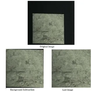
Fig. 1. Travertine tiles’ samples.
Firstly, background subtraction is applied all images. These images contain black background pixels. So the value read from the matrix is 10 pixels inside (Fig. 2).
Fig. 2. Getting the used image from original image.
For the fractal detection, image with background is used. Firstly, image converted to binary form. Then morphological closing is applied and image frame is detected. After this step the sum of pixel values (SPV) is calculated for quality control (QC). The total value differs according to the used resolution value. In this study, the sum of pixel values is determined to be 220000 and above, the sturdy tile (ST) and if less than 220000, the broken tile (BT) as shown Eq. (23) and Fig. 3.
{
{
Fig. 3. Fractal detection.
has been studied for classification. Total of 17 color spaces, including the RGB color space, were tested in this study. Various features were extracted by texture analysis from each color space (Table I).
TABLE I: EXTRACTED FEATURES
Feature Type Number of Features
Average of each color component 3 General average of color space 1 General standard deviation of color
space 1
Standard deviation of each color
component 3
Contrast 1
Homogeneity 1
Energy 1
Correlation 1
Entropy 1
Gray level threshold value 1
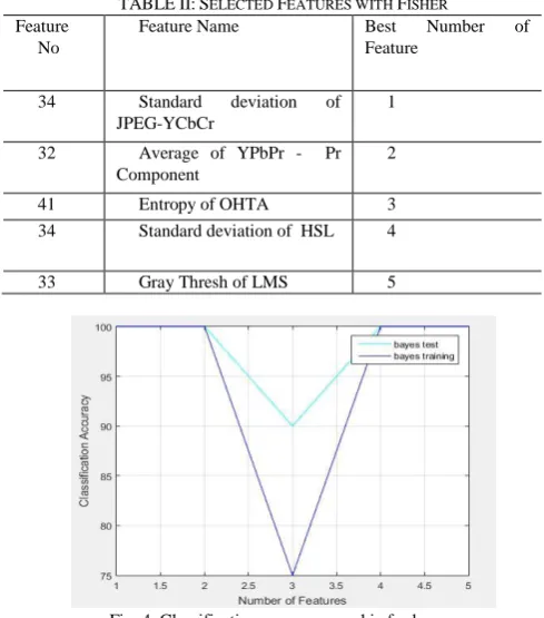
Features specified in Table I were extracted from 17 color spaces during the attribute extraction phase, and consequently, 238 features were obtained for each travertine. Not all of the features are suitable for use. Therefore, by examining the features, the ones that can distinguish 2 classes have been determined and reduced to 42 features. Five features were selected by Fisher feature selection algorithm in order to determine the most efficient for classification from the 42 features in the hand. Selected features are given in Table 2.
TABLE II: SELECTED FEATURES WITH FISHER Feature
No
Feature Name Best Number of Feature
34 Standard deviation of JPEG-YCbCr
1
32 Average of YPbPr - Pr Component
2
41 Entropy of OHTA 3
34 Standard deviation of HSL 4
33 Gray Thresh of LMS 5
Fig. 4. Classification accuracy graphic for bayes.
First, the selected 5 features are classified with Bayes, which is a supervised classification algorithm. The available feature matrix for Bayes is divided into 40% training and 60% test. Used for this step PR-Tools in MATLAB. This tool chooses training and test sets at different region in feature matrix for every time. The rate of recognition of the test data of the trained classifier by the training data is given in Fig. 2.
The numerical values of the same graph are shown in Table III.
TABLE III: CLASSIFICATION ACCURACY RATE FOR BAYES
Feature Name Classification
Accuracy Standard deviation of JPEG-YCbCr 100%
Average of YPbPr Pr 100%
Entropy of OHTA 90%
Standard deviation of HSL 100%
Gray Thresh of LMS 100%
General classification success 98%
The fuzzy C-means algorithm, which is one of the fuzzy clustering methods and is frequently used for classification in the literature, is used as an unsupervised classifier. Threshold values for 5 selected features were determined by Fisher feature selection algorithm and given to Fuzzy C-Means algorithms as input (Table IV).
TABLE IV: FUZZY C-MEANS’ THRESHOLD VALUES Thresh Feature Name AT
(Class-1) of Thresh
KT
(Class-2) of Thresh (T1) Standard
deviation of JPEG-YCbCr
(T1) <20 (T1) >20
(T2) Average of YPbPr Pr Component
(T2) <0.021
(T2) >0.02 1
(T3) Entropy of OHTA
(T3) <4.20 (T3) >4.20
(T4) Standard deviation of HSL
(T4) >90 (T4) <90
(T5) Gray Thresh of LMS
(T5) <0.55 (T5) >0.55
The membership values for Class- 1 (AT) and Class-2 (KT) of each data are given in Table V and Table VI.
TABLE V: MEMBERSHIP RATE FOR AT (CLASS– 1) Tile
No
Feature No
1 2 3 4 5
1 0.9956 0.9999 0.9957 0.8794 0.9129
2 0.9888 0.9864 0.9891 0.9993 0.9906
3 0.9677 0.9733 0.9677 0.8677 0.9652
4 0.9984 0.9970 0.9985 0.9448 0.9990
5 0.9872 0.9816 0.9872 0.9348 0.9962
6 0.9979 0.9999 0.9978 0.9122 0.9923
7 0.9439 0.9637 0.9439 0.9284 0.9564
8 0.9984 0.9977 0.9985 0.9531 0.9985
9 0.9773 0.9777 0.9776 0.9143 0.9520
10 0.9328 0.9518 0.9319 0.7553 0.8999
11 0.8370 0.9007 0.8351 0.6038 0.7399
12 0.7827 0.8334 0.7804 0.7912 0.8643
13 0.9152 0.9519 0.9119 0.9252 0.9681
14 0.1651 0.1900 0.1620 0.0234 0.2270
15 0.8976 0.8959 0.8957 0.6195 0.8945
16 0.0087 0.0075 0.0093 0.0107 0.0034
17 0.0577 0.0585 0.0588 0.0812 0.0547
18 0.0117 0.0224 0.0109 0.0002 0.0020
TABLE VI: MEMBERSHIP RATE FOR KT (CLASS– 2) Tile
No
Feature No
1 2 3 4 5
5 0.0128 0.0184 0.0128 0.0652 0.0038
6 0.0021 0.0001 0.0022 0.0878 0.0077 7 0.0561 0.0363 0.0561 0.0716 0.0436 8 0.0016 0.0023 0.0015 0.0469 0.0015 9 0.0227 0.0223 0.0224 0.0857 0.0480 10 0.0672 0.0482 0.0681 0.2447 0.1001 11 0.1630 0.0993 0.1649 0.3962 0.2601 12 0.2173 0.1666 0.2196 0.2088 0.1357 13 0.0848 0.0481 0.0881 0.0748 0.0319 14 0.8349 0.8100 0.8380 0.9766 0.7730 15 0.1024 0.1041 0.1043 0.3805 0.1055 16 0.9913 0.9925 0.9907 0.9893 0.9966 17 0.9423 0.9415 0.9412 0.9188 0.9453 18 0.9883 0.9776 0.9891 0.9998 0.9980
According to Table V and Table VI, the first 9 samples and samples 14, 16, 17, 18 were transferred to the right class, whereas the samples 10,11,12,13 and 15 were transferred to the wrong class. Looking at the same tables, it is seen that the sum of the membership rates of each sample in the same feature AT (Class-1) and KT (Class-2) is 1. The classification success is given in Table VII.
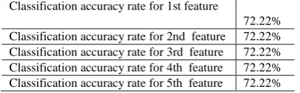
TABLE VII: CLASSIFICATION ACCURACY RATE FOR FUZZY C-MEANS Classification accuracy rate for 1st feature
72.22% Classification accuracy rate for 2nd feature 72.22% Classification accuracy rate for 3rd feature 72.22% Classification accuracy rate for 4th feature 72.22% Classification accuracy rate for 5th feature 72.22%
The classification performance given in Table VII was found to be the same for all features in fuzzy c-means algorithm.
VIII. CONCLUSION
A total of 18 samples of both classes were used in this study. The products’s size is 15 ×15 cm. In the detection of broken travertine, it was tried to find the exact area of the travertine. The threshold value determined for fracture detection can be changed according to the pixel values of the image So if this process is applied to products that are different sizes, the threshold value (SPV) will definitely change. Besides this, the process is worked only for corner fractures. It is predicted that a study can be made in the future, for detection small-scale fractures along the edges of the travertine.
The results obtained show that the data used is not suitable for unsupervized learning. The fuzzy C-Means algorithm failed to exceed 72.2% classification success, nevertheless, 98% success was achieved in classification with the supervised Bayes algorithm.
The result obtained compares Bayes and fuzzy c-means classifiers in the classification phase. The fuzzy C-Means algorithms have achieved a fairly low success rate against the Bayes classifier. This shows that the supervised classification algorithm is one of the most important elements that provides success in the data set. When classifying, comparison from pre-trained data is the most suitable method in the developed system.
The Fuzzy C-Means algorithms, which classify the data according to the degree of membership according to their
proximity to the determined cluster centers, failed to achieve the desired performance in the system. According to literature, the Fuzzy C-Means algorithms, which are frequently used clustering methods with a high success rate in the classification phase of the travertine tiles, are insufficient in this study. The reason for this is that the different in-class data are close together and the data is divided into two classes. It is envisaged that if number of samples are increased, classification accuracy can achieve a high success rate with Fuzzy C-Means algorithms.
ACKNOWLEDGMENT
The authors would like to thank to Süleyman Demirel University Research Project Coordination Unit (BAP) for support to 4536-YL1-16.
REFERENCES
[1] S. Yalçın and T. Uyanık, “The place of turkey in world marble trading,”
Turkey III. Marble Symposium 3-5 May 2001, s-397-416, Afyon. [2] M. A. Selver and O. Akay, “Evaluating clustering methods for
classification of marble slabs in an automated industrial marble inspection system,” in Proc. International Conference on Electrical and Electronics Engineering.
[3] S. Metlek, “Automatic classification of natural stone plate wıth machine vision,” Doctoral thesis, Suleyman Demirel Universty, Graduate School of Natural Sciences, Isparta, 2015.
[4] J. Martínez-Alajarín, J. D. Luis-Delgado, and L. M. Tomás-Balibrea, “Automatic system for quality-based classification of marble textures,”
IEEE Transactions on Systems, Man, and Cybernetics, Part C (Applications and Reviews), vol. 35, no. 4, 2005, pp. 488-497. [5] M. A. Selver, O. Akay, F. Alim, S. Bardakçı, and M. Ölmez, “An
automated industrial conveyor belt system using image processing and hierarchical clustering for classifying marble slabs,” Robotics and Computer-Integrated Manufacturing, vol. 27, no. 1, 2011, pp. 164-176.
[6] Ö. Akkoyun, “An evaluation of ımage processing methods applied to marble quality classification,”Turkey VII. International Marble and Natural Stone Congress, 2011.
[7] A. Selver, E. Ardali, and O. Akay, “Feature extraction for quantitative classification of marbles,” ISignal Processing and Communications Applications, pp. 1-4, 2007.
[8] M. Şişeci, “Determination of travertine plate stones with clustering methods,” Master thesis, Suleyman Demirel University, Graduate School of Natural Sciences, Isparta, 2012.
[9] A. Gümüşçü, İ. B. Aydilek, and R. Taşaltın, “Comparison of feature selection algorithms on microarray data classification,” Harran Universty Engineering Journal, vol. 1, no. 1, 2016.
[10] H. Elbehiery, A. Hefnawy, and M. Elewa, “Surface defects detection for ceramic tiles using ımage processing and morphological techniques,”World Academy of Science, Engineering and Technology International Journal of Computer, Electrical, Automation, Control and Information Engineering, vol. 1, no. 5, 2007, p. 52, 2005. [11] G. M. Rahaman and M. Hossain, “Automatic defect detection and
classification technique from image: A special case using ceramic tiles,”
International Journal of Computer Science and Information Security,
vol. 1, no. 1, May 2009.
[12] R. Gonydjaja and B. T. M. Kusuma, “Rectangulary defect detection for ceramic tile using morphological techniques,” ARPN Journal of Engineering and Applied Sciences, vol. 9, no. 11, 2014, pp. 2052-2056.
[13] G. Jacob, R. Shenbagavalli, and S. Karthika, “Detection of surface defects on ceramic tiles based on morphological techniques,” Cornell University Library, 2016.
[14] S. Singh and M. Kaur, “Machine vision system for automated visual inspection of tile’s surface quality,”IOSR Journal of Engineering, vol. 2, pp. 429-432, 2012.
[15] M. Karhan, M. O. Oktay, Z. Karhan, and H. Demir, “Detecting spots on apricots due to coryneum beijerinckii disease with morphological ımage processing methods,” in Proc. 6th International Advanced Technologies Symposium , pp. 172-176, 2011.
[16] R. C. Gonzales and R. E. Woods, “Digital ımage processing,” Second Edition, Prentice Hall, 2002.
mammogram and determination of the mass via artificial neural
network,”National Congress of Medical Technologies ’14, 2014. [18] Ö. Kayaaltı, B. H. Aksebzeci, İ. Ö. Karahan, K. Deniz, M. Öztürk, B.
Yılmaz, and M. H. Asyalı, “Liver fibrosis staging using CT image texture analysis and soft computing,”Applied Soft Computing, vol. 25, pp. 399-413, 2014.
[19] A. Demirhan and I. Guler, “Image segmentation using self-organizing maps and gray level co-occurrence matrices,”Journal of the Faculty of Engineering and Architecture of Gazi University, vol. 25, no. 2, pp. 285-291, 2010.
[20] İ. Yılmaz, M. Güllü, T. Baybura, and A. O. Erdoğan, “Color spaces and color conversion programme (CCP),” Afyon Kocatepe Universty Journal of Science and Engineering Sciences, vol. 2, no. 2, 2002, pp. 19-35.
[21] C. Balas, “An imaging colorimeter for noncontact tissue color mapping,”IEEE transactions on Biomedical Engineering, vol. 44, no. 6, 1997, pp. 468-474.
[22] E. Reinhard, M. Adhikhmin, B. Gooch, and P. Shirley, “Color transfer between images,”IEEE Computer Graphics and Applications, vol. 21, no. 5, pp. 34-41, 2001.
[23] V. Jayakrishna , G. P. Akhila, and S. Basher, “Advanced hybrid color space normalization for human face extraction and detection,”
International Journal for Scientific Research and Development,vol. 1, no. 4, 2013, pp-1043-1053.
[24] Y. I. Ohta, T. Kanade, and T. Sakai, “Color information for region segmentation,”Computer Graphics and İmage Processing, vol. 13, no. 3, pp. 222-241, 1980.
[25] X. Wang, C. Hu, and S. Yao, “An adult image recognizing algorithm based on naked body detection,” in Proc. ISECS International Colloquium on Computing, Communication, Control, and Management, 2009, pp. 197-200.
[26] J. A. M. Basilio, G. A. Torres, G. S. Pérez, L. K. T. Medina, and H. M. P. Meana, “Explicit image detection using YCbCr space color model as skin detection,” Applications of Mathematics and Computer Engineering, pp. 123-128, 2011.
[27] C. Scheffler and J. M. Odobez, “Joint adaptive colour modelling and skin, hair and clothing segmentation using coherent probabilistic index maps,”ın Proc. British Machine Vision Association-British Machine
Vision Conference, 2011.
[28] T. H. Dat and C. Guan, “Feature selection based on fisher ratio and mutual information analyses for robust brain computer interface,” in
Porc. IEEE International Conference on Acoustics, Speech and Signal Processing,pp. I-337, 2007.
[29] M. Kaya, Feature selection and Classification on Gene Expression Data, Master Thesis, Gazi Universty, Graduate School of Natural Sciences, Ankara, 2014
[30] R. O. Duda, P. E. Hart, and D. G. Stork, Pattern Classification Second Edition, 2000.
[31] A. Altınörs, E. Avcı, and Z. Biçer, “Using of the bayes decision rules classifier for digital modulation recognition system,” E- Journal of New World Sciences Academy, vol. 3, no. 1, 2008.
[32] E. Alpaydin, “Introduction to machine learning (adaptive computation and machine learning series,” The MIT Press Cambridge, 2004. [33] Y. Terzi, N. Murat, and M. A. Cengiz, “Bayesian hypothesis test and
bayes factor,”e- Journal of New World Sciences Academy, vol. 3, no. 2, pp-321-329, 2008.
[34] A. Karabulut, “Bayesian scene classification,” Master Thesis, Hacettepe Universty, Graduate School of Natural Sciences, Ankara, 2006.
[35] J. C. Dunn, “A fuzzy relative of the ISODATA process and its use in detecting compact well-separated clusters,”Well-Separated Clusters, J. Cybern., pp. 32-57, 1973.
[36] J. C. Bezdek, C. Coray, R. Gunderson, and J. Watson, (1981). Detection and characterization of cluster substructure i. linear structure: Fuzzy c-lines. SIAM Journal on Applied Mathematics,vol. 40, no. 2,
pp. 339-357, 1981.
[37] M. Işık and A. Y. Çamurcu, “Applied performance determination of k-means, k-medoids and fuzzy c-means algorithms,” Journal of İstanbul Ticaret Üniversitesi Graduate School of Natural Sciences, vol. 6, no. 11, pp. 31-45, 2007.
[38] S. Naz, H. Majeed, and H. Irshad, “Image segmentation using fuzzy clustering: A survey,” inPorc. 2010 6th International Conference on Emerging Technologies, 2010.
[39] E. Doğanay, S. Kara, and H. K. Özçelik, “Automatic segmentation of the lungs from HRCT scans by using fuzzy c- means clustering,” in
Porc. the Fifth International Symposium on Sustainable Development, 2014.
Nazan Kemaloğlu is a computer engineer and a postgraduate student at the Süleyman Demirel University
Tuncay Aydoğan received the PhD degree in 2005 from Sakarya University. He is currently an associated professor of Suleyman Demirel University. His research interests include smart systems, fuzzy logic, automatic control and ındustrial networks.