Testing for volatility co-movement in bivariate stochastic volatility models

ISSN: 2341-2356

Instituto

Complutense

de Análisis

Económico

Testing for Volatility Co-movement in

Bivariate Stochastic Volatility Models

Jinghui Chen

Graduate School of International Social Sciences Yokohama National University

Masahito Kobayashi

Department of Economics Yokohama National University

Michael McAleer

Department of Quantitative Finance National Tsing Hua University, Taiwan And Econometric Institute, Erasmus School of Economics Erasmus University Rotterdam

And Department of Quantitative Economics Complutense University of Madrid, Spain And Institute of Advanced Sciences Yokohama National University, Japan

Abstract

The paper considers the problem of volatility co-movement, namely as to whether two financial returns have perfectly correlated common volatility process, in the framework of multivariate stochastic volatility models and proposes a test which checks the volatility co-movement. The proposed test is a stochastic volatility version of the co-movement test proposed by Engle and Susmel (1993), who investigated whether international equity markets have volatility co-movement using the framework of the ARCH model.

In empirical analysis we found that volatility co-movement exists among closelylinked stock markets and that volatility co-movement of the exchange rate markets tends to be found when the overall volatility level is low, which is contrasting to the often-cited finding in the financial contagion literature that financial returns have co-movement in the level during the financial crisis.

Keywords Lagrange multiplier test; Volatility co-movement, Stock markets, Exchange rate Markets; Financial crisis

JEL Classification C12, C58, G01, G11 UNIVERSIDAD COMPLUTENSE MADRID

Working Paper nº 1710

February, 2017

Testing for Volatility Co-movement in

Bivariate Stochastic Volatility Models

Jinghui Chen

Graduate School of International Social Sciences

Yokohama National University

Masahito Kobayashi

Department of Economics

Yokohama National University

Michael McAleer

Department of Quantitative Finance

National Tsing Hua University, Taiwan

and

Econometric Institute, Erasmus School of Economics

Erasmus University Rotterdam

and

Department of Quantitative Economics

Complutense University of Madrid, Spain

and

Institute of Advanced Sciences

Yokohama National University, Japan

Revised: February 2017

∗_{corresponding author: Masahito Kobayashi, Department of Economics, Yokohama National University,}

Abstract

The paper considers the problem of volatility co-movement, namely as to whether two financial returns have perfectly correlated common volatility process, in the framework of multivariate stochastic volatility models and proposes a test which checks the volatility co-movement. The proposed test is a stochastic volatility ver-sion of the co-movement test proposed by Engle and Susmel (1993), who investi-gated whether international equity markets have volatility co-movement using the framework of the ARCH model.

In empirical analysis we found that volatility co-movement exists among closely-linked stock markets and that volatility co-movement of the exchange rate markets tends to be found when the overall volatility level is low, which is contrasting to the often-cited finding in the financial contagion literature that financial returns have co-movement in the level during the financial crisis.

Keywords: Lagrange multiplier test; Volatility co-movement, Stock markets, Exchange rate Markets; Financial crisis

1

Introduction

This paper considers the problem as to whether financial returns have volatility co-movement using the framework of multivariate stochastic volatility models that were suggested byHarvey et al. (1994). We propose a stochastic volatility version of the ARCH test proposed by Engle and Kozicki (1993) and Engle and Susmel (1993), who investigated volatility co-movement, namely whether international equity markets have a common volatility process, using the multi-variate ARCH model framework, and found groups of countries that had a similar time-varying volatility. Fleming et al. (1998) used the multivariate stochastic volatility model to estimate volatility linkages across stock, bond, and money markets, and found strong correlation between markets. Fleming et al. (1998) also tested perfectly correlated volatility processes, extending the model of Tauchen and Pitts. (1983). Their definition of volatility linkage is stronger than the mere presence of a common factor in volatility processes in that they have no idiosyncratic volatility factor. They also conducted a Wald-type test, using the GMM framework, and re-jected the null hypothesis of perfectly correlated volatility and concluded that cross-market hedging is imperfect.

However, the use of the Wald and likelihood ratio tests in the classical hypothesis testing framework, which use the estimator of the volatility correlation parameter, is inappropriate for the null hypothesis of perfectly correlated volatility, as the asymptotic distribution of the Wald test statistics is different from the conventional chi-squared distribution, as shown, for example, in Chernoff (1954), since, as the correlation estimator cannot be greater than or equal to one in absolute value, the distribution of the estimator of the constrained parameter is asymmetric, and hence non-normal, when the true correlation coefficient is unity under the null hypothesis. The paper proposes a new Lagrange multiplier (LM) test for volatility co-movement, namely the hypothesis that the volatility processes of bivariate series have a perfectly correlated com-mon volatility factor. We use the framework of multivariate stochastic volatility model proposed by Harvey et al. (1994), where the log volatility follows vector autoregressive (VAR) process of order one with diagonal autoregressive coefficient matrix.

The Lagrange multiplier test principle is the only alternative for this problem in deriving the test statistics because it estimates only the null model and does not estimate the parameter on the boundary of the parameter space. Then the test statistic can follow the conventional

chi-squared asymptotic distribution under the null hypothesis.

To the best of our knowledge, the Lagrange multiplier test statistic for the perfectly corre-lated volatility processes has not been proposed in the literature, except Chiba and Kobayashi

(2013), who employed the unconventional assumption that the log of squared returns is nor-mally distributed in deriving the test statistic. It is not without reason why the LM test has not been proposed; the conventional method to obtain a score function is unworkable in this problem, because the derivative of the transition density is intractable under the null hypoth-esis, as the transition disturbance has zero variance. We here derive the score function using the ingenious method devised byChesher (1984), which is the main technical breakthrough in tackling this problem.

Our test can be regarded as a test for the number of stochastic volatility factors, in line with the definition ofHarvey et al. (1994) and Cipollini and Kapetanios (2008), when the number of factors is one under the null hypothesis. Cipollini and Kapetanios (2008) used a linearized model for the log of squared returns, and used the principal component methodology ofStock and Watson (2002) in deciding the number of factors. Their method has the advantage in that it is applicable when the number of variables is large, though it is not a statistical test. The new test developed in the paper is the only existent statistical test for the hypothesis.

We employed the quadrature in evaluating the likelihood function proposed by Watanabe

(1999) and Kitagawa (1987) and the method proposed byHamilton (1989) in evaluating the score function.

The remainder of the paper is organized as follows. Section 2 presents the model, Section 3 develops the LM test statistic, Section 4 presents Monte Carlo experiments, and Section 5 illustrates two empirical analyses, and concluding remarks are given in Section 6. Appendices illustrate the pre-orthogonalization of data and the derivation of the score functions.

2

Model

We here consider the unconstrained bivariate stochastic volatility model. Under the alternative hypothesis, the observation vector yt= (y1t, y2t)0 is expressed as follows:

(Model under the Alternative Hypothesis):   y1t y2t  =   exph1t 2 0 0 exp(h2t 2 )     e1t e2t  , t= 1,· · · , T, (1)   h1t h2t  =   ρ 0 0 ψ     h1,t−1 h2,t−1  +   σ 0 ω √λ     u1t u2t  , t= 1,· · · , T, (2)   h11 h21  =   σ/p(1−ρ2_{) 0} ω/p(1−ψ2₎ p λ/(1−ψ2₎     u11 u21  , (3) (e1t, e2t, u1t, u2t) 0 ∼N(0,I4),

where the log volatility (h1t, h2t)0 follows a stationary bivariate autoregressive process of order

one, and disturbance term is normally distributed contemporaneously and serially independent with zero mean unit variance.

The null hypothesis to be tested is

(Null Hypothesis): λ = 0, ψ =ρ, ω=σ. (4)

Under the nullhypothesis the joint distribution of the state variable (h1t, h2t)0 is degenerate,

since the disturbance term of the transition equation (2) is (σu1t, ωu1t+

√

λu2t)0; then the

measurement equations have a single common volatility, which is expressed as

(Null Model):   y1t y2t   = exp(h1t/2)   e1t e2t  , (5) h1t = ρh1,t−1 +σe1t,, h2t =h1t, t= 1,· · · , T. (6)

The multivariate stochastic volatility model was originally suggested by Harvey et al. (1994) and was examined in detail in Danıelsson(1998) andAsai et al. (2006). The null model of our paper is the stochastic volatility factor model discussed in Harvey et al. (1994) and Cipollini and Kapetanios(2008) in the simple case when the number of factors is one.

A remark may be in order here on the assumption that the disturbance term of the mea-surement equation (1), namely (e1t, e2t)0, is contemporaneously uncorrelated. We can justify

the use of this simple assumption by showing in Appendices that the data can be transformed so as to satisfy the assumption of the model under the null hypothesis.

3

LM test statistic

3.1

Notation

We propose the LM test for the null hypothesis (4) for the observation seriesy1t andy2t. Define

the unconstrained parameter vector asθ1 = (c, ψ, ω, ρ, σ), and the constrained parameter vector

as θ0 = (0, ψ, ω, ψ, ω) .

First, we obtain the maximum likelihood estimator of the constrained parameter, θ0, of

the state space system (1) and (2). Denote y₁ = (y11, y12, . . . , y1T)

0 , y₂ = (y21, y22, . . . , y2T) 0 , h1 = (h11, h12, . . . , h1T) 0 , and h2 = (h21, h22, . . . , h2T) 0

. The likelihood is expressed as

f(y₁,y₂) =

Z Z

f(h1,h2,y1,y2)dh1dh2 =

Z Z

f(y₁,y₂|h1,h2)f(h2|h1)f(h1)dh1dh2,

where the explicit form of f(y₁|h1), f(y2|y1,h1,h2), f(h2|h1), and f(h1) are given in

Appen-dices. We perform this integration numerically by the quadrature suggested by Kitagawa

(1987) and Watanabe(1999) in evaluating the likelihood function.

Second, we derive the score function under the alternative hypothesis and evaluate it under the null hypothesis. Denote

y_T = (y11, y12, . . . , y1T, y21, y22, . . . , y2T)

0

= (y₁,y₂) and the score function as

∂logf(y_t) ∂θ1 = ∂logf(y_t) ∂λ , ∂logf(y_t) ∂ψ , ∂logf(y_t) ∂ω , ∂logf(y_t) ∂ρ , ∂logf(y_t) ∂σ .

Noting that logf(y_t|y_t−1) = logf(y_t)−logf(y_t−1), conditional score function is expressed as

Qt= ∂logf(y_t|y_t−1) ∂θ0₁ = ∂logf(y_t) ∂θ₁0 − ∂logf(y_t−1) ∂θ₁0 .

Then the estimated Fisher information matrix is

(Fisher Information Matrix): I(θ) = 1

T T X t=1 QtQ 0 t,

and the score vector is

(Score Vector): U(θ) = 1 T T X t=1 Qt = 1 T ∂logf(y_T) ∂θ₁0 . (7)

3.2

Test statistic

The LM test statistic is defined by

(LM Test Statistic): LM =T × U0(ˆθ0)I(ˆθ0)−1U(ˆθ0), (8)

where ˆθ0 is the maximum likelihood estimator of θ0 under the null hypothesis. Then, under the

regularity condition that the parameters to be estimated lie in the interior of the parameter space and the estimated information matrix converges to a nonsingular matrix, and hence the estimators are normally distributed asymptotically, we have

(Asymptotic Distribution): LM −→L χ2(3),

when T is sufficiently large, as shown by Davidson and MacKinnon (1993, p. 91), with three degrees of freedom of the asymptotic χ2-distribution corresponding to the three restrictions of the null hypothesis (4).

The score function (7) cannot be evaluated by the conventional method; the derivative

∂f(h2|h1)/∂λ in ∂f(y_t) ∂λ = Z f(y₁,y₂|h1,h2) ∂f(h2|h1) ∂λ f(h1)dh1dh2 (9)

diverges asλ→0, becausef(h2|h1) is a normal density with varianceλand hence its derivative,

as well as the score function, with respect λ under the null hypothesis cannot be evaluated directly. We have circumvented this difficulty using the ingenious method proposed inChesher

(1984). The algebraic details for the derivation of (10) are found Appendices. We here give only the final formula of the score functions as follows:

(Score Functions) ∂logf(y) ∂λ |H0 = 1 8trEh1|y −2×VψY2exp(−h1)11×T +1T×TVψ +VψY2exp(−h1) exp(−h 0 1)Y2−2VψY2H−11 , ∂logf(y) ∂ψ |H0 = 1 211×TV 1/2 ψ ZψEh1|y[h1]− 1 2tr h Y2V 1/2 ψ ZψEh1|y[h1exp(−h 0 1)] i , ∂logf(y) ∂ω |H0 =− 1 2ω11×TEh1|y[h1] + 1 2ω(y2◦y2) 0 Eh1|y[exp(−h1)◦h1], ∂logf(y) ∂ρ |H0 =− ∂logf(y) ∂ψ |H0 − ψ 1−ψ2 − 1 2ω −2 tr ∂V −1 ψ ∂ψ Eh1|y h1h 0 1 ! , ∂logf(y) ∂σ |H0 =− ∂logf(y) ∂ω |H0 − t ω + 1 ω3tr V−_ψ1Eh1|y h1h 0 1 , (10)

where◦denotes the operator of the element-by-element multiplication (the Hadamard product), exp(−h1) = (exp(−h11), . . . ,exp(−h1T))0, (11)

Y2 =diag(y2◦y2), (12)

H1 =diag(exp(h11), . . . ,exp(h1T)), (13)

and Vψ is the covariance matrix of h2, whose square root Vψ1/2 is defined by the Cholesky

decomposition.

The algebraic details of the derivation of (10) are found in Appendices.

4

Monte Carlo experiments

In order to confirm that the proposed statistic is asymptotically distributed as χ2_{(3) under}

the null, and whether it has power to reject a false hypothesis, we conduct two Monte Carlo experiments. The number of iterations is 1000 for the experiment under the null model and 100 for the experiment under the alternative hypothesis. The number of iterations of the latter is not large, but this limitation is unavoidable because the convergence of the maximum likelihood estimation is slow and hence the calculation of the test statistics require considerable computational time when the data is generated from the alternative hypothesis.

It took two minutes on the average to calculate one iteration for the data for Tables 1 and 2 when the sample size is 500 with the parallel computing tool of MATLAB (8 threads) using a PC with Intel’s Core I7 -3770K . The codes are available from the authors on request.

4.1

Size of Test and Null Distribution

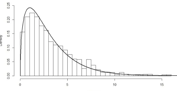
First, we generate artificial samples drawn from the null hypothesis, calculate the test statistic, and obtain the empirical distribution of the test statistic under the null hypothesis. Second, we estimate the empirical power by the ratio of the test statistic that exceeds the theoretical critical value. We also obtain the empirical distribution of the test statistic under the null and alternative hypotheses by using kernel estimation and histogram to show that it follows the

χ2(3) distribution with sufficient precision.

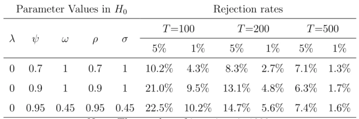
The rejection rates for some critical values and sample sizes are shown in Table 1, when the data is generated under the null hypothesis, where θ0 = (λ = 0, ψ, ω, ρ =ψ, σ=ω). Table

1 shows that, as the sample size T increases, the rejection rate approaches to the theoretical significance level. The empirical size of the test is sufficiently close to the theoretical value when the sample size is 500, which suggests that we should use data with at least 500 observations in practice. The empirical null distribution of the test statistic whenT = 500 is shown in Figures 1-3.

Table 1: Rejection Rates of the Null under the Null Hypothesis Parameter Values inH0 Rejection rates

λ ψ ω ρ σ T=100 T=200 T=500

5% 1% 5% 1% 5% 1%

0 0.7 1 0.7 1 10.2% 4.3% 8.3% 2.7% 7.1% 1.3% 0 0.9 1 0.9 1 21.0% 9.5% 13.1% 4.8% 6.3% 1.7% 0 0.95 0.45 0.95 0.45 22.5% 10.2% 14.7% 5.6% 7.4% 1.6%

Note: The number of iterations is 1000.

Figure 2: Histogram of LM Test Statistic at ψ=0.9

Figure 3: Histogram of LM Test Statistic atψ=0.95

4.2

Power of test

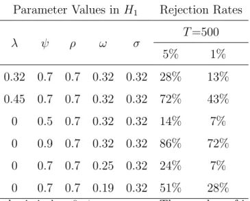
We generate artificial data under the alternative hypothesis, and calculate the rejection rate to show that the proposed statistic has sufficient power. The Monte Carlo results are shown in

Table 2, where the parameter value deviates from that of the null hypothesis. For example, the value of λ is set at 0.32 and 0.45 in the first and second rows under the alternative hypothesis, whereas it should be λ= 0 under the null hypothesis.

Table 2: Rejection Rates of the Null under the Alternative Hypothesis Parameter Values in H1 Rejection Rates

λ ψ ρ ω σ T=500 5% 1% 0.32 0.7 0.7 0.32 0.32 28% 13% 0.45 0.7 0.7 0.32 0.32 72% 43% 0 0.5 0.7 0.32 0.32 14% 7% 0 0.9 0.7 0.32 0.32 86% 72% 0 0.7 0.7 0.25 0.32 24% 7% 0 0.7 0.7 0.19 0.32 51% 28%

5

Empirical analysis

Using the proposed statistical test, we first examine the volatility co-movement between stock markets to find a group of countries with common volatility factor and show that our method can be applied to more than two markets. We next investigate the effect of overall volatility level on the co-movement of exchange rates by comparing the financial crisis period and low volatility period.

The value of the test statistic depends upon the the order of the variables in the pair and hence the empirical result is sometime inconsistent when the order is changed, because the pre-orthogonalization of data illustrated in Appendices is asymmetric with respect to the order of the variables. The null distribution of the test statistic is unaffected with respect to the order of variable when the the volatility co-movement exits under the null hypothesis by its construction; then, the the probability of type I error is correct after the pre-orthogonalization. Under the alternative hypothesis, however, the pre-orthogonalization can contaminate the joint distribution of the volatilities, and hence undermine the power of the test statistic.

We believe that we can solve this asymmetry problem in future by estimating the correlation parameter of the measurement equation in (1) simultaneously, by means of improvement in the accuracy and speed of the computation .

5.1

Stock markets

First, we checks whether there exists a group of stock markets that shows volatility co-movement consistently in different times. The data is the adjusted-close prices downloaded from Yahoo finance for the stock market indexes listed below:

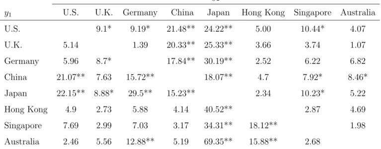
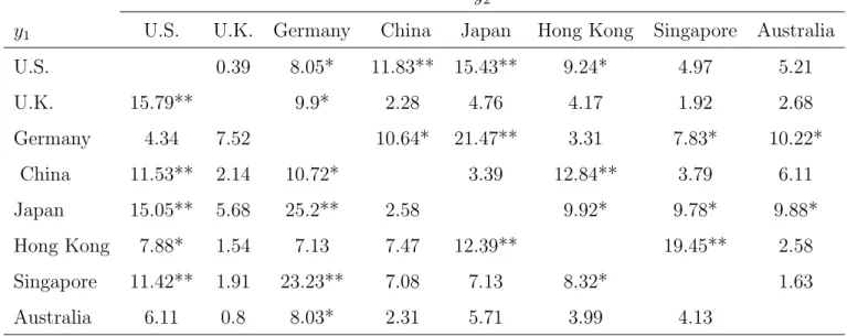
We divided daily data from January, 2011 to December, 2014 into two periods to check the volatility co-movement in different periods. We excluded observations whenever at least one market is closed. The test is performed for the 28 pairs, and we have 56 values in Tables 4 and 5, since the value of the test statistic depends upon the order of the variables asymmetrically, on account of the data pre-orthogonalization process in Appendices.

We see that U.K., Singapore, and Australia can share the same volatility factor consistently even in different periods, where the null hypothesis is accepted, even if calculated in the different order, for every possible pairs in the group. China and Japan have volatility factor independent

Table 3: Stock Market Indexes

Stock Market Symbol Country/Region

Dow Jones Industrial Average DOW U.S.

FTSE Index FTSE U.K.

DAX Index DAX Germany

Shanghai Composite Index SSCI China Nikkei 225 Stock Average Index NIKKEI Japan

Hang Seng Index HSI Hong Kong Straits Times Index STI Singapore All Ordinaries Index AORD Australia

Table 4: Test Statistic for Volatility Co-movement of Stock Markets for 2011-2012

y2

y1 U.S. U.K. Germany China Japan Hong Kong Singapore Australia

U.S. 9.1* 9.19* 21.48** 24.22** 5.00 10.44* 4.07 U.K. 5.14 1.39 20.33** 25.33** 3.66 3.74 1.07 Germany 5.96 8.7* 17.84** 30.19** 2.52 6.22 6.82 China 21.07** 7.63 15.72** 18.07** 4.7 7.92* 8.46* Japan 22.15** 8.88* 29.5** 15.23** 2.34 10.23* 5.22 Hong Kong 4.9 2.73 5.88 4.14 40.52** 2.87 4.69 Singapore 7.69 2.99 7.03 3.17 34.31** 18.12** 1.98 Australia 2.46 5.56 12.88** 5.19 69.35** 15.88** 2.68

Note: * denotes significance at five percent, ** denotes significance at one percent.

mutually and of the other countries or regions in 2011 and 2012, where the null hypothesis is rejected with, at least, one of the two test statistic values. In 2013 and 2014, the number of groups that possibly share the same volatility factor is increased to three, namely

Table 5: Test Statistic for Volatility Co-movement of Stock Markets for 2013-2014

y2

y1 U.S. U.K. Germany China Japan Hong Kong Singapore Australia

U.S. 0.39 8.05* 11.83** 15.43** 9.24* 4.97 5.21 U.K. 15.79** 9.9* 2.28 4.76 4.17 1.92 2.68 Germany 4.34 7.52 10.64* 21.47** 3.31 7.83* 10.22* China 11.53** 2.14 10.72* 3.39 12.84** 3.79 6.11 Japan 15.05** 5.68 25.2** 2.58 9.92* 9.78* 9.88* Hong Kong 7.88* 1.54 7.13 7.47 12.39** 19.45** 2.58 Singapore 11.42** 1.91 23.23** 7.08 7.13 8.32* 1.63 Australia 6.11 0.8 8.03* 2.31 5.71 3.99 4.13

Note: * denotes significance at five percent, ** denotes significance at one percent.

Group 1 : U.K., China, Japan

Group 2 : U.K., Hong Kong, Australia Group 3 : U.K., Singapore, Australia

Then U.K., Singapore and Australia share the same volatility factor consistently in the two period, probably because of their close economic ties.

We cannot suggest, at this stage, why the number of groups with possibly the same volatility factors increased. It is suspected that a determinant is the overall level of volatility and we will consider this hypothesis in the next subsection using the exchange rate data.

.

5.2

Exchange rate markets

We here investigate the volatility processes of the foreign exchange rates in the global financial crisis and the low volatility period.

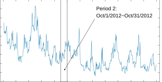
First, we define two time periods representing the financial crisis and the low volatility period using the Chicago Board Options Exchange (CBOE) Volatility Index (VIX) as an indicator of high volatility. Figures 4 and 5 show that volatility deviated drastically from the historical

trend in the financial crisis. We choose Period 1: Oct/1/2008 - Oct/31/2008 as the global financial crisis, and Period 2: Oct/1/2012 - Oct/31/2012 as low volatility period.

Figure 4: VIX during the Global Financial Crisis (2008-2009)

Jan/01/2008 Mar/01/2008 May/01/2008 Jul/01/2008 Sep/01/2008 Nov/01/2008 Jan/01/2009 Mar/01/2009 May/01/2009 Jul/01/2009 Sep/01/2009 Nov/01/2009 Jan/01/2010 10 20 30 40 50 60 70 80 90 Period 1: Oct/1/2008~Oct/31/2008

Figure 5: VIX during the Low Volatility Period (2012-2013)

Jan/01/2012 Mar/01/2012 May/01/2012 Jul/01/2012 Sep/01/2012 Nov/01/2012 Jan/01/2013 Mar/01/2013 May/01/2013 Jul/01/2013 Sep/01/2013 Nov/01/2013 Jan/01/2014 10 12 14 16 18 20 22 24 26 28 Period 2: Oct/1/2012~Oct/31/2012

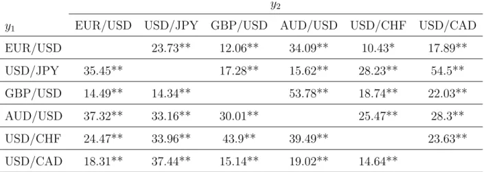
Second, we analyze 6 major currency pairs, namely Euro (EUR), the United States Dollar (USD), Japanese Yen (JPY), British Pound (GBP), Australian Dollar (AUD), Swiss Franc (CHF), Canadian Dollar (CAD), using roughly 500 hourly observations for a month, and the results of the proposed test of volatility co-movement are shown in Tables 6and 7.

Table 6: Test Statistic for Volatility Co-movement of Exchange Rates in High Volatility Period

y2

y1 EUR/USD USD/JPY GBP/USD AUD/USD USD/CHF USD/CAD

EUR/USD 23.73** 12.06** 34.09** 10.43* 17.89** USD/JPY 35.45** 17.28** 15.62** 28.23** 54.5** GBP/USD 14.49** 14.34** 53.78** 18.74** 22.03** AUD/USD 37.32** 33.16** 30.01** 25.47** 28.3** USD/CHF 24.47** 33.96** 43.9** 39.49** 23.63** USD/CAD 18.31** 37.44** 15.14** 19.02** 14.64**

Note: * denotes significance at five percent, ** denotes significance at one percent. The ex-change rate was downloaded from FXDD’s historical database.

Table 7: Test Statistic for Volatility Co-movement of Exchange Rates in Low Volatility Period

y2

y1 EUR/USD USD/JPY GBP/USD AUD/USD USD/CHF USD/CAD

EUR/USD 11.27* 5.17 7.56 6.61 25.69** USD/JPY 15.88** 28.67** 12.97** 16.73** 14.86** GBP/USD 2.15 23.74** 20.35** 5.39 8.38* AUD/USD 28.07** 18.32** 26.51** 14.97** 22.86** USD/CHF 3.22 9.53* 4.64 6.9 17.66** USD/CAD 5.5 6.47 4.83 5.82 4.41

Note: * denote significance at five percent, ** denotes significance at one percent. The exchange rates data was downloaded from FXDD’s historical database.

During the financial crisis, when volatility is large, the null hypothesis of volatility co-movement was rejected in every case in Table 6. On the other hand, several currency pairs are suggested to share the same volatility factor during the low volatility period; the accepted rate of the null hypothesis is 43.3%, namely 13 pairs of 30 pairs, in Table 7. Then we can suggest that the volatility co-movement tends to be found during the low volatility period. This result is interesting and contrasting to the often-cited finding in the financial contagion literature that financial returns have co-movement in the level during the financial crisis, which is discussed critically byForbes and Rigobon (2002) . It is suspected that, when the overall volatility level is low, the idiosyncratic volatility factor can be small, or often negligible, in comparison with the common volatility factor, whereas, when the overall volatility level is high in the financial crisis, the idiosyncratic volatility factor dominates the common volatility factor.

6

Conclusion

In this paper, we have proposed a Lagrange multiplier test statistic for the null hypothesis that the volatility processes of a bivariate series are perfectly correlated in the framework of the multivariate stochastic volatility model. The considered model is the simplest case of a multiple stochastic volatility model. The extension to a multiple factor model is left for further research, as it is a challenging problem computationally and theoretically. In order to improve the efficiency of the numerical calculation we are planning to use the particle filter method proposed by Kitagawa (1996) and the fast Gauss transform method proposed by Greengard and Strain (1991).

In the empirical analysis of stock markets, we found that the United Kingdom, Singapore and Australia share a common time-varying volatility factor consistently. It is also suspected that the common volatility factor in the global currency market was dominated by the idiosyn-cratic volatility factors during high volatility periods. A clear-cut conclusion cannot be obtained because of the asymmetry of the test statistic with respect to the order of the variables, which is left to the further research.

Appendices

A

Derivation of likelihood and score functions

A.1

Likelihood

In order to express the transition equation (2) in matrix form, we express the log volatilities and disturbance terms used in (1) and (2) in vector form, as follows:

h1 = (h11, . . . , h1t)0, h2 = (h21, . . . , h2t)0,

u1 = (u11, . . . , u1T)0, u2 = (u21, . . . , u2T)0,

e1 = (e11, . . . , e1T)0, e2 = (e21, . . . , e2T)0.

Then the transition equation (2) is

h1 =V1/2ρ (σu1), h2 =V 1/2 ψ (ωu1+ √ λu2) = V 1/2 ψ (V −1/2 ρ h1ω/σ+ √ λu2), (14)

where Vρ and Vψ are the covariance matrices of the autoregressive processes of order one, h1

andh2, respectively, and V1/2ρ andV 1/2

ψ are defined by their Cholesky decomposition as follows:

Vρ= (V1/2ρ )(V 1/2 ρ ) 0 , Vψ = (V 1/2 ψ )(V 1/2 ψ ) 0 , where V1/2_ψ =            1/p1−ψ2 _{0 . . . 0 0} ψ/p1−ψ2 _{1 . . . 0 0} ψ2_/p 1−ψ2 _{ψ . . . 0 0} .. . ψT−1_/p 1−ψ2 _ψT−2 _{. . . ψ 1}            , V1/2_ρ =            1/p1−ρ2 _{0 . . . 0 0} ρ/p1−ρ2 _{1 . . . 0 0} ρ2_/p 1−ρ2 _{ρ . . . 0 0} .. . ρT−1_/p 1−ρ2 _ρT−2 _{. . . ρ 1}            , (15)

Their inverses are decomposed as Vψ−1 = (V −1 2 ψ ) 0_V−12 ψ , Vρ −1 = (V− 1 2 ρ )0V −1 2 ρ , where: V− 1 2 ψ =               p 1−ψ2 _{0 . . . 0 0} −ψ 1 . . . 0 0 0 −ψ . . . 0 0 0 0 . . . 0 0 .. . 0 0 . . . −ψ 1               , V− 1 2 ρ =               p 1−ρ2 _{0 . . . 0 0} −ρ 1 . . . 0 0 0 −ρ . . . 0 0 0 0 . . . 0 0 .. . 0 0 . . . −ρ 1               . (16)

Then the density functions of the transition and measurement equations of the model is

f(h1) = 1 (2π)T2σT V −1/2 ρ exp −1 2σ −2 h0₁V−_ρ1h1 , (17) f(h2|h1) = 1 (2π)T2( √ λ)T V −1/2 ψ exp −1 2u 0 2u2 , (18) f(y₁|h1) = 1 (2π)T2 H −1/2 1 exp −1 2y 0 1H −1 1 y1 , (19) f(y₂|h2) = 1 (2π)T2 H −1/2 2 exp −1 2y 0 2H −1 2 y2 , (20) where u2 = V− 1 2 ψ h2−V −1 2 ρ h1 ω σ / √ λ, (21)

H1 =diag(exp(h11), . . . ,exp(h1T)),H2 =diag(exp(h21), . . . ,exp(h2T)). (22)

Then, we can rewrite the likelihood function as

(Likelihood): f(y₁,y₂) = Z Z f(y₂|h2)f(y1|h1)f(h2|h1)f(h1)dh2dh1, (23) where f(u2|h1) = 1 (2π)T2 exp −1 2u 0 2u2 (24) in terms ofu2, instead of h2, by the variable transformation (21).

A.2

Score function with respect to

λ

We obtain the score function with respect toλ as

∂f(y)

∂λ =

Z Z _∂f(y

2|u2,h1)

because the variance parameter λ appears only in f(y₂|h1,u2) = 1 (2π)T2 H −1/2 2 exp −1 2y 0 2H −1 2 y2

through h2 inH2 =diag(exp(h2)), since we have

h2 =V −1 2 ψ √ λu2+V −1 2 ρ ω σh1 (26) from (14).

Then we obtain the derivative of f(y₂|h1,u2,) with respect to λ as follows. First, noting

(26), we define f(y₂|h1,u2) =KF, (27) where K=|H2| −1/2 = exp −1 211×Th2 = exp −1 211×TV 1/2 ψ √ λu2+V −1 2 ψ ω σh1 , F= exp −1 2y 0 2H −1 2 y2 = exp −1 2(exp(−h2)) 0 (y₂◦y₂) (28)

and, for notational convenience, we define

exp(−h2) = (exp(−h21), . . . ,exp(−h2T))0,y2◦y2 = y212 , y222 , . . . , y2T2 0

and h2 denotes a function of u2 as the abbreviation of equation (26).

Then, defining M1 = ∂K ∂λ 1 √ λ, M2 = ∂F ∂λ 1 √ λ, (29) we have B= lim λ→0 ∂f(y) ∂λ = lim λ→0 Z (other terms) F∂K ∂λ +K ∂F ∂λ du2dh1 = lim λ→0 √ λR (other terms)(F M1+K M2)du2dh1 λ (30)

from (25). We then have that ∂K ∂λ =− 1 2K 1 2√λ11×TV 1/2 ψ u2 =− 1 4√λK 11×TV 1/2 ψ u2, ∂F ∂λ =− 1 2F ∂ ∂λexp(−h 0 2)(y2◦y2) = 1 4√λF G, G=u0₂V1/2_ψ 0 H−₂1(y₂◦y₂), (31) since ∂h2 ∂λ = 1 2√λV 1/2 ψ u2, ∂exp(−h2) ∂λ =− 1 2√λH −1 2 V 1/2 ψ u2.

Note that the denominators of the derivatives (31) and (29) contain λ, which converges to zero, and hence is intractable by conventional method. We will use the ingenious method proposed by Chesher (1984) to solve this singularity. First, applying L’Hopital’s rule with respect to λ , we obtain

B = 1₂B+ lim

λ→0

√

λ_∂λ∂ R(other terms)(F M1+K M2)du2dh1. (32)

Comparing the both sides of equation (32), we have

B= 2 lim λ→0 √ λ Z (other terms) ∂F ∂λ M1+ ∂K ∂λ M2 +F ∂M1 ∂λ +K ∂M2 ∂λ du2dh1 = 2 lim λ→0 √ λ Z (other terms) 2M1 M2+F ∂M1 ∂λ +K ∂M2 ∂λ du2dh1. (33)

Defining Y2 =diag(y2◦y2), the terms in the integrand are

M1M2 = − 1 4K 11×TV 1/2 ψ u2× 1 4F u 0 2V 1/2 ψ 0 Y2exp(−h2), ∂M1 ∂λ = − 1 4 ∂K ∂λ11×TV 1/2 ψ u2 = 1 16√λK tr(1T×TV 1/2 ψ u2u 0 2V 1/2 ψ 0 ), ∂M2 ∂λ = 1 4 ∂F ∂λG+ 1 4F ∂G ∂λ = 1 16√λFG 2 + 1 4F ∂G ∂λ , ∂G ∂λ = u 0 2V 1/2 ψ 0 Y2 ∂exp(−h2) ∂λ =− 1 2√λtr V1/2_ψ 0 Y2H−21V 1/2 ψ u2u 0 2 , G2 = u0₂V1/2_ψ 0 Y2exp(−h2) exp(−h 0 2)Y2V 1/2 ψ u2 = tr V1/2_ψ 0 Y2exp(−h2) exp(−h 0 2)Y2V 1/2 ψ u2u 0 2 .

Then, we have B= 1 8λlim→0 Z f(y₁|h1) 1 (2π)T2 KF −2tr 11×TV 1/2 ψ u2u 0 2V 1/2 ψ 0 Y2exp(−h2) +tr 1T×TV 1/2 ψ u2u 0 2V 1/2 ψ 0 +tr V1/2_ψ 0 Y2exp(−h2) exp(−h 0 2)Y2V 1/2 ψ u2u 0 2 − 2tr V1/2_ψ 0 Y2H−21V 1/2 ψ u2u 0 2 f(u2|h1)f(h1)du2dh1. (34)

We can perform the integration with respect to u2 in (34) analytically. As u2|h1 follows the

T-dimensitonal standard normal distribution, we have that

Z

u2u

0

2f(u2|h1)du2 =IT. (35)

Under the null hypothesis h2 =h1 and ψ =ρ, equation (34) is

B = 1 8 Z f(y₁|h1) 1 (2π)T2 KFh−2tr11×TV1/2ρ V 1/2 ρ 0 Y2exp(−h1) + tr1T×TV1/2ρ V 1/2 ρ 0 + trV1/2_ρ 0 Y2exp(−h1) exp(−h 0 1)Y2V1/2ρ − 2trV1/2_ρ 0 Y2H−11V 1/2 ρ i f(h1)dh1. (36) Noting that Vρ = V1/2ρ V 1/2 ρ 0

and applying the cyclic property of the trace operator to simplify the equation (36), we have

B= ∂f(y) ∂λ H0 = Z trJf(y,h1)dh1, (37) where J= 1 8 −2 (11×TVρY2exp(−h1)) +1T×TVρ +VρY2exp(−h1) exp(−h 0 1)Y2−2VρY2H−11 . (38) Since we have ∂logf(y) ∂λ H0 = lim λ→0 1 f(y) ∂f(y) ∂λ = Z trJ 1 f(y)f(h1,y)dh1 =trEh1|y(J) (39)

fromf(h1|y) =f(h1,y)/f(y),we have only to evaluateEh1|y[exp(−h1)] andEh1|y

exp(−h1) exp(−h1)

0

to obtain the score function. These expected values have no analytic expressions so that they should be evaluated numerically.

A.3

Score function with respect to

ψ

In the log-likelihood function, ψ appears only in f(y₁|h1,u2) = KF in (27). The partial

derivative of the likelihood with respect to ψ is

∂f(y) ∂ψ = Z ∂K ∂ψK −1 + ∂F ∂ψF −1 f(y,u2,h1)du2dh1 = Z ∂K ∂ψK −1 + ∂F ∂ψF −1 f(y,h1)dh1, (40)

since, as will be seen later, u2 can be integrated out in ∂K ∂ψK −1 +∂_∂ψFF−1 . Then we have ∂logf(y) ∂ψ H0 = Z ∂K ∂ψK −1 + ∂F ∂ψF −1 f(h1|y)dh1 =Eh1|y ∂K ∂ψK −1 +∂F ∂ψF −1 , (41) noting that f(h1|y) = f(h1,y)/f(y).

First, using (28) and the formula

∂V1/2_ψ ∂ψ =−V 1/2 ψ ZψV 1/2 ψ , (42) where Zψ = ∂V−_ψ1/2 ∂ψ , we have that ∂K ∂ψ =− 1 2K11×T ∂V1/2_ψ ∂ψ √ λu2+V −1 2 ρ ω σh1 = 1 2K11×TV 1/2 ψ ZψV 1/2 ψ √ λu2+V −1 2 ρ ω σh1 , ∂F ∂ψ =− 1 2F ∂ ∂ψ [(y2◦y2) 0 exp(−h2)] =−1 2F (y2◦y2) 0 H−₂1V1/2_ψ ZψV 1/2 ψ √ λu2+V −1 2 ρ ω σh1 , (43) as we have h2 =V 1/2 ψ √ λu2+V −1 2 ρ ω σh1 , (44) and hence ∂ ∂ψh2 = ∂V1/2_ψ ∂ψ √ λu2+V −1 2 ρ ω σh1 . (45)

Evaluating these terms under the null hypothesis λ= 0 and σ=ω, we have ∂K ∂ψ|H0 = 1 2K11×TV 1/2 ψ Zψh1, (46) ∂F ∂ψ|H0 =− 1 2F tr h Y2V 1/2 ψ Zψh1exp(−h 0 1) i , (47) using the identity

(y₂◦y₂)0H₁−1 = exp(−h0₁)Y2.

Then, from (41), we have

∂logf(y) ∂ψ H0 = 1 211×TV 1/2 ρ ZρEh1|y[h1]− 1 2tr h Y2V1/2ρ ZρEh1|y[h1exp(−h 0 1)] i . (48) Note that the matrix Y2V1/2ρ Zρ is lower triangular, and we have only to calculate the upper

triangular part of the matrix Eh1|y[h1exp(−h

0

1)] in evaluating the score function (48).

A.4

Score function with respect to

ω

First, note that, in the log-likelihood function, ω appears only in f(y₂|h1,u2) = KF, through

h2 =V 1/2 ψ √ λu2+V −1 2 ρ ω σh1 , (49)

as shown in (27). Then, we have the formula

∂logf(y) ∂ω =Eu2,h1|y ∂K ∂ωK −1₊ ∂F ∂ωF −1 , (50) using ∂f(y) ∂ω = Z (y₁|h1) ∂f(y₂|h1,u2) ∂ω f(h1)f(u2|h1)du2h1 = Z ∂K ∂ωK −1₊∂F ∂ωF −1 f(y,h1)dh1, (51) as we have ∂f(y₂|h1,u2) ∂ω = ∂K ∂ωF+K ∂F ∂ω = ∂K ∂ωK −1 + ∂F ∂ωF −1 f(y₂|h1,u2). (52)

From (28) their partial derivatives ofK and F are

∂K ∂ω H0 =−1 2K11×T 1 σh1, ∂F ∂ω H0 =−1 2F ∂ ∂ω[(y2◦y2) 0 exp(−h2)] H0 = 1 2F tr (y₂◦y₂)0H2 1 σh1 H0 , (53)

noting that, under the null hypothesis, we have ρ=ψ,h1 =h2, and Vρ=Vψ and ∂ ∂ω exp(−h2) =−H −1 2 ω/σ. Then we have ∂logf(y) ∂ω |H0 = − 1 2σ11×TEh1|y[h1] + 1 2σtr (y₂◦y₂)0Eh1|y[exp(−h1)◦h1] . (54)

A.5

Score function with respect to

ρ

In the log-likelihood function,ρappears only in f(y1|h1,u2) = KFand f(h1) in (17) and (27).

Then we have the derivative using the formula

∂logf(y) ∂ρ H0 =Eh1|y ∂K ∂ρK −1 +∂F ∂ρF −1 +∂f(h1) ∂ρ f(h1) −1 (55) analogously to that of (41). Noting (28) and (17) and defining

Zρ =

∂V−_ρ1/2

∂ρ , (56)

the derivatives of Kand F are

∂K ∂ρ = − 1 2K11×TV 1/2 ψ Zρ ω σh1, (57) ∂F ∂ρ = 1 2F (y2 ◦y2) 0 H−₁1V1/2_ψ Zρ ω σh1, (58) ∂f( h1) ∂ρ = f(h1) " − ρ 1−ρ2 − 1 2σ −2_tr ∂V −1 ρ ∂ρ h1h 0 1 !# . (59) We have used (∂/∂ρ) V 1/2 ρ = 1/ p

1−ρ2 _{in deriving the first term of equation (59). Noting}

that exp(−h10)Y2 = (y2 ◦y2)0H

−1

1 under the null hypothesis, we have

∂K ∂ρ|H0 =− 1 2K h 11×TV1/2ρ Zρ ω σh1 i =−∂K ∂ψ|H0, (60) ∂F ∂ρ|H0 =− 1 2F tr h Y2V1/2ρ Zρ ω σh1exp(−h 0 1) i =−∂F ∂ψ|H0. (61)

The score function with respect to ρ is

∂logf(y) ∂ρ |H0 =− ∂logf(y) ∂ψ |H0 − ρ 1−ρ2 − 1 2σ −2_tr ∂V −1 ρ ∂ρ Eh1|y h1h 0 1 ! . (62)

A.6

Score Function with respect to

σ

In the likelihood, σ appears only in K,F in (28) and f(h1). Then we can derive the score

function with respect to σ using the formula analogous to that of ρ given in (55), with ρ

replaced by σ. We can easily show from (28) that, under the null hypothesis ω = σ, the derivatives of K and F with respect to σ are equal to the negative of the derivations with respect to ω , namely ∂K ∂σ|H0 = − ∂K ∂ω|H0, (63) ∂F ∂σ|H0 = − ∂F ∂ω|H0, (64)

so that no additional calculations are necessary. From (17), the derivative of f(h1) is

∂f(h1) ∂σ =f(h1) −t σ + 1 σ3tr V−_ρ1h1h 0 1 . (65)

Using the formula

∂logf(y) ∂σ H0 =Eh1|y ∂K ∂σK −1₊∂F ∂σF −1₊∂f(h1) ∂σ f(h1) −1 , (66) whose derivation is analogous to that of (55), and comparing the formua (50), we have

∂logf(y) ∂σ |H0 =− ∂logf(y) ∂ω |H0 − t σ + 1 σ3tr V−_ρ1Eh1|y h1h 0 1 . (67)

B

Pre-orthogonalization of data

B.1

Purpose

Before estimating the model using actual data the observed return variables should be or-thogonalized so that the error terms (e1t, e2t) in the measurement equation (5) are distributed

contemporaneously independently with unit variance according to the assumption in (5), since the actual financial returns are contemporaneously correlated.

We cannot estimate the model under the assumption that (e1t, e2t)0 have non-zero

correla-tion and non-unit variances, because the increased number of the parameters to be estimated increases the computational time of the maximum likelihood estimation considerably. This problem is especially serious when the volatility series has high autocorrelation. We believe that this difficulty can be removed in future by improved algorithm. At present, however, this

assumption is unavoidable to perform Monte Carlo experiments reported in Section 4 with sufficient number of iterations

We here show that, if the null hypothesis is true, namely h1t ≡ h2t, we can orthogonalize

the observed series so as to satisfy the assumption of uncorrelatedness in (5).

This pre-orthogonalization is not without cost. The most serious demerit is that the result of the test depends upon the order of variables; we have a different value of the test statistic by exchanging the order of the variables, because the second variable is redefined by the Cholesky decomposition.

This asymmetry could be removed by including the correlation parameter in the measure-ment equation in (5) explicitly and then by estimating it simultaneously by the maximum likelihood method. However, we cannot use this method because the computational time is prohibitively large if the correlation parameter is included, so that we are obliged to drop the correlation parameter from (5) and to orthogonalize data before executing the test in the empirical analysis in Section 6.

B.2

Algebraic details

We assume that under the null hypothesis h1t = h2t for any t and that the actual data, say

(˜y1t, y˜2t), is written as (Unorthogonalized Model):   ˜ y1t ˜ y2t  = exp h_1t 2 A   e1t e2t  , A=   α1 0 α3 α2  , (68)

in practice, namely when the disturbance term of the measurement equation has non-zero correlation and non-unit variance, instead of (5). This assumption is justifiable because the proposed Lagrange multiplier test statistic uses only the estimation of the null model.

We here estimate A−1, which is the desired orthogonalization matrix. First, note that the product moment of (˜y1t,y˜2t) is Λ ≡E   ˜ y2 1t y˜1ty˜2t ˜ y1ty˜2t y˜22t  = E(exp(h1t))AA0. (69)

We can estimate Λ consistently using the sample moment of (˜y2

1t, y˜1ty˜2t, y˜2t2). Then we have

only to estimate E(exp(h1t)) in order to obtain A using the formula

where Λ1/2 _{denotes the Cholesky decomposition of Λ defined in (69).} Defining   ¨ y1t ¨ y2t  ≡Λ −1/2   ˜ y1t ˜ y2t  , (71) we have that   ¨ y1t ¨ y2t  =A −1_(E(exp(h 1t)))−1/2   ˜ y1t ˜ y2t  = (E(exp(h1t)))−1/2exp(h1t/2)   e1t e2t  , and hence

log ¨y2_1t=−log(E(exp(h1t))) +h1t+ loge21t.

Then, since we have E(log(e2

1t)) = −1.27 as shown by Harvey et al. (1994) and E(h1t) = 0

from the stationarity ofh1t, we have that

1

T

X

log ¨y_1t2 ≈E[log ¨y2_1t] =−log(E(exp(h1t)))−1.27

and hence we can estimate E(exp(h1t)) in (70) by

E(exp(h1t))≈exp

−(1/T)Xlog ¨y_1t2 + 1.27

.

Then we can have the orthogonalized data in (5) by

  y1t y2t  = ˆA −1   ˜ y1t ˜ y2t  , where ˆ A−1 = exph−(1/T)Xlog ¨y_1t2 + 1.27/2iΛˆ−12, (72) ˆ Λ = 1 T   P ˜ y2 1t P ˜ y1ty˜2t P ˜ y1ty˜2t Py˜2t2  . (73)

Acknowledgement

The authors are grateful to anonymous reviewers for very helpful comments and suggestions. This research is partially supported by the Grants-in-aid for Scientific Research of Japan Society for the Promotion of Science (C) 15K03394. The third author acknowledges the Australian Re-search Council and the National Science Council, Ministry of Science and Technology (MOST), Taiwan.

References

Asai, M., McAleer, M. and Yu, J. (2006). Multivariate stochastic volatility: A review.

Econo-metric Reviews, 25(2-3):145–175.

Chernoff, H. (1954). On the distribution of the likelihood ratio. The Annals of Mathematical

Statistics, 25(3):573–578.

Chesher, A. (1984). Testing for neglected heterogeneity. Econometrica, 52(4):865–872.

Chiba, M. and Kobayashi, M. (2013). Testing for a single-factor stochastic volatility in bivariate series. Journal of Risk of Financial Management, 6(1):31–618.

Cipollini, A. and Kapetanios, G. (2008). A stochastic variance factor model for large datasets and an application to S&P data. Economics Letters, 100(1):130–134.

Danıelsson, J. (1998). Multivariate stochastic volatility models: estimation and a comparison with vgarch models. Journal of Empirical Finance, 5(2):155–173.

Davidson, R. and MacKinnon, J. G. (1993). Estimation and inference in econometrics. Oxford University Press.

Engle, R. F. and Kozicki, S. (1993). Testing for common features. Journal of Business &

Economic Statistics, 11(4):369–380.

Engle, R. F. and Susmel, R. (1993). Common volatility in international equity markets. Journal

of Business & Economic Statistics, 11(2):167–176.

Fleming, J., Kirby, C. and Ostdiek, B. (1998). Information and volatility linkages in the stock, bond, and money markets. Journal of Financial Economics, 49(1):111–137.

Forbes, K. J. and Rigobon, R. (2002). No contagion, only interdependence: measuring stock market comovements. The Journal of Finance, 57(5):2223–2261.

Greengard, L. and Strain, J. (1991). The fast Gauss transform. SIAM Journal on Scientific

and Statistical Computing, 12(1):79-94.

Hamlton, J. D. (1989). A new approach to the economic analysis of nonstationary time series and the business cycle. Econometrica, 57(2):357–384.

Harvey, A., Ruiz, E. and Shephard, N. (1994). Multivariate stochastic variance models. The

Review of Economic Studies, 61(2):247–264.

Kitagawa, G. (1987). Non-Gaussian state-space modeling of nonstationary time series [with discussion] Journal of the American Statistical Association, 82(1):1032–1063.

Kitagawa, G. (1995). Monte Carlo filter and smoother for non-Gaussian nonlinear state space models Journal of Computational and Graphical Statistics, 5(1):1–125.

Stock, J. H. and Watson, M. W. (2002). Forecasting using principal components from a large number of predictors. Journal of the American Statistical Association, 97(460):1167–1179. Tauchen, G. E. and Pitts, M. (1983). The price variability-volume relationship on speculative

markets. Econometrica, 51(2):485–505.

Watanabe, T. (1999). A non-linear filtering approach to stochastic volatility models with an application to daily stock returns. Journal of Applied Econometrics, 14(2):101–121.