Ray: A Distributed Execution Engine for the Machine Learning Ecosystem

(1)

UC Berkeley

UC Berkeley Electronic Theses and Dissertations

Title

Ray: A Distributed Execution Engine for the Machine Learning Ecosystem Permalink https://escholarship.org/uc/item/3r5069pj Author Moritz, Philipp C Publication Date 2019 Peer reviewed|Thesis/dissertation

eScholarship.org Powered by the California Digital Library University of California

(2)

by

Philipp C Moritz

A dissertation submitted in partial satisfaction of the

requirements for the degree of

Doctor of Philosophy in Computer Science in the Graduate Division of the

University of California, Berkeley

Committee in charge:

Professor Michael I. Jordan, Chair Professor Ion Stoica

Professor Ken Goldberg

(3)

Ray: A Distributed Execution Engine for the Machine Learning Ecosystem

(4)

Abstract

Ray: A Distributed Execution Engine for the Machine Learning Ecosystem by

Philipp C Moritz

Doctor of Philosophy in Computer Science University of California, Berkeley Professor Michael I. Jordan, Chair

In recent years, growing data volumes and more sophisticated computational procedures have greatly increased the demand for computational power. Machine learning and artificial intelligence applications, for example, are notorious for their computational requirements. At the same time, Moores law is ending and processor speeds are stalling. As a result, distributed computing has become ubiquitous. While the cloud makes distributed hardware infrastructure widely accessible and therefore offers the potential of horizontal scale, devel-oping these distributed algorithms and applications remains surprisingly hard. This is due to the inherent complexity of concurrent algorithms, the engineering challenges that arise when communicating between many machines, the requirements like fault tolerance and straggler mitigation that arise at large scale and the lack of a general-purpose distributed execution engine that can support a wide variety of applications.

In this thesis, we study the requirements for a general-purpose distributed computa-tion model and present a solucomputa-tion that is easy to use yet expressive and resilient to faults. At its core our model takes familiar concepts from serial programming, namely functions and classes, and generalizes them to the distributed world, therefore unifying stateless and stateful distributed computation. This model not only supports many machine learning workloads like training or serving, but is also a good fit for cross-cutting machine learning applications like reinforcement learning and data processing applications like streaming or graph processing. We implement this computational model as an open-source system called Ray, which matches or exceeds the performance of specialized systems in many application domains, while also offering horizontally scalability and strong fault tolerance properties.

(5)

i

To my parents Hugo and Birgit, and my sistersChristine and Sophie,

(6)

6 Use Case: Large Scale Optimization 61 6.1 Introduction . . . 61 6.2 The Algorithm . . . 63 6.3 Preliminaries . . . 64 6.4 Convergence Analysis . . . 66 6.5 Related Work . . . 68 6.6 Experimental Results . . . 69 6.7 Proofs of Preliminaries . . . 71 6.8 Discussion . . . 74 7 Conclusion 76 Bibliography 79

(8)

List of Figures

2.1 Building an inverted index with MapReduce . . . 6

2.2 Neural network task graph, source https://www.tensorflow.org/guide/graphs . . 7

2.3 A chatroom implementation in the actor framework . . . 9

3.1 This figure depicts the SparkNet architecture. . . 13 3.2 Computational models for different parallelization schemes. . . 22 3.3 This figure shows the speedup τ Ma(b, τ, K)/Na(b) given by SparkNet’s

paral-lelization scheme relative to training on a single machine to obtain an accuracy of a = 20%. Each grid square corresponds to a different choice of K and τ. We show the speedup in the zero communication overhead setting. This experiment uses a modified version of AlexNet on a subset of ImageNet (100 classes each with approximately 1000 images). Note that these numbers are dataset specific. Nevertheless, the trends they capture are of interest. . . 23 3.4 This figure shows the speedups obtained by the naive parallelization scheme and

by SparkNet as a function of the cluster’s communication overhead (normalized so that C(b) = 1). We consider K = 5. The data for this plot applies to training a modified version of AlexNet on a subset of ImageNet (approximately 1000 images for each of the first 100 classes). The speedup obtained by the naive parallelization scheme is C(b)/(C(b)/K +S). The speedup obtained by SparkNet is N_a(b)C(b)/[(τ C(b) +S)M_a(b, K, τ)] for a specific value of τ. The numerator is the time required by serial SGD to achieve an accuracy of a, and the denominator is the time required by SparkNet to achieve the same accuracy (see Equation 3.1 and Equation 3.2). For the optimal value of τ, the speedup is maxτNa(b)C(b)/[(τ C(b) +S)Ma(b, K, τ)]. To plot the SparkNet speedup curve,

we maximize over the set of values τ ∈ {1,2,5,10,25,100,500,1000,2500} and use the values M_a(b, K, τ) and N_a(b) from the experiments in the fifth row of Figure 3.3. In our experiments, we have S ≈20s and C(b)≈2s. . . 24 3.5 This figure shows the performance of SparkNet on a 3-node, 5-node, and 10-node

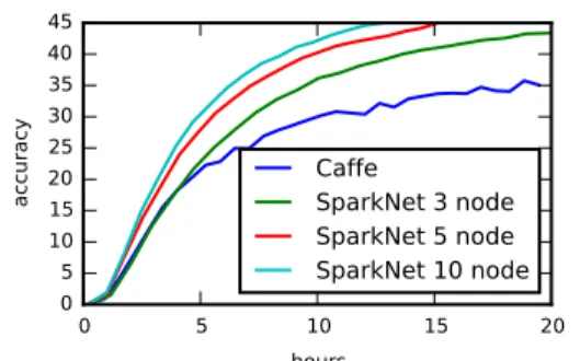
cluster, where each node has 1 GPU. In these experiments, we use τ = 50. The baseline was obtained by running Caffe on a single GPU with no communication. The experiments are performed on ImageNet using AlexNet. . . 25

(9)

v

3.6 This figure shows the performance of SparkNet on a 3-node cluster and on a 6-node cluster, where each 6-node has 4 GPUs. In these experiments, we use τ = 50. The baseline uses Caffe on a single node with 4 GPUs and no communication overhead. The experiments are performed on ImageNet using GoogLeNet. . . . 25 3.7 This figure shows the dependence of the parallelization scheme described in

Sec-tion 3.2 on τ. Each experiment was run with K = 5 workers. This figure shows that good performance can be achieved without collecting and broadcasting the model after every SGD update. . . 25

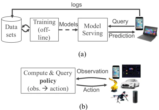
4.1 (a) Traditional ML pipeline (off-line training). (b) Example reinforcement learning

pipeline: the system continously interacts with an environment to learn a policy, i.e.,

a mapping between observations and actions. . . 27

5.1 Example of an RL system. . . 36

5.2 Typical RL pseudocode for learning a policy. . . 36

5.3 Python code implementing the example in Figure 5.2 in Ray. Note that @ray.remote

in-dicates remote functions and actors. Invocations of remote functions and actor methods return futures, which can be passed to subsequent remote functions or actor methods to encode task dependencies. Each actor has an environment object self.env shared

between all of its methods. . . 40

5.4 The task graph corresponding to an invocation of train policy.remote() in Figure 5.3.

Remote function calls and the actor method calls correspond to tasks in the task graph. The figure shows two actors. The method invocations for each actor (the tasks labeled

A1i and A2i) have stateful edges between them indicating that they share the mutable

actor state. There are control edges from train policy to the tasks that it invokes. To

train multiple policies in parallel, we could call train policy.remote() multiple times. 41

5.5 Ray’s architecture consists of two parts: an application layer and a systemlayer. The

application layer implements the API and the computation model described in Sec-tion 5.2, the system layer implements task scheduling and data management to satisfy

the performance and fault-tolerance requirements. . . 42

5.6 Bottom-up distributed scheduler. Tasks are submitted bottom-up, from drivers and

workers to a local scheduler and forwarded to the global scheduler only if needed

(Sec-tion 5.3). The thickness of each arrow is propor(Sec-tional to its request rate. . . 44

5.7 An end-to-end example that adds a and b and returns c. Solid lines are data plane

operations and dotted lines are control plane operations. (a) The function add() is

registered with the GCS by node 1 (N1), invoked onN1, and executed onN2. (b)N1

gets add()’s result using ray.get(). The Object Table entry forc is created in step 4

(10)

5.8 (a) Tasks leverage locality-aware placement. 1000 tasks with a random object depen-dency are scheduled onto one of two nodes. With locality-aware policy, task latency remains independent of the size of task inputs instead of growing by 1-2 orders of magni-tude. (b) Near-linear scalability leveraging the GCS and bottom-up distributed sched-uler. Ray reaches 1 million tasks per second throughput with 60 nodes. x∈ {70,80,90}

omitted due to cost. . . 48

5.9 Object store write throughput and IOPS. From a single client, throughput exceeds

15GB/s (red) for large objects and 18K IOPS (cyan) for small objects on a 16 core instance (m4.4xlarge). It uses 8 threads to copy objects larger than 0.5MB and 1 thread for small objects. Bar plots report throughput with 1, 2, 4, 8, 16 threads.

Results are averaged over 5 runs. . . 49

5.10 Ray GCS fault tolerance and flushing. . . 50

5.11 Ray fault-tolerance. (a)Ray reconstructs lost task dependencies as nodes are removed

(dotted line), and recovers to original throughput when nodes are added back. Each

task is 100ms and depends on an object generated by a previously submitted task. (b)

Actors are reconstructed from their last checkpoint. At t = 200s, we kill 2 of the 10

nodes, causing 400 of the 2000 actors in the cluster to be recovered on the remaining

nodes (t= 200–270s). . . 51

5.12 (a) Mean execution time of allreduce on 16 m4.16xl nodes. Each worker runs on a

distinct node. Ray* restricts Ray to 1 thread for sending and 1 thread for receiving.

(b) Ray’s low-latency scheduling is critical for allreduce. . . 52

5.13 Images per second reached when distributing the training of a ResNet-101 TensorFlow

model (from the official TF benchmark). All experiments were run on p3.16xl instances connected by 25Gbps Ethernet, and workers allocated 4 GPUs per node as done in Horovod [116]. We note some measurement deviations from previously reported, likely due to hardware differences and recent TensorFlow performance improvements. We

used OpenMPI 3.0, TF 1.8, and NCCL2 for all runs. . . 53

5.14 Time to reach a score of 6000 in the Humanoid-v1 task [21]. (a)The Ray ES

implemen-tation scales well to 8192 cores and achieves a median time of 3.7 minutes, over twice as fast as the best published result. The special-purpose system failed to run beyond 1024 cores. ES is faster than PPO on this benchmark, but shows greater runtime variance.

(b)The Ray PPO implementation outperforms a specialized MPI implementation [97]

with fewer GPUs, at a fraction of the cost. The MPI implementation required 1 GPU for every 8 CPUs, whereas the Ray version required at most 8 GPUs (and never more

than 1 GPU per 8 CPUs). . . 55

6.1 The left figure plots the log of the optimization error as a function of the num-ber of passes through the data for SLBFGS, SVRG, SQN, and SGD for a ridge regression problem (Millionsong). The middle figure does the same for a support vector machine (RCV1). The right plot shows the training loss as a function of the number of passes through the data for the same algorithms for a matrix completion problem (Netflix). . . 68

(11)

vii

6.2 These figures show the log of the optimization error for SLBFGS, SVRG, SQN, and SGD on a ridge regression problem (millionsong) for a wide range of step sizes. 69 6.3 These figures show the log of the optimization error for SLBFGS, SVRG, SQN,

(12)

List of Tables

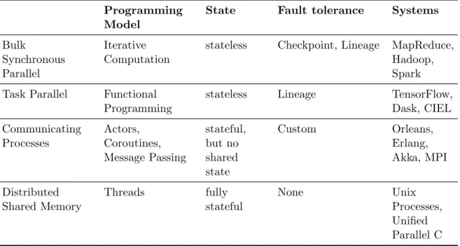
2.1 The spectrum of distributed computing . . . 4 5.1 Ray API . . . 38

5.2 Tasks vs. actors tradeoffs. . . 38

5.3 Throughput comparisons for Clipper [30], a dedicated serving system, and Ray for two

embedded serving workloads. We use a residual network and a small fully connected network, taking 10ms and 5ms to evaluate, respectively. The server is queried by clients

that each send states of size 4KB and 100KB respectively in batches of 64. . . 54

5.4 Timesteps per second for the Pendulum-v0 simulator in OpenAI Gym [21]. Ray allows

(13)

ix

Acknowledgments

I am deeply grateful to the many people who were part of my PhD journey. They helped me to grow professionally and as a person, and have made my time at Berkeley unforgettable. Without them this thesis would not have been possible. I would like to thank:

My advisor Michael Jordan for bringing me to Berkeley, for inspiring and encouraging me throughout my PhD, for bringing together such an exceptional and supportive group of peers and for motivating all of us with his kindness, enthusiasm and positivity.

My advisor Ion Stoica for mentoring me. His obsession with real-world impact and research that truly matters is unparalleled. He taught me many valuable lessons about research, systems design, planning, products and execution and truly expanded my horizon. Robert Nishihara, who has influenced my PhD journey like nobody else. His ability to confidently bust through any obstacle that might arise has greatly inspired me and helped me to not only see, but also reach the light at the end of the tunnel.

John Schulman with whom I collaborated closely at the beginning of my PhD. We have had many great conversations over the years and he has been a source of inspiration and ideas ever since!

Cathy Wu for countless discussions about research and life, her kindness and all the unforgettable memories we forged.

I would like to thank all the members of the Ray team, including Stephanie Wang, Eric Liang, Richard Liaw, Devin Petersohn, Alexey Tumanov, Peter Schafhalter, Si-Yuan Zhuang, Zongheng Yang, William Paul, Melih Elibol, Simon Mo, William Ma, Alana Marzoev, and Romil Bhardwaj. Thanks for a great collaboration. I have learned a lot from you!

I would like to thank my friends and colleagues from the research groups I have been part of. SAIL has been incredible. It is hard to describe the amount of knowledge and ideas that were transferred at our weekly research meetings, and the positivity and support from all of you, including Stefanie Jegelka, Ashia Wilson, Horia Mania, Mitchell Stern, Tamara Broderick, Ahmed El Alaoui, Esther Rolf, Chi Jin, Max Rabinovich, Nilesh Tripuraneni, Karl Krauth, Ryan Giordano, John Duchi, and Nick Boyd. The AMPLab, RISELab and BAIR have been a great community of friends and collaborators. Berkeley is unique for its collaborative research style, and the lab culture plays a major role in that.

I would like to thank my quals and thesis committee, Ken Goldberg, Joey Gonzalez and Fernando Perez for their insights, advice and support over the years!

My friend Fanny Yang for constant friendship and support, the many races and memories. You truly made a difference!

Many friends who made this journey unforgettable, including Fan Wei, Olivia Anguli, Richard Shin, Frank Li, Atsuya Kumano, Jordan Sullivan, Vinay Ramasesh, Jacob Stein-hardt, Ludwig Schmidt, Reinhard Heckel, Jacob Andreas, Alyssa Morrow, Jeff Mahler, Mehrdad Niknami, Smitha Milli, Marc Khoury and Sasha Targ.

My home for the last five years, a big house on the south side of Berkeley, called “Little Mountain”. Rishi Gupta for founding it and everybody living there for the great time we had together.

(14)

I would like to thank the Nishihara family for so kindly inviting and integrating me into many family gatherings and making me feel at home in the Bay area.

This thesis is dedicated to my family. My parents Hugo and Birgit, who created the right environment for me to thrive. Their unconditional love and support have made all the difference. My sisters Christine and Sophie for being awesome life companions, for their support and guidance over the year.

(15)

1

Chapter 1

Introduction

We are living in a remarkable time. In the span of a single human lifetime, we have seen the birth of machines that can process data, automatically perform tasks and make decisions. They have grown to have substantial real-world impact. If you are looking for any piece of information, there is a good chance that Google can find it for you. If you want to buy a product or get recommendations on what to buy, there is a large number of services on the internet that will help you to spend money, including Amazon. If you want to quickly get from A to B without having to worry about the details, ride sharing services like Uber or Lyft are the way to go. And not only our personal lives but also society crucially depends on our digital infrastructure. Science, education, our health care system and public administration as well as corporations would be unable to operate and coordinate the work of so many people without the help of computers. Computers are capable of running such diverse workloads as crunching numbers for scientific simulations, running complex queries on relational data to help operate large corporations or connecting people around the globe, and they are slowly starting to perform some of the complex cognitive tasks that only humans were capable of in the past. And fast forward another human lifetime, we will look back and realize that todays capabilities pale in comparison to what will be possible then.

Much of the computation is happening in the cloud, a large collection of servers that can be rented from providers like Amazon, Microsoft or Google. We typically use “edge” devices like smartphones or laptops to interface with the digital world, but in most cases the actual logic is implemented in the cloud. You become painfully aware of this if your phone gets disconnected from the internet and many important applications stop working. There are good reasons to shift much of the processing into the cloud: Moore’s law is ending, therefore single-core performance is not getting much faster, which means compute heavy application logic needs a large number of cores, which are typically only available on a cluster. Computing in the cloud also improves resource usage as processors can be shared between users and applications. One of the most important reasons why companies typically prefer running application logic in the cloud rather than the edge is control: They can determine the compute environment, have full access to the data and can secure private data and algorithms more easily.

(16)

Given this trend, it is quite surprising that distributed programming in the cloud is still very hard. Distributed systems is one of the more complex topics in computer science and while there is a large amount of research in this field, there is less work on making it easier for non-experts to build distributed software. If they want flexible systems, programmers typically have to build distributed applications from low-level primitives like remote pro-cedure call layers, distributed key-value stores and cluster managers, which requires a lot of expertise, duplicates work between different distributed systems and makes the task of debugging a distributed application even harder than it already is. Clearly distributed pro-gramming in the cloud is not yet as easy as propro-gramming on a laptop where programmers can choose from a rich set of high-level libraries, write complex applications with ease by composing them, and inspect the flow of the program and stop and debug it if something goes wrong.

These observations especially apply in the fields of machine learning and artificial intelli-gence. In fact, artificial intelligence is one of the most computationally expensive workloads due to ever increasing sizes of models and datasets. Many distributed systems have been developed to handle the scale of these applications: There are distributed data processing systems like MapReduce, Hadoop or Spark, stream processing systems like Flink or Kafka, distributed training systems like distributed TensorFlow, PyTorch or MxNet, distributed model serving systems like TensorFlow Serving or Clipper, and hyperparameter search tools like Vizier. However, each of these systems have a fairly narrow design scope. Therefore, in order to build end-to-end applications, practitioners often have to glue several systems together, which incurs high costs: Data needs to be converted at the system boundaries with costs for both development productivity and runtime efficiency, different fault toler-ance mechanisms need to be combined into an overall strategy, each of the systems needs to be managed and resources need to be allocated for each of them, which can lead to poor cluster utilization. Even worse, emerging workloads such as reinforcement learning, online learning and other cross-cutting applications need more flexible programming models and have stringent performance requirements that often cannot be fulfilled by gluing together existing systems. Practitioners are therefore often left to write their own distributed systems for such workloads from low-level primitives, reinventing many mechanisms of distributed systems like scheduling, data transfer or failure handling.

In this thesis, we instead advocate for a different approach. Instead of gluing together separate distributed systems, different workloads like data processing, streaming, distributed training and model serving should instead be implemented as reusable distributed libraries that run on top of one general-purpose system. The system should expose a programming model that is close to the programming models developers are familiar with from the single machine setting. This allows to expose common functionality like debugging, monitoring, dis-tributed scheduling and fault tolerance through an underlying disdis-tributed system and allows us to bring the cluster programming experience much closer to programming a laptop. The main contribution of this thesis is in designing a programming model for distributed com-putation and an implementation of that model which can support a wide variety of different distributed computing workloads, including the machine learning and artificial intelligence

(17)

CHAPTER 1. INTRODUCTION 3

applications mentioned above. The system and a number of libraries for different applica-tions have been implemented together with a large number of collaborators at Berkeley and many collaborators from both the wider open source community and various companies.

The thesis is organized as follows:

• In chapter 2, we give an overview over the spectrum of existing distributed program-ming models from more specialized to general. This gives the reader an appreciation of the design space and motivates the design decisions we make for the Ray programming model.

• In chapter 3, we describe a system for distributed training that we built on top of Apache Spark, which uses the BSP model, one of the programming models described in chapter 2. The shortcomings of this approach, together with the insights from our work in reinforcement learning (see [114] and [112]) were the main motivations for the design of Ray. This material was previously published in [83].

• In chapter 4, we study the requirements of a general purpose distributed system that can support emerging artificial intelligence applications like reinforcement learning. This material was previously published in [93].

• In chapter 5, the main chapter of the thesis, we describe the design and implementation of Ray. By decoupling the control and data plane and introducing stateful actors, it can fulfill the requirements outlined in chapter 4 and serves as an execution engine for a diverse set of tasks in distributed machine learning. This material was previously published in [82].

• In chapter 6, we present an algorithm for large-scale optimization with a linear con-vergence rate that is well-suited for the Ray architecture described in chapter 5. This material was previously published in [81].

(18)

Chapter 2

The Distributed Computation

Landscape

To get more context on how a flexible distributed system should be designed, let us first review existing solutions to make sure we are not reinventing the wheel and understand the design space. In this chapter, we will focus on practical systems for distributed computing (as opposed to research systems that demonstrate the viability of specific ideas). We will also view these systems under the lens of theirprogramming model, because that’s their most important characteristic for users and for building distributed applications.

In table 2.1 we give an overview over existing parallel and distributed programming

Programming Model

State Fault tolerance Systems

Bulk

Synchronous Parallel

Iterative Computation

stateless Checkpoint, Lineage MapReduce,

Hadoop, Spark

Task Parallel Functional

Programming

stateless Lineage TensorFlow,

Dask, CIEL Communicating Processes Actors, Coroutines, Message Passing stateful, but no shared state Custom Orleans, Erlang, Akka, MPI Distributed Shared Memory Threads fully stateful None Unix Processes, Unified Parallel C

(19)

CHAPTER 2. THE DISTRIBUTED COMPUTATION LANDSCAPE 5

models. The simplest way to do parallel computing is by executing a given function on a number of data items in parallel and storing the results. This is the SIMD (single instruction, multiple data) model, which is of course not sufficient, since more often than not the results need to be aggregated. SIMD plus aggregation is the Bulk Synchronous Parallel (BSP) model that we consider in section 2.1. Generalizing this pattern to arbitrary functions and data dependencies, but still keeping pure functions and not supporting stateful computation, gives the task parallel model, see section 2.2. Many applications like reinforcement learning or interactive serving systems need state however, which motivates extending the programming model to include stateful processes (see section 2.3). In the communicating processes model, state is still partitioned and processes can only exchange state by explicitly communicating. If we relax this restriction, we arrive at the distributed shared memory model (see section 2.4), which supports fully distributed state.

2.1

The Bulk Synchronous Parallel Model

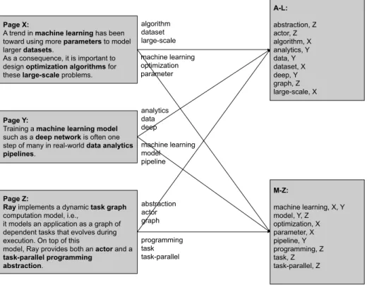
The Bulk Synchronous Parallel (BSP) [129] model became very popular in the early days of the world wide web to crawl websites and process large amounts of data e.g. for building a search index. Implementations like MapReduce [33] or Hadoop [135] made it possible to run programs at a massive scale on cheap commodity hardware, without having to worry about faults. The programming model allows for a simple implementation, but is fairly restrictive. The program logic often has to be completely re-thought to adapt programs to this paradigm. In Fig. 2.2 we show how an inverted index can be built in MapReduce: In this example we have three mappers (one for page X, one for page Y and one for page Z) and two reducers (one for keys from A to L and one for keys from M to Z). Each mapper splits its document into tokens and classifies each of them according to whether they should be entered into the index or not. It then attaches the page to the token and sends all tokens with first letter in A-L to the first reducer and each token with first letter in M-Z to the second reducer. The reducers collect the tokens from each mapper, sort them and combine them into the inverted index.

The implementation in a system like Spark [137] is relatively easy, see the following code snippet. In the first two lines, we iterate through every document, convert it to lower case, split it into tokens and attach the document identifier to each token. In the third line, we then concatenate all the document identifiers corresponding to each token.

rdd.flatMap(lambda (document, contents):

[(token, [document]) for token in contents.lower().split()]) .reduceByKey(lambda a, b: a+b)

By chaining several such MapReduce phases together, we can express iterative compu-tation in this model. By tracking the lineage of the compucompu-tation, this model can be made fault tolerant [139]. This computation model is however fairly restrictive. It does not sup-port state and makes it hard to parallelize applications that cannot naturally be decomposed

(20)

Page X:

A trend in machine learning has been toward using more parameters to model larger datasets.

As a consequence, it is important to design optimization algorithms for these large-scale problems.

Page Y:

Training a machine learning model such as a deep network is often one step of many in real-world data analytics pipelines.

Page Z:

Ray implements a dynamic task graph computation model, i.e.,

it models an application as a graph of dependent tasks that evolves during execution. On top of this

model, Ray provides both an actor and a task-parallel programming abstraction. A-L: abstraction, Z actor, Z algorithm, X analytics, Y data, Y dataset, X deep, Y graph, Z large-scale, X algorithm dataset large-scale M-Z: machine learning, X, Y model, Y, Z optimization, X parameter, X pipeline, Y programming, Z task, Z task-parallel, Z machine learning optimization parameter analytics data deep machine learning model pipeline abstraction actor graph programming task task-parallel

Figure 2.1: Building an inverted index with MapReduce

into a series of map reduce phases. While machine learning training can be expressed in this model [35], performance and flexibility requirements, e.g. for model parallel training, lead us to consider a generalization of the BSP model, the task parallel model.

2.2

The Task Parallel Model

The task parallel model allows the execution of arbitrary side-effect free functions in a distributed way. Each function has input arguments and produces outputs. As soon as all the inputs of a function are available, the function can run on one of the processors and produce its outputs, which will then itself trigger the computation of all functions that depend on these outputs. MapReduce computations are a special case of task parallel computations, where each mapper is a function that transforms a data item, and each reducer is a function that takes the transformed data items and combines them into the output. For the general task parallel model, each function can be different and data can be passed arbitrarily between them. In Fig. 2.2 we show how neural network computations are a natural fit for the task parallel model. There is some input data at the bottom, which gets reshaped and input into an affine layer (linear transform plus bias) and transformed with a rectified linear nonlinearity. Afterwards, a second affine layer is applied and the result is

(21)

CHAPTER 2. THE DISTRIBUTED COMPUTATION LANDSCAPE 7

transformed with a softmax nonlinearity. The last function then computes the loss by taking the cross entropy between the result and the ground truth labels.

Figure 2.2: Neural network task graph, source https://www.tensorflow.org/guide/graphs

The main part of this task parallel computation can be expressed in TensorFlow [1] in the following way. The first three lines define the affine layer and the rectified linear nonlinearity. The second three lines define the second affine layer and the last line applies the softmax nonlinearity and computes the loss function.

weights1 = tf.Variable(...) biases1 = tf.Variable(...)

hidden1 = tf.nn.relu(tf.matmul(images, weights1) + biases1) weights2 = tf.Variable(...)

biases2 = tf.Variable(...)

logits = tf.matmul(hidden1, weights2) + biases2

(22)

These programs can be parallelized in distributed TensorFlow by annotating each func-tion invocafunc-tion with a device it shall be executed on. If there are funcfunc-tions that can be executed in parallel (in the above example, all the computations are serial), this can give large speedups. The task parallel programming model is more powerful than the BSP one and more compatible with the way that serial programs are typically expressed. It can be made fault tolerant either by checkpointing or by recording the lineage. However it cannot support state, which is required by many real applications.

2.3

The Communicating Processes Model

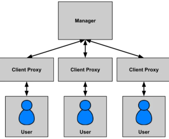
The first distributed computation model we are considering that supports state is commu-nicating processes [53]. It is a generalization of the task parallel model because every task parallel program can be executed on communicating processes by scheduling the functions in the right order onto the processes. There are several realizations of communicating processes, including message passing implementations like MPI [44] or actor systems like Erlang [10], Akka [4] or Orleans [15]. We will focus on actor systems here, because they are as powerful as message passing systems but their programming model is more structured. The actor model was actually formally proposed in the context of artificial intelligence [50]. It models a distributed system as a collection of objects (called actors) that can invoke methods on each other remotely. Each actor has its own state and a mailbox of incoming methods that are invoked on it. Typically, these methods are executed in the order they arrive. Essentially, actors are distributed versions of objects in object oriented programming. As an example for a distributed actor application let us consider a simple chat service (in fact, WhatsApp, one of the widely used chat services is implemented in Erlang)1. The architecture is shown in Fig. 2.3. There is one manager actor that keeps track of the connected users and one client proxy actor per user that forwards messages to the user’s device.

The code is as follows. The listen function takes as an argument the socket that is going to be used for communication with the clients. It starts the manager actor with the spawncall and registers it under the nameclient manager. Then the program accepts new incoming clients with theaccept method. For each new client, a new client proxy is started with spawn in line 9 and it is registered with the manager in 10. The exclamation mark (!) is Erlang’s syntax for sending a message to another actor. In this case, theconnectmessage is sent to client manager with the argument Socket. The manage clients is the main function of the program and the one that the manager actor executes. The state of the actor is in the Sockets argument, it is the list of client sockets. When the manager actor was spawned in line 2, it was initialized as the empty list []. Whenever a new client connects, its socket is added to the list (see line 16), upon termination of the client, it is removed (see line 18). If new data is sent to the manager by one of the clients, it will be forwarded to all other clients in line 20, implemented by the send data function.

(23)

CHAPTER 2. THE DISTRIBUTED COMPUTATION LANDSCAPE 9

Manager

Client Proxy Client Proxy Client Proxy

User User User

Figure 2.3: A chatroom implementation in the actor framework

1 listen(Port) ->

2 Pid = spawn(fun() -> manage_clients([]) end),

3 register(client_manager, Pid),

4 {ok, Listen} = gen_tcp:listen(Port, ?TCP_OPTIONS),

5 accept(Listen).

6

7 accept(Listen) ->

8 {ok, Socket} = gen_tcp:accept(Listen),

9 spawn(fun() -> handle_client(Socket) end),

10 client_manager ! {connect, Socket},

11 accept(Listen).

12

13 manage_clients(Sockets) ->

14 receive

15 {connect, Socket} ->

16 NewSockets = [Socket | Sockets];

17 {disconnect, Socket} ->

18 NewSockets = lists:delete(Socket, Sockets);

19 {data, Data} -> 20 send_data(Sockets, Data), 21 NewSockets = Sockets 22 end, 23 manage_clients(NewSockets). 24 25 send_data(Sockets, Data) ->

(24)

27 lists:foreach(SendData, Sockets).

Note that this example is one very common pattern to write distributed programs, the client server model. It is a special case of communicating processes. In the general case, there is no dedicated server and actors can call methods on each other in arbitrary patterns. Actors can also be made fault tolerant. In Erlang this is done with supervision trees: Actors are organized in a tree and if an actor fails, its parent will be notified and can restart the actor and reset the state [10].

2.4

The Distributed Shared Memory Model

The most powerful distributed programming model is the distributed shared memory model. In an ideal version, it would expose the whole cluster as a single large multicore machine, which can be programmed using multiple execution threads that communicate by reading and writing data from shared memory. In practice this ideal is however not achievable: Latencies of accessing remote memory over the network are typically much larger than latencies of accessing local memory. Therefore if programmers do not take into account the topology of the cluster and just use distributed shared memory in an unstructured fashion, it can lead to very inefficient programs. In addition, distributed shared memory architectures are typically not fault tolerant. However, on specialized supercomputers with special networks, they can lead to very efficient implementations for some workloads. On the cloud, where commodity hardware is typically used, it would be hard to make this programming paradigm successful.

(25)

11

Chapter 3

Motivation: Training Deep Networks

in Spark

Optimization is a crucial step in machine learning. It is very computationally expensive and in many cases has to be executed in a distributed fashion to complete in a reasonable time frame. In the context of machine learning, the optimization problem to solve is to find good parameters for a model given some data by minimizing a loss function. For highly unstructured non-convex problems like optimizing the loss function of a deep neural net-work, first-order optimization algorithms like stochastic gradient descent (SGD) are often the method of choice. We can speed these methods up by distributing the gradient compu-tation over minibatches. This can be quite demanding on the network interconnects because the full model parameters are sent to and from each node in the network on each mini-batch update. In this chapter1, we present an algorithm to run stochastic gradient descent in parallel in the setting where communication is expensive. Instead of communicating the parameters for each minibatch update, we run SGD locally on each node for a few iterations and then average the parameters. While this is a feasible way to train deep neural networks on a slow network, the research performed in this chapter also showed the limitations of data transfer speeds on Spark and served as a motivation to separate the control and data plane for Ray as described in chapter 5.

3.1

Introduction

Deep learning has advanced the state of the art in a number of application domains. Many of the recent advances involve fitting large models (often several hundreds megabytes) to larger datasets (often hundreds of gigabytes). Given the scale of these optimization prob-lems, training can be time-consuming, often requiring multiple days on a single GPU using stochastic gradient descent (SGD). For this reason, much effort has been devoted to

(26)

ing the computational resources of a cluster to speed up the training of deep networks (and more generally to perform distributed optimization).

Many attempts to speed up the training of deep networks rely on asynchronous, lock-free optimization [35, 28]. This paradigm uses the parameter server model [67, 52], in which one or more master nodes hold the latest model parameters in memory and serve them to worker nodes upon request. The nodes then compute gradients with respect to these parameters on a minibatch drawn from the local data shard. These gradients are shipped back to the server, which updates the model parameters.

At the same time, batch-processing frameworks enjoy widespread usage and have been gaining in popularity. Beginning with MapReduce [34], a number of frameworks for dis-tributed computing have emerged to make it easier to write disdis-tributed programs that lever-age the resources of a cluster [141, 57, 88]. These frameworks have greatly simplified many large-scale data analytics tasks. However, state-of-the-art deep learning systems rely on cus-tom implementations to facilitate their asynchronous, communication-intensive workloads. One reason is that popular batch-processing frameworks [34, 141] are not designed to support the workloads of existing deep learning systems. SparkNet implements a scalable, distributed algorithm for training deep networks that lends itself to batch computational frameworks such as MapReduce and Spark and works well out-of-the-box in bandwidth-limited environ-ments.

The benefits of integrating model training with existing batch frameworks are numerous. Much of the difficulty of applying machine learning has to do with obtaining, cleaning, and processing data as well as deploying models and serving predictions. For this reason, it is convenient to integrate model training with the existing data-processing pipelines that have been engineered in today’s distributed computational environments. Furthermore, this ap-proach allows data to be kept in memory from start to finish, whereas a segmented apap-proach requires writing to disk between operations. If a user wishes to train a deep network on the output of a SQL query or on the output of a graph computation and to feed the resulting predictions into a distributed visualization tool, this can be done conveniently within a single computational framework.

We emphasize that the hardware requirements of our approach are minimal. Whereas many approaches to the distributed training of deep networks involve heavy communication (often communicating multiple gradient vectors for every minibatch), our approach gracefully handles the bandwidth-limited setting while also taking advantage of clusters with low-latency communication. For this reason, we can easily deploy our algorithm on clusters that are not optimized for communication. Our implementation works well out-of-the box on a five-node EC2 cluster in which broadcasting and collecting model parameters (several hundred megabytes per worker) takes on the order of 20 seconds, and performing a single minibatch gradient computation requires about 2 seconds (for AlexNet). We achieve this by providing a simple algorithm for parallelizing SGD that involves minimal communication and lends itself to straightforward implementation in batch computational frameworks. Our goal is not to outperform custom computational frameworks but rather to propose a system that can be easily implemented in popular batch frameworks and that performs nearly as

(27)

CHAPTER 3. MOTIVATION: TRAINING DEEP NETWORKS IN SPARK 13

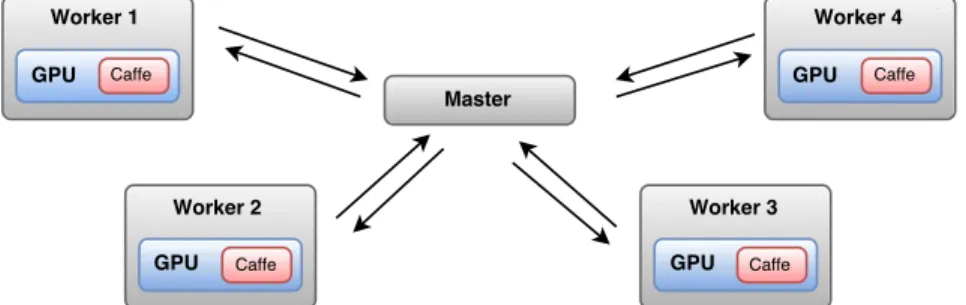
Figure 3.1: This figure depicts the SparkNet architecture.

well as what can be accomplished with specialized frameworks.

3.2

Implementation

Here we describe our implementation of SparkNet. SparkNet builds on Apache Spark [141] and the Caffe deep learning library [58]. In addition, we use Java Native Access for accessing Caffe data and weights natively from Scala, and we use the Java implementation of Google Protocol Buffers to allow the dynamic construction of Caffe networks at runtime.

The Net class wraps Caffe and exposes a simple API containing the methods shown in Listing 3.1. TheNetParamstype specifies a network architecture, and theWeightCollection type is a map from layer names to lists of weights. It allows the manipulation of network components and the storage of weights and outputs for individual layers. To facilitate manip-ulation of data and weights without copying memory from Caffe, we implement theNDArray class, which is a lightweight multi-dimensional tensor library. One benefit of building on Caffe is that any existing Caffe model definition or solver file is automatically compatible

c l a s s Net {

def Net ( n e t P a r a m s : N e t P a r a m s ): Net

def s e t T r a i n i n g D a t a ( d a t a : I t e r a t o r [( NDArray , Int )]) def s e t V a l i d a t i o n D a t a ( d a t a : I t e r a t o r [( NDArray , Int )]) def t r a i n ( n u m S t e p s : Int )

def t e s t ( n u m S t e p s : Int ): F l o a t

def s e t W e i g h t s ( w e i g h t s : W e i g h t C o l l e c t i o n ) def g e t W e i g h t s (): W e i g h t C o l l e c t i o n

}

(28)

val n e t P a r a m s = N e t P a r a m s ( R D D L a y e r (" d a t a " , s h a p e = L i s t ( b a t c h s i z e , 1 , 28 , 28)) , R D D L a y e r (" l a b e l " , s h a p e = L i s t ( b a t c h s i z e , 1)) , C o n v L a y e r (" c o n v 1 " , L i s t (" d a t a ") , k e r n e l =(5 ,5) , n u m F i l t e r s =20) , P o o l L a y e r (" p o o l 1 " , L i s t (" c o n v 1 ") , p o o l = Max , k e r n e l =(2 ,2) , s t r i d e =(2 ,2)) , C o n v L a y e r (" c o n v 2 " , L i s t (" p o o l 1 ") , k e r n e l =(5 ,5) , n u m F i l t e r s =50) , P o o l L a y e r (" p o o l 2 " , L i s t (" c o n v 2 ") , p o o l = Max , k e r n e l =(2 ,2) , s t r i d e =(2 ,2)) , L i n e a r L a y e r (" ip1 " , L i s t (" p o o l 2 ") , n u m O u t p u t s =500) , A c t i v a t i o n L a y e r (" r e l u 1 " , L i s t (" ip1 ") , a c t i v a t i o n = R e L U ) , L i n e a r L a y e r (" ip2 " , L i s t (" r e l u 1 ") , n u m O u t p u t s =10) , S o f t m a x W i t h L o s s (" l o s s " , L i s t (" ip2 " , " l a b e l ")) )

Listing 3.2: Example network specification in SparkNet

with SparkNet. There is a large community developing Caffe models and extensions, and these can easily be used in SparkNet. By building on top of Spark, we inherit the advantages of modern batch computational frameworks. These include the high-throughput loading and preprocessing of data and the ability to keep data in memory between operations. In List-ing 3.2, we give an example of how network architectures can be specified in SparkNet. In addition, model specifications or weights can be loaded directly from Caffe files. An example sketch of code that uses our API to perform distributed training is given in Listing 3.3.

Parallelizing SGD

To perform well in bandwidth-limited environments, we recommend a parallelization scheme for SGD that requires minimal communication. This approach is not specific to SGD. Indeed, SparkNet works out of the box with any Caffe solver.

The parallelization scheme is described in Listing 3.3. Spark consists of a single master node and a number of worker nodes. The data is split among the Spark workers. In every iteration, the Spark master broadcasts the model parameters to each worker. Each worker then runs SGD on the model with its subset of data for a fixed number of iterations τ (we use τ = 50 in Listing 3.3) or for a fixed length of time, after which the resulting model parameters on each worker are sent to the master and averaged to form the new model parameters. We recommend initializing the network by running SGD for a small number of iterations on the master. A similar and more sophisticated approach to parallelizing SGD with minimal communication overhead is discussed in [142].

(29)

CHAPTER 3. MOTIVATION: TRAINING DEEP NETWORKS IN SPARK 15

var t r a i n D a t a = l o a d D a t a ( . . . )

var t r a i n D a t a = p r e p r o c e s s ( t r a i n D a t a ). c a c h e () var n e t s = t r a i n D a t a . f o r e a c h P a r t i t i o n ( d a t a = > {

var net = Net ( n e t P a r a m s ) net . s e t T r a i n i n g D a t a ( d a t a ) net )

var w e i g h t s = i n i t i a l W e i g h t s ( . . . ) for ( i < - 1 to 1 0 0 0 ) {

var b r o a d c a s t W e i g h t s = b r o a d c a s t ( w e i g h t s )

n e t s . map ( net = > net . s e t W e i g h t s ( b r o a d c a s t W e i g h t s . v a l u e )) w e i g h t s = n e t s . map ( net = > {

net . t r a i n ( 5 0 )

// an a v e r a g e of W e i g h t C o l l e c t i o n o b j e c t s net . g e t W e i g h t s ( ) } ) . m e a n ()

}

Listing 3.3: Distributed training example

and collecting model parameters (hundreds of megabytes per worker and gigabytes in total) after every SGD update, which occurs tens of thousands of times during training. On our EC2 cluster, each broadcast and collection takes about twenty seconds, putting a bound on the speedup that can be expected using this approach without better hardware or without partitioning models across machines. Our approach broadcasts and collects the parameters a factor of τ times less for the same number of iterations. In our experiments, we setτ = 50, but other values seem to work about as well.

We note that Caffe supports parallelism across multiple GPUs within a single node. This is not a competing form of parallelism but rather a complementary one. In some of our experiments, we use Caffe to handle parallelism within a single node, and we use the parallelization scheme described in Listing 3.3 to handle parallelism across nodes.

3.3

Experiments

In Section 3.3, we will benchmark the performance of SparkNet and measure the speedup that our system obtains relative to training on a single node. However, the outcomes of those experiments depend on a number of different factors. In addition to τ (the number of iterations between synchronizations) and K (the number of machines in our cluster), they depend on the communication overhead in our clusterS. In Section 3.3, we find it instructive to measure the speedup in the idealized case of zero communication overhead(S = 0). This idealized model gives us an upper bound on the maximum speedup that we could hope to

(30)

obtain in a real-world cluster, and it allows us to build a model for the speedup as a function of S (the overhead is easily measured in practice).

Theoretical Considerations

Before benchmarking our system, we determine the maximum possible speedup that could be obtained in principle in a cluster with no communication overhead. We determine the dependence of this speedup on the parametersτ (the number of iterations between synchro-nizations) and K (the number of machines in our cluster).

Limitations of Naive Parallelization

To begin with, we consider the theoretical limitations of a naive parallelism scheme which parallelizes SGD by distributing each minibatch computation over multiple machines (see Figure 3.2b). Let Na(b) be the number of serial iterations of SGD required to obtain an

accuracy of a when training with a batch size of b (when we say accuracy, we are referring to test accuracy). Suppose that computing the gradient over a batch of size b requires C(b) units of time. Then the running time required to achieve an accuracy ofawith serial training is

Na(b)C(b). (3.1)

A naive parallelization scheme attempts to distribute the computation at each iteration by dividing each minibatch between the K machines, computing the gradients separately, and aggregating the results on one node. Under this scheme, the cost of the computation done on a single node in a single iteration is C(b/K) and satisfiesC(b/K)≥C(b)/K (the cost is sublinear in the batch size). In a system with no communication overhead and no overhead for summing the gradients, this approach could in principle achieve an accuracy ofa in time

Na(b)C(b)/K. This represents a linear speedup in the number of machines (for values of K

up to the batch size b).

In practice, there are several important considerations. First, for the approximation

C(b/K) ≈ C(b)/K to hold, K must be much smaller than b, limiting the number of ma-chines we can use to effectively parallelize the minibatch computation. One might imagine circumventing this limitation by using a larger batch sizeb. Unfortunately, the benefit of us-ing larger batches is relatively modest. As the batch sizeb increases,Na(b) does not decrease

enough to justify the use of a very large value of b.

Furthermore, the benefits of this approach depend greatly on the degree of communication overhead. If aggregating the gradients and broadcasting the model parameters requires S

units of time, then the time required by this approach is at least C(b)/K+S per iteration and Na(b)(C(b)/K+S) to achieve an accuracy of a. Therefore, the maximum achievable

speedup is C(b)/(C(b)/K +S) ≤ C(b)/S. We may expect S to increase modestly as K

(31)

CHAPTER 3. MOTIVATION: TRAINING DEEP NETWORKS IN SPARK 17

Limitations of SparkNet Parallelization

The performance of the naive parallelization scheme is easily understood because its behavior is equivalent to that of the serial algorithm. In contrast, SparkNet uses a parallelization scheme that is not equivalent to serial SGD (described in Section 3.2), and so its analysis is more complex.

SparkNet’s parallelization scheme proceeds in rounds (see Figure 3.2c). In each round, each machine runs SGD for τ iterations with batch size b. Between rounds, the models on the workers are gathered together on the master, averaged, and broadcast to the workers.

We use M_a(b, K, τ) to denote the number of rounds required to achieve an accuracy ofa. The number of parallel iterations of SGD under SparkNet’s parallelization scheme required to achieve an accuracy ofa is thenτ Ma(b, K, τ), and the wallclock time is

(τ C(b) +S)M_a(b, K, τ), (3.2)

where S is the time required to gather and broadcast model parameters.

To measure the sensitivity of SparkNet’s parallelization scheme to the parameters τ and

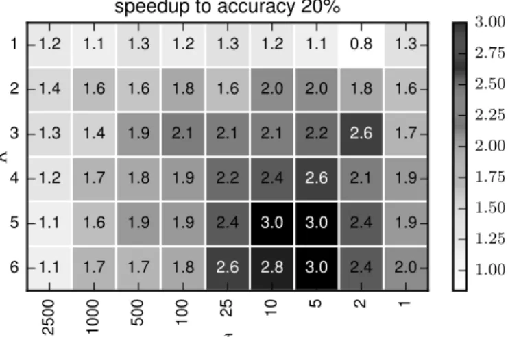
K, we consider a grid of values of K and τ. For each pair of parameters, we run SparkNet using a modified version of AlexNet on a subset of ImageNet (the first 100 classes each with approximately 1000 data points) for a total of 20000 parallel iterations. For each of these training runs, we compute the ratio τ Ma(b, K, τ)/Na(b). This is the speedup achieved

relative to training on a single machine whenS = 0. In Figure 3.3, we plot a heatmap of the speedup given by the SparkNet parallelization scheme under different values of τ and K.

Figure 3.3 exhibits several trends. The top row of the heatmap corresponds to the case

K = 1, where we use only one worker. Since we do not have multiple workers to synchronize when K = 1, the number of iterations τ between synchronizations does not matter, so all of the squares in the top row of the grid should behave similarly and should exhibit a speedup factor of 1 (up to randomness in the optimization). The rightmost column of each heatmap corresponds to the case τ = 1, where we synchronize after every iteration of SGD. This is equivalent to running serial SGD with a batch size of Kb, where b is the batchsize on each worker (in these experiments we useb = 100). In this column, the speedup should increase sublinearly with K. We note that it is slightly surprising that the speedup does not increase monotonically from left to right as τ decreases. Intuitively, we might expect more synchronization to be strictly better (recall we are disregarding the overhead due to synchronization). However, our experiments suggest that modest delays between synchronizations can be beneficial.

This experiment capture the speedup that we can expect from the SparkNet paralleliza-tion scheme in the case of zero communicaparalleliza-tion overhead (the numbers are dataset specific, but the trends are of interest). Having measured these numbers, it is straightforward to compute the speedup that we can expect as a function of the communication overhead.

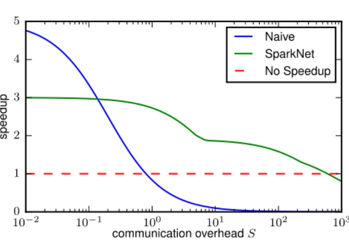
In Figure 3.4, we plot the speedup expected both from naive parallelization and from SparkNet on a five-node cluster as a function of S (normalized so that C(b) = 1). As ex-pected, naive parallelization gives a maximum speedup of 5 (on a five-node cluster) when

(32)

there is zero communication overhead (note that our plot does not go all the way toS = 0), and it gives no speedup when the communication overhead is comparable to or greater than the cost of a minibatch computation. In contrast, SparkNet gives a relatively consistent speedup even when the communication overhead is 100 times the cost of a minibatch com-putation.

The speedup given by the naive parallelization scheme can be computed exactly and is given by C(b)/(C(b)/K +S). This formula is essentially Amdahl’s law. Note that when

S ≥ C(b), the naive parallelization scheme is slower than the computation on a single machine. The speedup obtained by SparkNet is Na(b)C(b)/[(τ C(b) +S)Ma(b, K, τ)] for a

specific value ofτ. The numerator is the time required by serial SGD to achieve an accuracy of a from Equation 3.1, and the denominator is the time required by SparkNet to achieve the same accuracy from Equation 3.2. Choosing the optimal value ofτ gives us a speedup of maxτNa(b)C(b)/[(τ C(b) +S)Ma(b, K, τ)]. In practice, choosing τ is not a difficult problem.

The ratioNa(b)/(τ Ma(b, K, τ)) (the speedup whenS = 0) degrades slowly as τ increases, so

it suffices to chooseτ to be a small multiple of S (say 5S) so that the algorithm spends only a fraction of its time in communication.

When plotting the SparkNet speedup in Figure 3.4, we do not maximize over all positive integer values ofτ but rather over the setτ ∈ {1,2,5,10,25,100,500,1000,2500}, and we use the values of Na(b) and Ma(b, K, τ) corresponding to the fifth row of Figure 3.3. Including

more values of τ would only increase the SparkNet speedup. The distributed training of deep networks is typically thought of as a communication-intensive procedure. However, Figure 3.4 demonstrates the value of SparkNet’s parallelization scheme even in the most bandwidth-limited settings.

The naive parallelization scheme may appear to be a straw man. However, it is a frequently-used approach to parallelizing SGD [95, 55], especially when asynchronous up-dates are not an option (as in computational frameworks like MapReduce and Spark).

Training Benchmarks

To explore the scaling behavior of our algorithm and implementation, we perform experi-ments on EC2 using clusters of g2.8xlarge nodes. Each node has four NVIDIA GRID GPUs and 60GB memory. We train the default Caffe model of AlexNet [63] on the ImageNet dataset [108]. We run SparkNet with K = 3, 5, and 10 and plot the results in Figure 3.5. For comparison, we also run Caffe on the same cluster with a single GPU and no commu-nication overhead to obtain the K = 1 plot. These experiments use only a single GPU on each node. To measure the speedup, we compare the wall-clock time required to obtain an accuracy of 45%. With 1 GPU and no communication overhead, this takes 55.6 hours. With 3, 5, and 10 GPUs, SparkNet takes 22.9, 14.5, and 12.8 hours, giving speedups of 2.4, 3.8, and 4.4.

We also train the default Caffe model of GoogLeNet [124] on ImageNet. We run SparkNet with K = 3 and K = 6 and plot the results in Figure 3.6. In these experiments, we use Caffe’s multi-GPU support to take advantage of all four GPUs within each node, and we use

(33)

CHAPTER 3. MOTIVATION: TRAINING DEEP NETWORKS IN SPARK 19

SparkNet’s parallelization scheme to handle parallelism across nodes. For comparison, we train Caffe on a single node with four GPUs and no communication overhead. To measure the speedup, we compare the wall-clock time required to obtain an accuracy of 40%. Relative to the baseline of Caffe with four GPUs, SparkNet on 3 and 6 nodes gives speedups of 2.7 and 3.2. Note that this is on top of the speedup of roughly 3.5 that Caffe with four GPUs gets over Caffe with one GPU, so the speedups that SparkNet obtains over Caffe on a single GPU are roughly 9.4 and 11.2.

Furthermore, we explore the dependence of the parallelization scheme described in Sec-tion 3.2 on the parameter τ which determines the number of iterations of SGD that each worker does before synchronizing with the other workers. These results are shown in Fig-ure 3.7. Note that in the presence of stragglers, it suffices to replace the fixed number of iterations τ with a fixed length of time, but in our experimental setup, the timing was suf-ficiently consistent and stragglers did not arise. The single GPU experiment in Figure 3.5 was trained on a single GPU node with no communication overhead.

3.4

Related Work

Much work has been done to build distributed frameworks for training deep networks. [29] build a model-parallel system for training deep networks on a GPU cluster using MPI over Infiniband. [35] build DistBelief, a distributed system capable of training deep networks on thousands of machines using stochastic and batch optimization procedures. In particular, they highlight asynchronous SGD and batch L-BFGS. Distbelief exploits both data paral-lelism and model paralparal-lelism. [28] build Project Adam, a system for training deep networks on hundreds of machines using asynchronous SGD. [67, 52] build parameter servers to exploit model and data parallelism, and though their systems are better suited to sparse gradient updates, they could very well be applied to the distributed training of deep networks. More recently, [75] build TensorFlow, a sophisticated system for training deep networks and more generally for specifying computation graphs and performing automatic differentiation. [55] build FireCaffe, a data-parallel system that achieves impressive scaling using naive paral-lelization in the high-performance computing setting. They minimize communication over-head by using a tree reduce for aggregating gradients in a supercomputer with Cray Gemini interconnects.

These custom systems have numerous advantages including high performance, fine-grained control over scheduling and task placement, and the ability to take advantage of low-latency communication between machines. On the other hand, due to their demanding communi-cation requirements, they are unlikely to exhibit the same scaling on an EC2 cluster. Fur-thermore, due to their nature as custom systems, they lack the benefits of tight integration with general-purpose computational frameworks such as Spark. For some of these systems, preprocessing must be done separately by a MapReduce style framework, and data is written to disk between segments of the pipeline. With SparkNet, preprocessing and training are both done in Spark.

(34)

Training a machine learning model such as a deep network is often one step of many in real-world data analytics pipelines [121]. Obtaining, cleaning, and preprocessing the data are often expensive operations, as is transferring data between systems. Training data for a machine learning model may be derived from a streaming source, from a SQL query, or from a graph computation. A user wishing to train a deep network in a custom system on the output of a SQL query would need a separate SQL engine. In SparkNet, training a deep network on the output of a SQL query, or a graph computation, or a streaming data source is straightforward due to its general purpose nature and its support for SQL, graph computations, and data streams [9, 47, 138].

Some attempts have been made to train deep networks in general-purpose computational frameworks, however, existing work typically hinges on extremely low-latency intra-cluster communication. [95] train deep networks in Spark on top of YARN using SGD and leverage cluster resources to parallelize the computation of the gradient over each minibatch. To achieve competitive performance, they use remote direct memory accesses over Infiniband to exchange model parameters quickly between GPUs. In contrast, SparkNet tolerates low-bandwidth intra-cluster communication and works out of the box on Amazon EC2.

A separate line of work addresses speeding up the training of deep networks using single-machine parallelism. For example, Caffe con Troll [49] modifies Caffe to leverage both CPU and GPU resources within a single node. These approaches are compatible with SparkNet and the two can be used in conjunction.

Many popular computational frameworks provide support for training machine learning models [76] such as linear models and matrix factorization models. However, due to the demanding communication requirements and the larger scale of many deep learning problems, these libraries have not been extended to include deep networks.

Various authors have studied the theory of averaging separate runs of SGD. In the bandwidth-limited setting, [144] analyze a simple algorithm for convex optimization that is easily implemented in the MapReduce framework and can tolerate high-latency commu-nication between machines. [142] define a parallelization scheme that penalizes divergences between parallel workers, and they provide an analysis in the convex case. [143] propose a general abstraction for parallelizing stochastic optimization algorithms along with a Spark implementation.

3.5

Discussion

We have described an approach to distributing the training of deep networks in communication-limited environments that lends itself to an implementation in batch computational frame-works like MapReduce and Spark. We provide SparkNet, an easy-to-use deep learning im-plementation for Spark that is based on Caffe and enables the easy parallelization of existing Caffe models with minimal modification. As machine learning increasingly depends on larger and larger datasets, integration with a fast and general engine for big data processing such as Spark allows researchers and practitioners to draw from a rich ecosystem of tools to develop

(35)

CHAPTER 3. MOTIVATION: TRAINING DEEP NETWORKS IN SPARK 21

and deploy their models. They can build models that incorporate features from a variety of data sources like images on a distributed file system, results from a SQL query or graph database query, or streaming data sources.

Using a smaller version of the ImageNet benchmark we quantify the speedup achieved by SparkNet as a function of the size of the cluster, the communication frequency, and the cluster’s communication overhead. We demonstrate that our approach is effective even in highly bandwidth-limited settings. On the full ImageNet benchmark we showed that our system achieves a sizable speedup over a single node experiment even with few GPUs.

The code for SparkNet is available at https://github.com/amplab/SparkNet. We in-vite contributions and hope that the project will help bring a diverse set of deep learning applications to the Spark community.

(36)

(a) This figure depicts a serial run of SGD. Each block corresponds to a single SGD

update with batch size b. The quantity Na(b) is the number of iterations required to

achieve an accuracy of a.

(b) This figure depicts a parallel run of SGD onK = 4 machines under a naive

paralleliza-tion scheme. At each iteraparalleliza-tion, each batch of size b is divided among the K machines,

the gradients over the subsets are computed separately on each machine, the updates are aggregated, and the new model is broadcast to the workers. Algorithmically, this approach is exactly equivalent to the serial run of SGD in Figure 3.2a and so the number of iterations required to achieve an accuracy ofais the same value Na(b).

(c) This figure depicts a parallel run of SGD on K = 4 machines under SparkNet’s

parallelization scheme. At each step, each machine runs SGD with batch size b for

τ iterations, after which the models are aggregated, averaged, and broadcast to the

workers. The quantity Ma(b, K, τ) is the number of rounds (of τ iterations) required to

obtain an accuracy ofa. The total number of parallel iterations of SGD under SparkNet’s

parallelization scheme required to obtain an accuracy ofais then τ Ma(b, K, τ).

(37)

CHAPTER 3. MOTIVATION: TRAINING DEEP NETWORKS IN SPARK 23 2500 1000 500 100 25 10 5 2 1 τ 6 5 4 3 2 1 K 1.1 1.7 1.7 1.8 2.6 2.8 3.0 2.4 2.0 1.1 1.6 1.9 1.9 2.4 3.0 3.0 2.4 1.9 1.2 1.7 1.8 1.9 2.2 2.4 2.6 2.1 1.9 1.3 1.4 1.9 2.1 2.1 2.1 2.2 2.6 1.7 1.4 1.6 1.6 1.8 1.6 2.0 2.0 1.8 1.6 1.2 1.1 1.3 1.2 1.3 1.2 1.1 0.8 1.3 speedup to accuracy 20% 1.00 1.25 1.50 1.75 2.00 2.25 2.50 2.75 3.00

Figure 3.3: This figure shows the speedup τ Ma(b, τ, K)/Na(b) given by SparkNet’s

paral-lelization scheme relative to training on a single machine to obtain an accuracy of a= 20%. Each grid square corresponds to a different choice of K and τ. We show the speedup in the zero communication overhead setting. This experiment uses a modified version of AlexNet on a subset of ImageNet (100 classes each with approximately 1000 images). Note that these numbers are dataset specific. Nevertheless, the trends they capture are of interest.

(38)

10−2 ₁₀−1 ₁₀0 ₁₀1 ₁₀2 ₁₀3 communication overheadS 0 1 2 3 4 5 speedup Naive SparkNet No Speedup

Figure 3.4: This figure shows the speedups obtained by the naive parallelization scheme and by SparkNet as a function of the cluster’s communication overhead (normalized so that

C(b) = 1). We consider K = 5. The data for this plot applies to training a modified version of AlexNet on a subset of ImageNet (approximately 1000 images for each of the first 100 classes). The speedup obtained by the naive parallelization scheme is C(b)/(C(b)/K+S). The speedup obtained by SparkNet isN_a(b)C(b)/[(τ C(b) +S)M_a(b, K, τ)] for a specific value ofτ. The numerator is the time required by serial SGD to achieve an accuracy of a, and the denominator is the time required by SparkNet to achieve the same accuracy (see Equation 3.1 and Equation 3.2). For the optimal value of τ, the speedup is maxτNa(b)C(b)/[(τ C(b) +

S)Ma(b, K, τ)]. To plot the SparkNet speedup curve, we maximize over the set of values

τ ∈ {1,2,5,10,25,100,500,1000,2500} and use the values Ma(b, K, τ) and Na(b) from the

experiments in the fifth row of Figure 3.3. In our experiments, we have S ≈ 20s and

(39)

CHAPTER 3. MOTIVATION: TRAINING DEEP NETWORKS IN SPARK 25 0 5 10 15 20 hours 05 10 15 20 25 30 35 4045

accuracy CaffeSparkNet 3 node SparkNet 5 node SparkNet 10 node

Figure 3.5: This figure shows the perfor-mance of SparkNet on a 3-node, 5-node, and 10-node cluster, where each node has 1 GPU. In these experiments, we use τ = 50. The baseline was obtained by running Caffe on a single GPU with no communication. The experiments are performed on Ima-geNet using AlexNet.

0 20 40 60 80 100 120 hours 0 10 20 30 40 50 60

accuracy Caffe 4 GPU

SparkNet 3 node 4 GPU SparkNet 6 node 4 GPU

Figure 3.6: This figure shows the perfor-mance of SparkNet on a 3-node cluster and on a 6-node cluster, where each node has 4 GPUs. In these experiments, we use

τ = 50. The baseline uses Caffe on a single node with 4 GPUs and no communication overhead. The experiments are performed on ImageNet using GoogLeNet.

0

2

4

6

8

10

hours

0

5

10

15

20

25

30

35

40

45

accuracy

20 iterations

50 iterations

100 iterations

150 iterations

Figure 3.7: This figure shows the dependence of the parallelization scheme described in Section 3.2 on τ. Each experiment was run with K = 5 workers. This figure shows that good performance can be achieved without collecting and broadcasting the model after every SGD update.

(40)

Chapter 4

The System Requirements

As we have already seen in chapter 2, there are many different programming models for distributed computing. In this chapter1 we study the requirements of a general purpose dis-tributed system that can support emerging artificial intelligence applications like reinforce-ment learning both in terms of the programming model and the system implereinforce-mentation.

The landscape of machine learning (ML) applications is undergoing a significant change. While ML has predominantly focused on training and serving predictions based on static models (Figure 4.1a), there is now a strong shift toward the tight integration of ML mod-els in feedback loops. Indeed, ML applications are expanding from the supervised learning paradigm, in which static models are trained on offline data, to a broader paradigm, ex-emplified by reinforcement learning (RL), in which applications may operate in real envi-ronments, fuse and react to sensory data from numerous input streams, perform continuous micro-simulations, and close the lo