Feature selection and hierarchical
classifier design with applications to
human motion recognition
by
Cecille Freeman
A thesis
presented to the University of Waterloo in fulfillment of the
thesis requirement for the degree of Doctor of Philosophy
in
Electrical and Computer Engineering
Waterloo, Ontario, Canada, 2014
c
I hereby declare that I am the sole author of this thesis. This is a true copy of the thesis, including any required final revisions, as accepted by my examiners.
Abstract
The performance of a classifier is affected by a number of factors including classifier type, the input features and the desired output. This thesis examines the impact of feature selection and classification problem division on classification accuracy and complexity.
Proper feature selection can reduce classifier size and improve classifier performance by minimizing the impact of noisy, redundant and correlated features. Noisy features can cause false association between the features and the classifier output. Redundant and correlated features increase classifier complexity without adding additional information.
Output selection or classification problem division describes the division of a large clas-sification problem into a set of smaller problems. Problem division can improve accuracy by allocating more resources to more difficult class divisions and enabling the use of more specific feature sets for each sub-problem.
The first part of this thesis presents two methods for creating feature-selected hierarchi-cal classifiers. The feature-selected hierarchihierarchi-cal classification method jointly optimizes the features and classification tree-design using genetic algorithms. The multi-modal binary tree (MBT) method performs the class division and feature selection sequentially and tol-erates misclassifications in the higher nodes of the tree. This yields a piecewise separation for classes that cannot be fully separated with a single classifier. Experiments show that the accuracy of MBT is comparable to other multi-class extensions, but with lower test time. Furthermore, the accuracy of MBT is significantly higher on multi-modal data sets. The second part of this thesis focuses on input feature selection measures. A number of filter-based feature subset evaluation measures are evaluated with the goal of assessing their performance with respect to specific classifiers. Although there are many feature selection measures proposed in literature, it is unclear which feature selection measures are appropriate for use with different classifiers. Sixteen common filter-based measures are tested on 20 real and 20 artificial data sets, which are designed to probe for specific feature selection challenges. The strengths and weaknesses of each measure are discussed with respect to the specific feature selection challenges in the artificial data sets, correlation with classifier accuracy and their ability to identify known informative features.
The results indicate that the best filter measure is classifier-specific. K-nearest neigh-bours classifiers work well with subset-based RELIEF, correlation feature selection or con-ditional mutual information maximization, whereas Fisher’s interclass separability criterion and conditional mutual information maximization work better for support vector machines. Based on the results of the feature selection experiments, two new filter-based measures are proposed based on conditional mutual information maximization, which performs well
but cannot identify dependent features in a set and does not include a check for corre-lated features. Both new measures explicitly check for dependent features and the second measure also includes a term to discount correlated features. Both measures correctly iden-tify known informative features in the artificial data sets and correlate well with classifier accuracy.
The final part of this thesis examines the use of feature selection for time-series data by using feature selection to determine important individual time windows or key frames in the series. Time-series feature selection is used with the MBT algorithm to create classification trees for time-series data. The feature selected MBT algorithm is tested on two human motion recognition tasks: full-body human motion recognition from joint angle data and hand gesture recognition from electromyography data. Results indicate that the feature selected MBT is able to achieve high classification accuracy on the time-series data while maintaining a short test time.
Acknowledgements
Fist and foremost I would like to thank my supervisors, Dr. Dana Kuli´c and Dr.
Otman Basir. Dr. Basir, our discussions were always interesting and challenging your encouragement to constantly push forward in the research benefited this thesis greatly.
Dr. Kuli´c, our discussions were always enlightening and informative, exposing me to
different problems and research areas that I had not previously considered. Your personal commitment to your students is amazing. You were at every meeting, read every paper and responded to every email. I am so very grateful for all of your support.
Thank you to my committee members for their careful consideration of this thesis and their many insightful comments. Thanks also to the ECE administrative staff for all of your help setting up the defense and getting this thesis completed.
Each week, our lab would meet for a discussion of our ongoing research and other work in our fields. The discussions we had both inside and outside of these meetings were always so interesting. I loved hearing about all your research and am so grateful for your many new perspectives and insights.
I have always found teaching to be extremely enjoyable and the courses I TA’d at the University of Waterloo were no exception. This is in no small part due to the excellent instructors, Dr. Hiren Patel and Dr. Fakhri Karray, and my co-TA Jamil.
Thanks to Dr. Areibi and Dr. Dony for convincing me to do this PhD in the first place. This project was made possible by the numerous grants and scholarships, including grants from the National Science and Engineering Research Council (NSERC), the Ontario Graduate Scholarship program (OGS), grants from the University of Waterloo and the the facilities of the Shared Hierarchical Academic Research Computing Network (SHARC-NET:www.sharcnet.ca) and Compute/Calcul Canada. Thanks also to Thalmic Labs Inc. for allowing us to work with their prototype data and for the numerous helpful meetings. Not all of the people I need to thank made research contributions to this thesis. My amazing friends kept me sane during this whole crazy endeavor. My party in crime: Morri, Meghan, Alicia and Heather. You guys are amazing for so many reasons. Thanks to Lish, Kev, Alex, James, Pymer, Ashley, Alana, Dom, Kyle and the rest of you crazies for a good night out every once in a while. Thanks to the old grad crew: Anna, who managed to get out, and Zoe, who did not. Thank you Danny, for generally being amazing and for showing me that it is actually possible to complete one of these things.
A big, gigantic, huge thanks to the tipsters, fly by night and all the WODS people. I swear that at some points ultimate was the only thing keeping me from losing it completely.
Lastly, thanks to my amazing family. Lily and Tooty, who were always supportive of everything I did. Mark and Drew and my crazy cousins for making the many trips to Toronto so much easier. To my new in-law family for being so great and accepting. Thanks to my brother Jacob for being a younger, more fun version of me. Thanks to my parents for being amazing and supportive and pretending like I made sense when I was talking about my research. Lastly, thanks to Jon for agreeing to put up with my particular brand of crazy for this long.
Dedication
This thesis is dedicated to Jon, who knows the best way to show someone you love them is to dedicate a gigantic, academic tome to them.
Table of Contents
List of Tables xiii
List of Figures xix
Acronyms xxiii
Glossary xxvii
1 Introduction 1
2 Previous Work 5
2.1 Notation . . . 5
2.2 Feature Selection and Feature extraction . . . 5
2.3 Feature extraction techniques . . . 7
2.3.1 Properties of feature extraction techniques . . . 7
2.3.2 Variance-based feature extraction techniques . . . 10
2.3.3 Distance-based feature extraction techniques . . . 13
2.3.4 Neighbourhood graph-based feature extraction techniques . . . 15
2.3.5 Independent Component Analysis (ICA) for feature extraction . . . 17
2.3.6 Feature extraction techniques based on clustering . . . 18
2.3.7 Autoencoders for feature extraction . . . 19
2.3.9 Domain specific feature extraction . . . 19
2.4 Feature selection techniques . . . 20
2.4.1 Properties . . . 21
2.4.2 Feature subset evaluation measures . . . 23
2.4.3 Feature set selection techniques . . . 32
2.5 Hierarchical classifiers and multi-class extensions for binary classifiers . . . 38
2.5.1 One vs. rest . . . 38
2.5.2 Fuzzy one vs. rest. . . 39
2.5.3 One vs. one . . . 40
2.5.4 DAG-SVM . . . 40
2.5.5 Hierarchical classifiers . . . 40
2.5.6 Comparison . . . 42
2.6 Algorithms used in this work . . . 43
2.6.1 Support Vector Machines (SVM) . . . 43
2.6.2 K-nearest neighbours (KNN). . . 45
2.6.3 Genetic algorithms . . . 45
2.6.4 K-means clustering . . . 47
2.7 Human motion recognition . . . 48
2.8 Summary . . . 50
3 Hierarchical Classifier Design 52 3.1 Feature-selected hierarchical classifier (FSHC) . . . 53
3.1.1 Feature Selected Hierarchical Classifier Design . . . 54
3.1.2 Experiments . . . 62
3.1.3 Results and Discussion . . . 67
3.1.4 FSHC Summary . . . 84
3.2 Multi-modal binary-tree classification (MBT) . . . 86
3.2.2 Results and Discussion . . . 92
3.2.3 MBT Summary . . . 100
3.3 Summary . . . 101
4 Evaluation of filter based feature selection measures 103 4.1 Filter measures . . . 104
4.2 Experiments . . . 104
4.2.1 Data Sets . . . 107
4.2.2 Combining univariate and additive multivariate measures . . . 108
4.3 Results and Discussion . . . 112
4.3.1 Ability of filter measures to identify informative features . . . 112
4.3.2 Correlation of filter measures with classifier accuracy . . . 113
4.3.3 A note on the Monk 2 data set . . . 129
4.3.4 Parameter sensitivity . . . 131
4.3.5 Summary of filter measure evaluation . . . 142
4.4 Proposal for a new filter measure . . . 148
4.4.1 Experiments . . . 152
4.4.2 Results and discussion . . . 152
4.5 Summary . . . 153
5 Feature Selection for time-series human-motion data 156 5.1 Full body motion recognition from joint angles . . . 158
5.1.1 Experiments . . . 159
5.1.2 Results and Discussion . . . 162
5.2 Hand gesture recognition from Electromyography (EMG) sensor data . . . 174
5.2.1 Experiments . . . 178
5.2.2 Results and Discussion . . . 188
6 Conclusions 197
6.1 Future Work . . . 199
6.1.1 Tree-based classifiers . . . 199
6.1.2 Dependent features . . . 200
6.1.3 EMG hand gesture classification . . . 200
6.1.4 Application to other domains . . . 203
APPENDICES 205 A Classifier accuracy on tested data sets 206 B Filter measure correlation values 210 B.1 RELIEF-based measures . . . 210
B.2 Probability-based measures . . . 215
B.3 Mutual Information measures . . . 225
B.3.1 Univariate measures . . . 225 B.3.2 Multivariate measures . . . 229 B.4 Consistency . . . 235 B.5 Laplacian score . . . 237 B.6 MCFS . . . 243 B.7 CFS . . . 251
C Performance of filter measures on the artificial data sets 253 C.1 Binary data sets. . . 253
C.2 Monk 1 and Monk 3 . . . 255
C.3 Monk 2 . . . 256
C.4 Simple dependent, partially dependent and linearly separable Gaussian . . 257
C.5 Two-way linear, three-way linear and three-way non-linear correlated data sets . . . 258
C.6 One good feature and noise . . . 259
C.7 Un-nested . . . 259
C.8 Monotonic . . . 260
C.9 Two U’s . . . 260
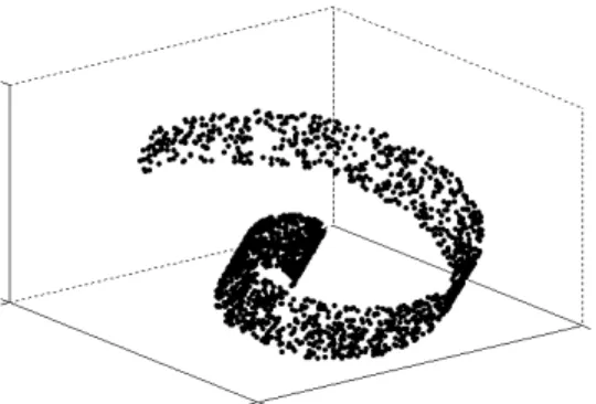
C.10 Multi-modal (XOR). . . 261
C.11 Redundant and one cluster per class . . . 261
D Graphs of artificial time series and human motion joint angle features 263 D.1 Artificial data sets . . . 263
D.2 Human motion data set . . . 266
D.2.1 Minimum, maximum and average features . . . 266
D.2.2 Window average and variance features . . . 272
List of Tables
2.1 Properties of common feature extraction techniques . . . 8
2.2 Feature set evaluation measures and their properties. . . 22
2.3 Comparison of multi-class extension methods. . . 43
3.1 FSHC accuracy estimation measures . . . 63
3.2 Description of FSHC artificial data set 1 . . . 63
3.3 Description of FSHC artificial data set 2 with noise . . . 64
3.4 Description of real data sets used for testing FSHC algorithm . . . 65
3.5 Results for FSHC artificial data set 1 with 0% and 5% noise . . . 68
3.6 Results for FSHC artificial data set 2 . . . 72
3.7 Accuracy FSCH and common multi-class extensions on different data sets . 73 3.8 Accuracy of FSHC across different runs while holding initialization or data set division constant . . . 76
3.9 Average and standard deviation of FSHC accuracies for ten runs using leave-one-out cross validation to estimate accuracy, using the same data set divi-sion and initialization parameters for all tests . . . 77
3.10 Number of features, base classifiers and memory footprint for FSHC and common multi-class extensions . . . 78
3.11 Training times for FSHC and common multi-class extensions . . . 80
3.12 Average number of classifiers, features and multiplications required to clas-sify a point using FSHC and common multi-class extensions . . . 82
3.13 Accuracy, number of features and number of base classifiers for data sets with added redundant and noisy features for FSHC and multi-class exten-sions with and without feature selection . . . 85
3.14 Properties of artificial and real data sets used for testing MBT and compar-ing filter-based feature set evaluation measures . . . 91
3.15 Accuracy of MBT and common multi-class extensions on artificial data sets 95
3.16 Accuracy of MBT and common multi-class extensions on real data sets . . 96
3.17 Number of base classifiers for MBT and common multi-class extensions ex-tensions using artificial data sets. . . 97
3.18 Number of base classifiers for MBT and common multi-class extensions using real data sets . . . 97
3.19 Total number of features used by MBT and common multi-class extensions for artificial data sets . . . 98
3.20 Total number of features used by MBT and common multi-class extensions for real data sets . . . 98
3.21 Average number of features required to classify each point using MBT and common multi-class extensions for artificial data sets . . . 99
3.22 Average number of features required to classify each point using MBT and common multi-class extensions for real data sets . . . 99
3.23 Comparison FS-MBT with differentrmc values on artificial data sets . . . . 100 3.24 Comparison FS-MBT with differentrmc values on real data sets . . . 101
4.1 Tested filter measures and parameters. . . 105
4.2 Properties of artificial data sets . . . 108
4.3 RELIEF-F correlations for different univariate combinations on artificial data sets . . . 110
4.4 RELIEF-F correlations for different univariate combinations on real data sets111
4.5 Ability of different measures to determine the informative features . . . 113
4.6 Correlation of filter values and 1-NN accuracies on artificial data sets . . . 114
4.8 Correlation of filter values and SVM one vs. one accuracies on artificial data
sets . . . 116
4.9 Correlation of filter values and SVM one vs. one accuracies on real data sets 117
4.10 Correlation of filter values and SVM one vs. all accuracies on artificial data
sets . . . 118
4.11 Correlation of filter values and SVM one vs. all accuracies on real data sets 119
4.12 Comparison of RELIEF-family correlation on artificial data sets . . . 121
4.13 Comparison of RELIEF-family correlation on real data sets . . . 122
4.14 Comparison of probability measure correlation on artificial data sets . . . . 124
4.15 Comparison of probability measure correlation on real data sets . . . 125
4.16 Correlation between filter values and 1-NN accuracy values for the Monk 2
data set with and without 1% added noise . . . 132
4.17 Variance of filter measure / KNN correlation on artificial data sets . . . 133
4.18 Variance of filter measure / KNN correlation on real data sets . . . 134
4.19 Variance of filter measure / SVM one vs. one correlation on artificial data
sets . . . 135
4.20 Variance of filter measure / SVM one vs. one correlation on real data sets. 136
4.21 Variance of filter measure / SVM one vs. all correlation on artificial data sets137
4.22 Variance of filter measure / SVM one vs. all correlation on real data sets . 138
4.23 Common data set challenges for feature selection . . . 146
4.24 Mutual information and conditional mutual information forMonk 1 data set 149
4.25 Ability of dCMIM and dFOU to find dependent and informative features . 154
4.26 Correlation of dCMIM and dFOU with classifier accuracy on artificial data sets, using best parameter set . . . 154
4.27 Correlation of dCMIM and dFOU with classifier accuracy on real data sets, using best parameter set . . . 155
5.1 Measured body features used in the real data sets in this work . . . 162
5.3 Binary problems with artificial data set . . . 163
5.4 SVM accuracy on kick vs. punch and throw vs. punch using CMIM . . . . 164
5.5 SVM accuracy on kick vs. punch and throw vs. punch using FOU . . . 165
5.6 Commonly selected features when selecting among minimum, maximum and average features . . . 166
5.7 Commonly selected features when selecting entire feature (not including minimum, maximum and average) . . . 167
5.8 Commonly selected features when selecting entire feature and the minimum, maximum and average are included as separate features in the set . . . 168
5.9 Commonly selected features when selecting individual time samples (not including minimum, maximum and average) . . . 169
5.10 Commonly selected features when selecting individual time samples and the minimum, maximum and average are included as separate features in the set 170 5.11 SVM accuracy on artificial data sets using two-stage feature selection . . . 172
5.12 Accuracy of MBT on three class human motion problem . . . 173
5.13 Accuracy of MBT on nine class human motion problem . . . 173
5.14 Hand gestures from first MYO armband data set . . . 180
5.15 Hand gestures from second MYO armband data set . . . 180
5.16 Features calculated from EMG data for hand gesture recognition . . . 181
5.17 Meta-features used for hand gesture recognition . . . 187
5.18 Confusion matrix for EMG 1 using a single stage MBT . . . 189
5.19 Precision and recall for each individual person on EMG 1 using a single stage MBT . . . 189
5.20 Confusion matrix for EMG 1 using a two-stage MBT . . . 189
5.21 Precision and recall for each individual person onEMG 1 using a two-stage MBT . . . 191
5.22 Accuracy of two-stage MBT on EMG 2 . . . 191
5.23 Commonly selected features for two-stage MBT onEMG 2 . . . 192
5.25 Accuracy of two-stage MBT classifier using cosine and full window features 194
5.26 Accuracy of MBT one vs. one classifier using cosine and full window features194
5.27 Average number of features used to classify a new point using a single stage
MBT classifier . . . 194
5.28 Average number of features used to classify a new point using a two-stage MBT classifier . . . 195
5.29 Average number of features used to classify a new point using a MBT one vs. one classifier . . . 195
A.1 Summary of 1-NN accuracy on different artificial data sets . . . 207
A.2 Summary of 1-NN accuracy on different real data sets . . . 207
A.3 Summary of SVM accuracy on different artificial data sets . . . 208
A.4 Summary of SVM accuracy on different real data sets . . . 209
B.1 RELIEF-F/classifier correlations on artificial data sets . . . 211
B.2 RELIEF-F/classifier correlations on real data sets . . . 212
B.3 subset RELIEF/classifier correlations on artificial data sets . . . 213
B.4 subset RELIEF/classifier correlations on real data sets . . . 214
B.5 KL/SVM correlations on artificial data sets . . . 215
B.6 KL/1-NN correlations on artificial data sets . . . 216
B.7 JS/SVM correlations on artificial data sets . . . 217
B.8 JS/1-NN correlations on artificial data sets . . . 218
B.9 Bhattacharyya/SVM correlations on artificial data sets . . . 219
B.10 Bhattacharyya/1-NN correlations on artificial data sets . . . 220
B.11 KL/SVM correlations on real data sets . . . 221
B.12 KL/1-NN correlations on real data sets . . . 222
B.13 JS/classifier correlations on real data sets . . . 223
B.14 Bhattacharyya/classifier correlations on real data sets . . . 224
B.16 SU/classifier correlations on artificial data sets . . . 226
B.17 MI/classifier correlations on real data sets . . . 227
B.18 SU/classifier correlations on real data sets . . . 228
B.19 mRMR/classifier correlations on artificial data sets . . . 229
B.20 CMIM/classifier correlations on artificial data sets . . . 230
B.21 FOU/classifier correlations on artificial data sets . . . 231
B.22 mRMR/classifier correlations on real data sets . . . 232
B.23 CMIM/classifier correlations on real data sets . . . 233
B.24 FOU/classifier correlations on real data sets . . . 234
B.25 Consistency/classifier correlations on artificial data sets . . . 235
B.26 Consistency/classifier correlations on real data sets . . . 236
B.27 LS/classifier correlations on artificial data sets (t parameter) . . . 237
B.28 LS/SVM correlations on artificial data sets (k parameter) . . . 238
B.29 LS/1-NN correlations on artificial data sets (k parameter) . . . 239
B.30 LS/classifier correlations on real data sets (t parameter) . . . 240
B.31 LS/SVM correlations on artificial data sets (k parameter) . . . 241
B.32 LS/1-NN correlations on artificial data sets (k parameter) . . . 242
B.33 MCFS/classifier correlations on artificial data sets (t parameter) . . . 243
B.34 MCFS/SVM one vs. one correlations on artificial data sets (k parameter) . 244 B.35 MCFS/SVM one vs. all correlations on artificial data sets (k parameter) . 245 B.36 MCFS/1-NN correlations on artificial data sets (k parameter) . . . 246
B.37 MCFS/classifier correlations on real data sets (t parameter) . . . 247
B.38 MCFS/SVM one vs. one correlations on real data sets (k parameter) . . . 248
B.39 MCFS/SVM one vs. all correlations on real data sets (k parameter) . . . . 249
B.40 MCFS/1-NN correlations on real data sets (k parameter) . . . 250
B.41 CFS/classifier correlations on artificial data sets . . . 251
List of Figures
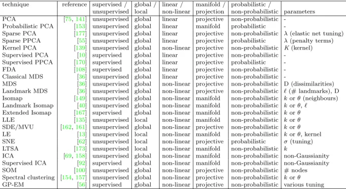
2.1 Swiss roll data set illustrating the concept behind manifold-based
dimen-sionality reduction techniques . . . 9
2.2 Data set illustrating the PCA procedure . . . 11
2.3 One vs. one extension for a three class problem . . . 39
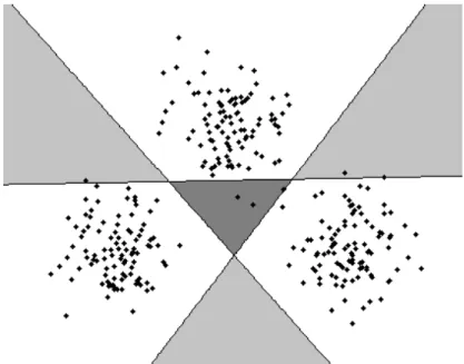
2.4 SVM and decision tree divisions of a linearly separable data set . . . 41
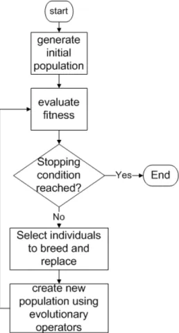
2.5 General flow of a genetic algorithm . . . 46
2.6 Common evolutionary operators . . . 47
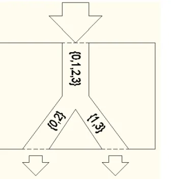
3.1 Dividing a multi-class problem into binary outputs . . . 55
3.2 Dividing a multi-class problem into multiple outputs . . . 56
3.3 Full genome used for feature selection and classifier construction . . . 57
3.4 Genes for two four-class hierarchical classifiers . . . 58
3.5 Pseudocode for calculating FSHC class separation layers . . . 59
3.6 Pseudocode for adding FSHC base classifiers . . . 59
3.7 Crossover functions . . . 62
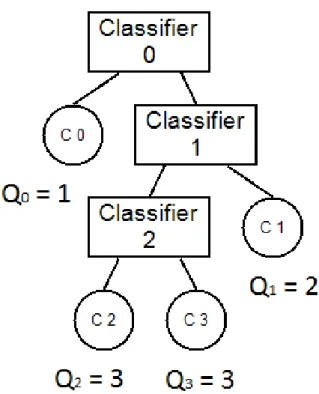
3.8 Example classification tree, with the number of queries required to classify each class . . . 68
3.9 Hierarchical classifiers generated for FSHC artificial data set 1 with no noise 69 3.10 Hierarchical classifiers generated for FSHC artificial data set 1 with 5% uniform random noise . . . 70
3.12 Dependent data sets . . . 90
3.13 Correlated data sets . . . 93
3.14 Two U’s data set . . . 94
4.1 1-NN accuracy on theMonk 2 data set for feature sets with different numbers of features . . . 130
4.2 1-NN accuracy on theMonk 2 data set with 1% uniform random noise added to each feature . . . 131
4.3 Selecting filter measures for use with KNN. Continued in Figure 4.4 . . . . 143
4.4 Selecting filter measures for use with KNN (continued). Continued from Figure 4.3. . . 144
4.5 Selecting filter measures for use with SVM . . . 145
4.6 Flow chart for using dCMIM or dFOU filter measure . . . 150
5.1 Classifier extensions for time-series data . . . 158
5.2 Tree-based classifier structure for three-class human motion classification problem . . . 174
5.3 Tree-based classifier structure for nine-class human motion classification problem . . . 175
5.4 RMS values for a single trial of the “snap” motion . . . 177
5.5 Top level of the two-stage tree designed using EMG 1 . . . 190
5.6 Top level of the two-stage tree designed using EMG 2 and four class problem192 D.1 Regular vs. low curve . . . 263
D.2 Regular vs. moved curve . . . 263
D.3 Regular vs. skinny curve . . . 264
D.4 Regular vs. stacked curve . . . 264
D.5 Regular vs. extra curve . . . 264
D.6 Regular vs. skinny curve with no added noise . . . 264
D.8 Minimum, maximum and average for right leg yaw . . . 266
D.9 Minimum, maximum and average for right leg roll . . . 266
D.10 Minimum, maximum and average for right leg pitch . . . 267
D.11 Minimum, maximum and average for right knee . . . 267
D.12 Minimum, maximum and average for right ankle pitch . . . 267
D.13 Minimum, maximum and average for right ankle yaw . . . 267
D.14 Minimum, maximum and average for right shoulder pitch . . . 268
D.15 Minimum, maximum and average for right shoulder yaw . . . 268
D.16 Minimum, maximum and average for right elbow roll . . . 268
D.17 Minimum, maximum and average for right elbow pitch . . . 268
D.18 Minimum, maximum and average for left leg yaw . . . 269
D.19 Minimum, maximum and average for left leg roll . . . 269
D.20 Minimum, maximum and average for left leg pitch . . . 269
D.21 Minimum, maximum and average for left knee . . . 269
D.22 Minimum, maximum and average for left ankle pitch . . . 270
D.23 Minimum, maximum and average for left ankle roll . . . 270
D.24 Minimum, maximum and average for left shoulder pitch . . . 270
D.25 Minimum, maximum and average for left shoulder pitch . . . 270
D.26 Minimum, maximum and average for left elbow roll . . . 271
D.27 Minimum, maximum and average for left elbow pitch . . . 271
D.28 Window average and variance features for right leg yaw . . . 272
D.29 Window average and variance features for right leg roll . . . 272
D.30 Window average and variance features for right leg pitch . . . 273
D.31 Window average and variance features for right knee . . . 273
D.32 Window average and variance features for right ankle pitch . . . 274
D.33 Window average and variance features for right ankle roll . . . 274
D.35 Window average and variance features for right shoulder yaw . . . 275
D.36 Window average and variance features for right elbow roll . . . 276
D.37 Window average and variance features for right elbow pitch . . . 276
D.38 Window average and variance features for left leg yaw . . . 277
D.39 Window average and variance features for left leg roll . . . 277
D.40 Window average and variance features for left leg pitch . . . 278
D.41 Window average and variance features for left knee . . . 278
D.42 Window average and variance features for left ankle pitch . . . 279
D.43 Window average and variance features for left ankle roll . . . 279
D.44 Window average and variance features for left shoulder pitch . . . 280
D.45 Window average and variance features for left shoulder yaw . . . 280
D.46 Window average and variance features for left elbow roll . . . 281
Acronyms
1-NN 1-nearest neighbour.
ABT Adaptive binary tree.
ACO Ant colony optimization.
ANN Artificial Neural Network.
AR Auto-regressive.
BDT Binary decision tree.
CART Classification and regression tree.
CFS Correlation feature selection.
CMI Conditional mutual information.
CMIM Conditional mutual information maximization.
CPFS Convex principal feature selection.
CV Cross validation.
DAG-SVM Directed acyclic graph support vector machine.
dCMIM Dependency aware conditional mutual information maximization.
dFOU Dependency aware fist order utility.
DWT Discrete wavelet transform.
EMG Electromyography.
FDA Fisher’s discriminant analysis.
FIS Fuzzy inference system.
FOU First order utility.
GA Genetic algorithm.
GPLVM Gaussian process latent variable model.
GSBS Generalized sequential backwards search.
GSFS Generalized sequential forward search.
HMM Hidden Markov model.
ICA Independent component analysis.
IFFS Improved forward floating search.
JS Jensen-Shannon.
KL Kullback-Leibler.
KNN / K-NN K-Nearest neighbours.
KPCA Kernel principal component analysis.
LASSO Least-absolute selection and shrinkage operator.
LDA Linear discriminant analysis.
LE Laplacian eigenmaps.
LLE Locally linear embedding.
LOSO / LOSO-CV Leave-one-subject-out cross validation.
LS Laplacian score.
LTSA Local tangent space alignment.
LVF Las Vegas Filter.
MAV Mean absolute value.
MBT Multi-modal binary tree.
MCFS Multi-cluster feature selection.
MDS Multi-dimensional scaling.
MI Mutual information.
MLP Multi-layer perceptron.
mRMR minimal-redundancy maximal-relevancy.
MVU Maximum variance unfolding.
OS Oscillating search.
OVO One vs. one.
OVR One vs. rest.
PCA Principal component analysis.
PPCA Probabilistic principal component analysis.
PSO Particle swarm optimization.
PTA Plus-l-minus-r.
RBF Radial basis function network.
RMS Root mean squared.
SBFS Sequential backwards floating search.
SBS Sequential backwards search.
SDE Semi-definite embedding.
SFFS Sequential forward floating search.
SFS Sequential forward search.
SNE Stochastic neighbour embedding.
SOM Self-organizing map.
SPCA Sparse principal component analysis / Supervised principal component analysis.
SS-GPLVM Simple sequence Gaussian process latent variable model.
SSI Simple squared integral.
ST-Isomap Spatio-temporal Isomap.
SU Symmetric uncertainty.
SVM Support Vector Machine.
Glossary
K-folds cross validation K-folds cross validation is a method of estimating classifier
accuracy. The data set is divided into K approximately equal sized groups or folds.
K classifiers are trained, each leaving one fold out of the training set and assessing
the trained classifier on the removed points. K-folds cross validation can be used as
a wrapper-based feature subset evaluation measure.
1-nearest neighbour The 1-nearest neighbour is a form of the K-nearest neighbours
classification algorithm that uses only a single neighbour.
Adaptive binary tree (ABT) The adaptive binary tree is a type of hierarchical classi-fier based on a one vs. one training [27].
Additive multivariate Additive multivariate feature selection measures consider the benefit of each unselected feature with respect to the selected set. These are dif-ferent than univariate measure because they consider the value of each feature with respect to the selected features rather than in isolation. Additive multivariate mea-sures are different than grouped multivariate meamea-sures, which consider the benefit of a group of features as a whole rather than the additional benefit gained by adding a new feature.
Ant colony optimization (ACO) Ant colony optimization is a type of stochastic opti-mization technique that can be used for feature selection.
Artificial neural network (ANN) An artificial neural network is an algorithm used for classification or regression.
Auto-regressive coefficients (AR coefficients) An autoregressive model of a
time-series signal models the current sample as a weighted sum of past samples in the time-series. The AR coefficients are the weights used for the past samples.
Autoencoder An autoencoder is a type of artificial neural network where the output values are designed to match the input values. Autoencoders can be used for feature extraction by using the hidden node values as features.
Bhattacharyya divergence Bhattacharyya divergence is a divergence measure used to
assess the difference between probability distributions. Bhattacharyya divergence can be used as a univariate feature selection measure, where it is used to measure the difference between the distributions of different classes [14].
Binary classifier A binary classifier is a classifier that is only capable of distinguishing between two classes of inputs.
Binary decision tree (BDT) The binary decision tree is a type of hierarchical classifier based on a technique similar to k-means clustering [103].
Classification and regression tree (CART) The classification and regression tree is a decision tree algorithm that can be used for classification or regression.
Classifier Classifiers are algorithms that determine the label or class of a sample based on its characteristic features.
Clustering Clustering techniques aim to divide points into groups or clusters based on their characteristic features. Clustering techniques are unsupervised and hence do not use class labels to help determine the grouping.
Conditional mutual information Conditional mutual information measures the
mu-tual information between two variables given a third variable. The notation for
con-ditional mutual information is I(A;B|C), which indicates the mutual information
between A and B given C.
Conditional mutual information maximization (CMIM) Conditional mutual
infor-mation maximization is an additive multivariate feature subset evaluation measure based on the conditional mutual information between a feature and the class given the selected features [48].
Consistency Consistency is a grouped multivariate feature subset evaluation measure that is based on the number of inconsistent points in a set. Two samples are con-sidered to be inconsistent if they have the same input feature values, but a different class label [37].
Convex principal feature selection (CPFS) Convex principal feature selection is an algorithm for feature selection that treats feature selection as a direct optimization problem [109].
Correlated features A correlated feature is any feature whose value can be predicted to some extent from other features.
Correlation feature selection (CFS) Correlation feature selection is a grouped multi-variate feature subset evaluation measure where the goal is to maximize the mutual information between the selected features and the class and minimize the mutual information between the selected features [58].
Dependency aware conditional mutual information (dCMIM) Dependency aware
conditional mutual information is a feature subset evaluation measure proposed in this thesis. The dCMIM is based on the CMIM feature measure, but includes an extra step that explicitly looks for dependent features in the set.
Dependency aware first order utility (dFOU) Dependency aware first order utility
is a feature subset evaluation measure proposed in this thesis. The dFOU is based on the FOU and CFS feature measures, but includes an extra step that explicitly looks for dependent features in the set.
Dependent features A data set with dependent features includes one or more features that work together to separate the data set, but cannot separate the data set on their own.
Directed acyclic graph support vector machine (DAG-SVM) Directed acyclic graph
support vector machine is a multi-class extension for support vector machines that is based on a one vs. one training. A classifier is trained on each pair of classes and these pairwise classifiers are used to successively eliminate classes from consideration. This means that the time required to classify new points is shorter than the one vs. one multi-class extension on which it is based, because fewer classifiers need to be queried. DAG-SVM was proposed in [126].
Discrete wavelet transform (DWT) The discrete wavelet transform is the type of
wavelet decomposition used for discrete signals. The discrete wavelet transform di-vides the signal by passing it through a high and a low pass filters, downsamples each side and successively applies the high and low pass filters to the low frequencies.
Dynamic oscillating search (DOS) Dynamic oscillating search is a type of sequential feature subset selection technique used in feature selection problems. DOS is an extension of OS and unlike its forwards and backwards counterparts, SFFS and SBFS, DOS begins with a set of pre-selected features [144].
Electromyography (EMG) Electromyography uses sensors to detect muscle activation.
Envelope The envelope of a signal gives the general signal shape. It is a low pass filtered version of the rectified signal.
Feature A feature is the input to a classifier. Features describe some aspect of the data and can be quite simple (ex. raw data) or extremely complex (ex. values calculated from raw data).
Feature extraction Feature extraction techniques are used to transform a given set of input features to create a new set of features that have some desired property.
Feature measure Please see “feature subset evaluation measure”.
Feature Selected Hierarchical Classifier (FSHC) The feature selected hierarchical
classifier is a hierarchical classifier proposed in this thesis that uses a genetic algorithm to jointly perform feature selection and to design the class separation that defines the classifier structure.
Feature selection Feature selection is used to select a subset of good features from a larger set of candidate features. The selected subset forms the set of classifier inputs. Feature set selection technique The feature set selection technique is a component of feature selection algorithms. The feature set selection technique guides the feature subset search based on the information provided by the feature subset evaluation measure.
Feature subset evaluation measure The feature subset evaluation measure is a
com-ponent of feature selection algorithms. The feature subset evaluation measure is used to estimate the “goodness” of a particular set of features.
Filter A filter is a type of feature subset evaluation measure, where the feature subset is evaluated using a calculated value instead of direct testing on the desired classifier.
First order utility (FOU) First order utility is an additive multivariate feature subset evaluation measure that combines the conditional mutual information terms used in CMIM and feature-feature mutual information terms used in mRMR [20].
Fisher’s discriminant analysis (FDA) Fisher’s discriminant analysis is a supervised linear feature extraction technique. It is closely related to linear discriminant analysis (LDA) and the terms are sometimes used interchangeably, though FDA most com-monly refers to the feature extraction technique while LDA most comcom-monly refers to the classification technique.
Fisher’s interclass separability criterion Fisher’s interclass separability criterion is a grouped multivariate feature subset evaluation measure that evaluates feature subsets based on the ratio of within-class to between-class distances [43].
Fuzzy inference system (FIS) A fuzzy inference system is a type of classifier of regres-sion system based on fuzzy logic.
Gaussian process latent variable model (GPLVM) Gaussian process latent variable
models can be used as an unsupervised, non-linear feature extraction technique [94].
Generalized sequential backwards search (GSBS) Generalized sequential backwards
search is a type of sequential feature subset selection technique used in feature se-lection problems. It is an extension of SBS. GSBS is less commonly used than its floating counterpart SFBS, becasue GSBS requires parameter settings [80].
Generalized sequential forwards search (GSFS) Generalized sequential forwards search
is a type of sequential feature subset selection technique used in feature selection problems. It is an extension of SFS. GSFS is less commonly used than its floating counterpart SFFS, becasue GSFS requires parameter settings [80].
Genetic algorithm (GA) Genetic algorithms are a type of stochastic optimization tech-nique that can be used for feature selection.
Graph Laplacian The graph Laplacian is a representation of the similarity graph where the matrix entries are based on the difference between the similarity graph and the diagonal graph representing all the weight connections to each point.
Grouped multivariate Grouped multivariate feature selection measures consider the
benefit of a feature subset as a whole. Grouped multivariate measures are different than additive multivariate measures, which consider the additional benefit gained by adding a new feature rather than the benefit of the entire group.
Hidden Markov model (HMM) A hidden Markov model is a method for modeling time series data. HMMs can be used for classification by training one model per class.
Hierarchical classifier A hierarchical classifier is a multi-class extension where the set of classes is progressively divided into smaller subsets until there is only one class remaining at each node. See also Tree-based classifier.
Hjorth parameters The Hjorth parameters are EMG-specific features. There are three Hjorth parameters: activity, mobility and complexity. The parameters measure the ratio of variances for the signal and its derivatives [64].
Improved forward floating search (IFFS) Improved forward floating search is a type of sequential feature subset selection technique used in feature selection problems. It is an extension of SFFS [116].
Independent component analysis (ICA) Independent component analysis is a method
of blind signal separation that can be used as an unsupervised feature extraction technique [33].
Isomap Isomap is an unsupervised, non-linear, neighbourhood based feature extraction technique [149].
Jensen-Shannon divergence (JS) Jensen-Shannon is a divergence measure used to
as-sess the difference between probability distributions. JS can be used as a univariate feature selection measure, where JS is used to measure the difference between the distributions of different classes [97].
K-means clustering K-means clustering is a clustering technique that separates points into K clusters with the smallest grouped distance to the class center.
K-nearest neighbours K-nearest neighbours is a classification algorithm where the class of a point is determined by a vote of the K closest points in the training set [34].
Kernel principal component analysis (KPCA) Kernel principal component analysis
is an unsupervised, non-linear feature extraction technique based on PCA [141].
Kullback-Leibler divergence (KL) Kullback-Leibler is a divergence measure used to
assess the difference between probability distributions. KL can be used as a univariate feature selection measure, where KL is used to measure the difference between the distributions of different classes [90].
Kurtosis The kurtosis of a signal measures its peakedness.
Laplacian eigenmap (LE) Laplacian eigenmap is an unsupervised, non-linear,
neigh-bourhood based feature extraction technique [13].
Laplacian score (LS) Laplacian score is an unsupervised, neighbourhood based feature subset evaluation measure [61].
Las Vegas filter (LVF) Las Vegas filter is randomized search technique that can be used for feature selection.
Least absolute selection and shrinkage operator (LASSO) The least absolute
se-lection and shrinkage operator can be used to perform embedded feature sese-lection. LASSO adds the minimization of a 1-norm operator to a standard regression or clas-sification optimization problem. The inclusion of this additional term encourages the weights for some inputs to become zero. This sparsity in the weights is a form of embedded feature selection [150].
Leave-one-out cross validation (LOOCV) Leave-one-out cross validation is a method
of estimating classifier accuracy. N classifiers are trained,whereN is the number of
data points. Each classifier leaves one point out from the training set and evaluates
the classifier on the untrained point. LOOCV is also called N-folds cross validation.
LOOCV can be used as a wrapper-based feature subset evaluation measure.
Leave-one-subject-out cross validation (LOSO) Leave-one-subject-out cross
valida-tion is a method of estimating classifier accuracy when the data set contains data
from more than one subject. S classifiers are trained,where S is the number of
sub-jects. Each classifier leaves the data from one subject out from the training set and evaluates the classifier on the data from the untrained subject.
Linear discriminant analysis (LDA) Linear discriminant analysis is a binary, linear classification technique. It is closely related to Fisher’s discriminant analysis (FDA) and the terms are sometimes used interchangeably, though FDA most commonly refers to the feature extraction technique while LDA most commonly refers to the classification technique.
Local tangent space alignment (LTSA) Local tangent space alignment is an
unsu-pervised, non-linear, neighbourhood-based feature extraction technique [173].
Locally linear embedding (LLE) Locally linear embedding is an unsupervised,
Maximum variance unfolding (MVU) Maximum variance unfolding is an unsuper-vised, non-linear, neighbourhood based feature extraction method [161].
Mean absolute value (MAV) The mean absolute value is measured over a finite
por-tion of a time-series signal. The absolute value of each sample is taken, then these values are averaged.
Minimal-redundancy maximal-relevancy (mRMR) Minimal-redundancy
maximal-relevancy is an additive multivariate feature subset evaluation measure based on the mutual information between the feature and the class and between the feature and other features in the selected set [122].
Monotonic A monotonic data set is a data set where the classification accuracy will never decrease when a new feature is added to the selected set.
Motion recognition Motion recognition is a type of classification problem where the challenge is to recognize the movement being performed from a set of known move-ments.
Multi-class classifier A multi-class classifier is a classifier that is capable of distinguish-ing between more than two classes of inputs.
Multi-class extension A multi-class extension is a method for dividing multi-class classi-fication problems into sets of binary problems, normally for use with binary classifiers.
Multi-cluster feature selection (MCFS) Multi-cluster feature selection is an unsu-pervised, neighbourhood-graph-based feature subset evaluation measure [23].
Multi-dimensional scaling (MDS) Multi-dimensional scaling is an unsupervised
fea-ture extraction technique [18].
Multi-layer perceptron (MLP) A multi-layer perceptron is a type of artificial neural network.
Multi-modal Binary Tree (MBT) The multi-modal binary tree is a hierarchical
clas-sifier proposed in this thesis that tolerates misclassification of the training samples by adding additional classifiers to re-classify initially misclassified points. This creates a linear piecewise separation of the data.
Multivariate Multivariate indicates that multiple variables are being considered together. Multivariate feature selection measures consider subsets of features as a group.
Mutual information (MI) Mutual information is a measure of the dependence between
a pair of variables. Mutual information can be used as a univariate feature set
evaluation measure by measuring the mutual information between the feature and the class label [102].
Naive Bayes Naive bayes is a type of classifier that is based on Bayesian probability.
Neighbourhood graph The neighbourhood graph is a type of similarity graph where
neighbouring points are connected by some weight, but non-neighbouring points are unconnected (zero weight).
Non-monotonic A non-monotonic data set is a data set that contains at least one feature that is not monotonic. In this case, adding a feature to the selected set will decrease classification accuracy.
One vs. one One vs. one is a multi-class extension that trains a classifier for each pair of classes. The overall classification of a point is determined by vote.
One vs. rest One vs. rest is a multi-class extension that requires training one classifier per class. Each classifier classifies between points from a single class and points in the remaining classes.
Oscillating search (OS) Oscillating search is a type of sequential feature subset selection technique used in feature selection problems. Unlike its forwards and backwards counterparts, SFFS and SBFS, OS begins with a set of pre-selected features [145].
Particle swarm optimization (PSO) Particle swarm optimization is a type of stochas-tic optimization technique that can be used for feature selection.
Plus-l-minus-r (PTA) Plus-l-minus-r is a type of sequential feature subset selection technique used in feature selection problems. It is an extension of SFS. PTA is less commonly used than its floating counterparts SFFS because PTA requires parameter settings [146].
Principal component analysis (PCA) Principal component analysis is an
unsuper-vised, linear feature extraction technique [75].
Probabilistic principal component analysis (PPCA) Probabilistic principal
compo-nent analysis is an unsupervised, linear feature extraction technique based on PCA [153].
Pure noise feature A pure noise feature is a feature that contains no information about the class label. See also “Random feature”.
Radial basis function network (RBF) A radial basis function network is a type of
artificial neural network.
Random feature A random feature is a feature that contains no information about the class label. See also “Pure noise feature”.
Redundant features A redundant feature is a feature that is an exact copy of another feature in the set.
RELIEF / RELIEF-F RELIEF-F is a univariate feature subset evaluation measure that
assesses the value of a feature or feature subset (subset-RELIEF) based on the
dis-tance to neighbouring points in the same and different classes [79, 82].
Root mean squared (RMS) The root mean squared value is measured over a finite
portion of a time-series signal. Each of the values is squared, the squared values are then averaged and the square root of the average of the squared values is taken.
Self-organizing map (SOM) Self-organizing map is a clustering technique that is com-monly used for data visualization.
Semi-definite embedding (SDE) Semi-definite embedding is a method for performing
maximum variance unfolding (MVU) feature extraction [162].
Sequential backwards floating search (SBFS) Sequential backwards floating search
is a sequential feature subset selection technique used in feature selection problems. SBFS is based on SBS, but allows features to be re-added at each step [127].
Sequential backwards search (SBS) Sequential backwards search is a sequential fea-ture subset selection technique used in feafea-ture selection problems where feafea-tures are removed one at a time from a full set [107].
Sequential forwards floating search (SFFS) Sequential forwards floating search is a sequential feature subset selection technique used in feature selection problems. SFFS is based on SFS, but allows features to be removed at each step [127].
Sequential forwards search (SFS) Sequential forwards search is a sequential feature subset selection technique used in feature selection problems where features are added one at at time to the selected set [165].
Similarity graph A similarity graph is a way of representing data in graph form. Each input point represents one node in the graph and the weights between each point describes how similar the points are.
Similarity matrix A similarity matrix is a representation of the similarity graph in
ma-trix form. The mama-trix entry at ij represents the weight (similarity) between nodes i
and j in the similarity graph..
Simple sequence Gaussian process latent variable model (SS-GPLVM) The
SS-GPLVM is a type of SS-GPLVM that can be used for motion recognition [16].
Simple squared integral (SSI) The simple square integral is measured over a finite portion of a time-series signal. Each sample is squared and summed to give the SSI.
Simulated annealing (SA) Simulated annealing is a type of stochastic optimization
technique that can be used for feature selection.
Skewness The skewness of a signal measures its asymmetry.
Sparse Principal component analysis (Sparse PCA / SPCA) Sparse principal
com-ponent analysis is an unsupervised, sparse, linear feature extraction technique based on PCA [177].
Spatio-temporal Isomap (ST-Isomap) ST-Isomap is a version of the Isomap feature
extraction technique that can be used with temporal data [72].
Spectral clustering Spectral clustering is a clustering technique that is based on the similarity graph [157].
Stochastic neighbour embedding (SNE) Stochastic neighbour embedding is an
un-supervised, non-linear, neighbourhood based feature extraction technique [62]. Supervised Supervised techniques use the class labels as well as the input features as a
part of an algorithm.
Support vector machine (SVM) A support vector machine is a binary classifier that
separates points in different classes using a hyperplane whose location is determined by the largest margin between the classes.
Symmetric uncertainty (SU) Symmetric uncertainty is a univariate mutual-information-based feature subset evaluation measure [169].
Tabu search Tabu search is a type of stochastic optimization technique that can be used for feature selection.
Tree-based classifier A tree-based classifier is a multi-class extension where the set of classes is progressively divided into smaller subsets until there is only one class re-maining at each node. See also Hierarchical classifier.
UCI machine learning repository The UCI machine learning repository is a collection of data sets maintained by the University of California, Irvine [8].
Univariate Univariate indicates that only one variable is being considered. Univariate feature selection measures consider each feature in isolation.
Unsupervised Unsupervised techniques do not use the class labels as a part of the algo-rithm, and base the algorithm output only on the properties of the input features.
Validation set A validation set is a portion of the data set that is withheld from the training set when training a classifier or a regression algorithm. This portion of the data set is then used for testing in order to test the generalization ability of the algorithm.
Wavelet The wavelet decomposition of a signal is similar to short time Fourier analysis, but instead of using equally sized windows for each frequency component, wavelets match the size of the window to the frequency being analyzed. Rather than the sine wave decomposition used in Fourier analysis, wavelet decomposition performs a successive convolution of the signal with scaled and shifted versions of a finite length mother wavelet.
Willson Amplitude The Willson amplitude is measured over a finite portion of a time-series signal. The Willson amplitude counts the number of times the signal value change between samples is larger than a pre-determined threshold.
Wrapper A wrapper is a type of feature subset evaluation measure where the performance of the feature subset is evaluated directly on the classifier.
Zero crossings (ZC) The number of zero crossings is measured over a finite portion of a time-series signal. The ZC measures the number of time the signal value changes signs.
Chapter 1
Introduction
Classification algorithms estimate the class of a sample based on its characteristic features. Classifiers are used in many different domains for tasks ranging from simple taxonomy to complex medical classification and computer vision applications.
The performance of a classifier is affected by a number of different factors including classifier type and parameters, the input features and the desired outputs. This thesis examines the selection of input features and how the selected features and output groupings jointly contribute to the overall performance of the classifier.
Feature selection is an important and difficult problem in machine learning. Good feature selection can improve classifier performance in a number of ways. Selecting a good subset of features not only decreases the computational load, but can also improve accuracy [50]. Feature selection lessens the impact of noisy features, which can cause false association between relatively random features and the classifier output. Feature selection can also help to identify redundant or correlated features, which increase classifier complexity without adding much additional information [57]. In some cases, the features may be informative for differentiating between some classes, but not others. Including these partially informative features may also degrade performance. Feature sets may also contain dependent features, which are not useful by themselves but provide significant information when combined with other features [57].
Feature selection is complicated by the fact that multi-way dependencies and corre-lations can exist, meaning simply selecting the best individually scored features may not produce the best set. Hence good feature selection requires not just individual or pairwise feature evaluation, but evaluations of entire subsets [57]. Additionally, because of feature
dependence, the optimal set of N features may not include the optimal set of N −1 fea-tures [127]. This greatly increases the number of evaluations required to properly evaluate a feature set.
Different classifiers tend to have different tolerances for feature sets with redundant and correlated features [57]. This also means that the feature set evaluation criterion needs to be classifier-specific to properly capture the utility of the feature set being investigated.
The most obvious way to tailor a feature set to a specific classifier is to evaluate the feature set directly on the desired classifier. This type of feature evaluation is called a “wrapper” method. While wrappers tend to perform well, since they give direct feedback about the ability of the classifier to use the feature set [81], they are computationally expensive. They can also select features that are too specific to the training set, causing generalization problem. This is a particular problem if the number of samples is small [143].
Filter measures do not evaluate the feature set directly on the classifier, but instead use a calculated value as an estimate of the feature set performance. Filter measures tend to be less computationally expensive than wrappers, but do not directly measure the ability of the selected classifier to use the feature set. The ideal measure of a feature set would be a filter measure that is known to be a good estimate of accuracy for a particular classifier. This measure would likely be different for different classifiers.
The decision about which outputs to use can also significantly affect the classification accuracy. Trying to classify a set with a small number of classes will often be easier than trying to differentiate between larger numbers of possibilities. It is also often easier to classify points when the classes are very different from each other than it is to make fine distinctions between similar categories. Unfortunately, the output classes are most often set a-priori and cannot be changed.
The standard approach to multi-class classification is to use a single classifier with many outputs. However, another option is to split the problem into a set of classification problems that each use only a subset of the classes or samples. Dividing the problem is always necessary when binary classifiers are used to classify multi-class problems. Splitting the problem can increase the overall accuracy multi-class classifiers [137]. Problem division allows the use of a more specific set of features for each set of classes. For some classifiers, better generalization can be achieved by sparse set of inputs [106]. Splitting a multi-class problem also affects the input feature selection process since some features may be more informative about certain class subsets.
The question of how to divide the problem is not trivial and remains an active research area. There are a number of common methods for dividing a multi-class problem for use
with binary classifiers. These include one vs. rest, where a classifier is trained for each class to classify it from the others, and one vs. one, where classifiers are trained on each pair of classes and a voting scheme is used. Unfortunately, it does not appear that any one
method is the best solution in all cases [132, 65]. Tree-based classifiers divide the problem
hierarchically, with each level splitting the classification task into a progressively smaller
set of classes [29, 103]. Trees are intuitively a good choice because they do not require all
the trained classifiers to be queried to perform a classification, reducing classification time. There are three major components to this thesis, each exploring a different aspect of feature selection and output division. The first part of this thesis examines the joint contribution of feature selection and problem division on classification accuracy and com-putational complexity when using tree-based classifiers. Two different feature-selected tree-based classifiers are proposed and compared to other common multi-class extensions. The first proposed method uses genetic algorithms to jointly optimize the tree design and selected features. The second method performs the class division and feature selection sequentially. It also allows classes to appear at more than one leaf node. This allows it to classify multi-modal or non-linearly separable classes using piecewise classification.
The second part of the thesis examines the feature selection measure problem more closely. There have been a large number of feature evaluation measures proposed in the literature. For a researcher looking to use feature selection as a tool for solving a specific problem, the large number of potential solutions and the lack of direct comparison currently available in the literature can make it difficult to determine which measures are most suitable for a particular application or classifier. Testing a large number of filter measures is impractical in many cases, especially when the feature selection method is not the only parameter to be tuned. The second part of this thesis examines a number of well-known filter measures and compares their performance based on their ability to select informative features and correlation with classifier accuracy. Several different promising filter-based measures are recommended and two new measures are proposed that overcome some of the shortcomings of the tested methods.
The final part of the thesis examines feature selection for time-series data. Adding time-delay inputs to a classifier is essentially the same as adding new features, and their contribution to the overall accuracy and speed needs to be jointly considered when selecting features. The final part of the thesis examines whether feature selection techniques can be used to select individual time windows from within a time series as a way to improve classifier accuracy or reduce classification time. It then applies the selected feature selection measure and tree-based classifier to two time-series human motion recognition problems.
clas-sification problems that have noisy, correlated or irrelevant features. The classifier is par-ticularly beneficial for multi-modal or non-linearly separable problems where the training can be performed offline, but the classification of new points must be fast in order to clas-sify incoming data points in an online manner. Human motion recognition is selected as an exemplar multi-class time-series class problem. The human motion recognition prob-lems in this thesis have non-linearly separable classes and have many noisy, correlated and irrelevant features. Motion recognition was therefore considered to be an interesting and challenging domain in which to test the proposed algorithm.
This thesis makes the following contributions
• The development of a feature-selected tree-based classifier that can be used to classify
multi-modal and non-linear classes using piecewise separation
• An extensive empirical evaluation of current filter-based feature set evaluation
mea-sures with respect to specific classifiers
• The development of a new filter-based feature selection measure that can account for
dependent features
• The application of feature selection and the MBT algorithm to two different
time-series human motion recognition problems
The remainder of this thesis is organized as follows. Chapter 2 reviews the current
literature on feature selection and multi-class extensions including tree-based hierarchical classifiers. It also provides background on the techniques employed in this thesis. Chapter
3presents and evaluates two feature-selected tree-based classification algorithms. Chapter
4presents an empirical evaluation of common filter-based feature selection techniques and
proposes two new filter-based measures that explicitly look for dependent features. Chapter
5 presents an evaluation of feature selection techniques for time-series data and applies
feature selection and the proposed hierarchical classifier to two time-series human motion
recognition problems. Chapter 6 presents the conclusions and proposes future directions
Chapter 2
Previous Work
This chapter overviews the current work on feature extraction and selection and multi-class extensions for binary multi-classifiers including hierarchical multi-classifiers. It also provides background on the techniques employed in this thesis, including genetic algorithms, K-nearest neighbours classification (KNN), support vector machines (SVM) and K-means clustering.
2.1
Notation
A classification problem has a set of inputs X ∈ RF and a set of class labels Y. X is an
F ×N matrix, where N is the number of samples and F is the number of variables or
“features” in each sample. Yis anN dimensional vector of class labels, where the number
of classes is C. Each feature can either be continuous, where it can take any value in its
range, or discrete, where it can take only a certain set of values. Continuous features can
be discretized by placing the continuous samples into a set number of bins Nb.
Supervised techniques use both the inputs X and the class labels Y. Unsupervised
measures use only the inputs X.
2.2
Feature Selection and Feature extraction
Feature selection and feature extraction are often used as pre-processing steps for pat-tern recognition to improve accuracy and reduce computational complexity. While feature
extraction techniques are often formulated as optimization problems, feature selection tech-niques are typically formulated as search problems.
Feature extraction applies a transform to the given set of measurements to create a set of derived features:
Z=f(X) (2.1)
For linear feature extraction techniques, this can be formulated as a matrix transfor-mation.
Z=BX (2.2)
whereB is the Q×F transformation matrix.
Dimensionality reduction is achieved as part of the transformation, by setting Q < F.
Alternately, B can be an F ×F matrix, and a feature selection technique can be used to
select from the transformed features.
Feature selection aims to find a Q-dimensional subset of features, SQ, (Q ≤ F) that
optimizes classifier performance and optionally minimizes the feature set size.
Feature selection and extraction problems are closely related; feature selection can be
viewed as a restricted form of linear feature extraction (Equation 2.2), where the matrix
B is restricted to be a diagonal binary matrix. However, feature selection is more often
formulated as a search problem, where the goal is to find the best subset of features, based on some measure of feature set fitness.
Feature selection techniques are sometimes preferred over feature extraction techniques because they return a set of features that have real-world meaning. This can provide insight into which parts of the system are important. Additionally, feature selection can reduce the cost associated with acquiring features. While some pattern recognition tasks use features that have little associated cost (for example, the individual pixel values in an image), it is also possible to have features that have an associated computational or monetary cost (for example, frequency domain features that have a computational cost or medical tests that have a monetary cost). When features have an associated cost of any type, it can be beneficial to use feature selection to reduce the number of features that initially have to be generated. On the other hand, feature extraction can be used to generate features that are not in the original set, which can be more powerful.
Although feature extraction and feature selection are often presented as being two different, competing methods for dimensionality reduction, they can also be complimentary. Feature extraction techniques can be viewed as a feature generation stage that expands the number of available features, and feature selection can be viewed as the dimensionality
reduction stage that reduces the size of the feature set [44]. Depending on the data set and the classifier, the original feature set may be better for classification [162]. Hence, including the original feature set along with the transformed features may improve accuracy, if the feature selection technique is able to properly account for correlations in the features.
There are a large number of both feature extraction and feature selection techniques. These techniques are discussed and compared in the following sections.
2.3
Feature extraction techniques
Although feature extraction techniques are not the focus of this thesis, feature extrac-tion and feature selecextrac-tion can be used together and share many goals. Ideas and tech-niques from the field of feature extraction have been incorporated into feature selection algorithms and the fields are closely related. For example, Fisher’s discriminant analysis feature extraction is closely related to Fisher’s interclass separability criterion in feature selection. Neighbourhood-graph based feature selection techniques such as Laplacian score were mo