Analytical Solution of Time Dependent Diffusion Equation in Stable Case

http://www.sciencepublishinggroup.com/j/ajese doi: 10.11648/j.ajese.20180202.12

ISSN: 2578-7985 (Print); ISSN: 2578-7993 (Online)

Analytical Solution of Time Dependent Diffusion Equation

in Stable Case

Khaled Sadek Mohamed Essa, Sawsan Ibrahim Mohamed El Saied, Ayman Marrouf

Department of Mathematics and Theoretical Physics, NRC, Atomic Energy Authority, Cairo, Egypt

Email address:

To cite this article:

Khaled Sadek Mohamed Essa, Sawsan Ibrahim Mohamed El Saied, Ayman Marrouf. Analytical Solution of Time Dependent Diffusion Equation in Stable Case. American Journal of Environmental Science and Engineering. Vol. 2, No. 2, 2018, pp. 32-36.

doi: 10.11648/j.ajese.20180202.12

Received: May 27, 2018; Accepted: June 8, 2018; Published: August 9, 2018

Abstract:

The normalized integrated concentration of pollutant has been obtained after solving temporaly diffusion equation using the method of separation variable considering the eddy diffusivities which measuring at night or at any time in high inversion layer in the stable condition. The dataset is observed from the “Project prairie Grass” (Barad 1958) which is measured using wind speed at 1.5m and downwind distance during the experiment at 50, 200 and 800 m in stable case for runs from 1 to 10. Comparison between the estimated and observed normalized integrated concentration at a different downwind distance for all runs at t = 30 minutes is calculated.

Keywords:

Project Prairie Grass, Laplace Transform, Normalized Concentration, Diffusion Equation, Stable Condition

1. Introduction

Diffusion is the tendency of molecules to spread out in order to occupy an available space. Gasses and molecules in a liquid have a tendency to diffuse from a more concentrated environment to a less concentrated environment. Passive transport is the diffusion of substances across a membrane. The rate of diffusion for different substances is affected by membrane permeability. For instance, water diffuses freely across cell membranes but other molecules cannot. They must be helped across the cell membrane through a process called facilitated diffusion. The diffusion equation is a partial differential equation which describes density fluctuations in a material undergoing diffusion mathematics, it is applicable in common to a subject relevant to the Markov process as well as in various other fields, such as the material sciences, information science, life science, social science, and so on. These subjects described by the diffusion equation are generally called Brown problems (Michael et al. 2011). The diffusion equation was solved in two-dimensions using Laplace transform technique was investigated by Essa et al. 2015.

In the present, Two-dimensional advection-diffusion equations describing the dispersion from point source along temporally and spatially dependent flow domains was studied. A simple model for studying the diffusion of

substances emitted in steady-state released of short duration assuming the presence of an infinite mixing layer was studied by Palazzi et al. (1982).

In this work the normalized integrated concentration of pollutant has been getting after solving temporaly diffusion equation using method of separation taking the eddy diffusivities at night or at any time in high inversion layer in the stable condition. The dataset is observed from the “Project prairie Grass” (Barad 1958) which was measured using wind speed at 1.5m and downwind distance during the experiment at “50, 200 and 800 m in stable case for runs from 1 to 16. Comparison between the predicted and observed normalized integrated concentration at a different downwind distance for all runs at t= 30 minutes is calculated. One finds that all the predicted data are one to one with observed data and others lie inside a factor of two.

2. Analytical Solution

The time dependent diffusion equation in two dimensions has the form (Hanna and et al. 1982):

)( 1

are the eddy diffusivities crosswind and vertical directions respectively. y and z are the Cartesian coordinates in crosswind, and vertical directions respectively.

One simplified Eq. (1) in two steps dependent on diffusion equations which are calculated using separation of the variable method taking different eddy diffusivities in the stable case to evaluate the normalized integrated concentration of pollutant as follows:

(a) The one-dimensional equation in the y-direction.

Eq. (1) is simplified in the form:

( , ) _k ( , )

(2)

The boundary conditions for crosswind direction as above in the form:

C(y, t) δ(y) at t=0 (3)

( , ) ₀

at y=0,Ly (4)

where “Ly “is a large distance.

Differentiating Eq. (2) with respect to y, one gets:

( , ) _k ( , ) _k ( , )

(5)

The plume dispersion parameter " " in the lateral directions using Eickman (1994) hypothesis that:

!" → $ ∂σ' $' !"∂x → σ !"x (6)

where” ₎" standard deviation of the lateral components of wind speed in stable condition (Panofsky et al. (1977)), as follows:

*∗ 1.3 1 −

0

01 (7)

where “zi” is a mixing height.

and 2"(3) average wind speed in stable condition taking L >0 (L=55m) and β=5 as follows:

U"(z) U 6789:9;9; <=9>?9;@

789>:9;_9; <=9>:9;_@ A (8)

zo is a roughness height in urban area (m) (0.5-3m) z1 is the height of plume at 10m.

The K eddy diffusivity in the lateral directions

K _C

k 0D (9)

Substituting from equation (9) in equation (5) we get that:

( , ) C

( , )

(10)

The solution of Eq. (10) is obtained in the form (Appendix A):

C (y, t) δ(y) eF G@ √ KHI L _{Mcos QG}CR

S L yTU (11)

(b) One–dimensional equation in z direction.

Eq. (1) is reduced in the form:

(0, ) 0 k0

(0, )

0 (12)

Differentiating Eq. (12) with respect to z, one gets

(0, ) _k

0 (0, ) k0 (0, ) (13)

The boundary conditions are as follows:

1-The flux at ground surface and at mixing height as follows:

0 0 at z 0, zW (14)

2-The concentration becomes at “t=0”:

C (z, 0) =δ (z) at t=0 (15)

The plume dispersion parameter " " in the vertical directions using Eickman (1994) hypothesis that:

σ0 f0

Y Z

!"

[2K0tD (16)

Akula Venkatram (2004)

Where ] _`^__a(b<c) _d , α 1.3, f₀ f

g h Z

f >_hi , , p=0.23

q ks l Γ C n Γ c_n BCp

b q

> >?h

and_u∗t 1.3 G1 −_3v3L

Where " _t "wx ] Standard deviation of the vertical components of wind speed in stable condition (Panofsky et al. (1977)).

The equation (16) become as follows:

K0

Gc.y*∗GcF_91(z)9 L L

C !"

K0

GcF_91(z)> LGc.y*∗GcF_91(z)9 L L

!" {9

{9

GcF_91(z)> L Gc.y*∗GcF_91(z)9 L L |}

} } } } } ~

(17)

The solution of Eq. (13) is obtained in the form (Appendix B):

C(z, t)

δ(z) eF>?•√?>HK

F 78GcF_91(z)9 LlG>? >_{(>.g_∗€)}91(z)Lp

C

±‚78GcF_91(z)9 LlG>? >_{(>.g_∗€)}91(z)Lp < >ƒ K „9 …"

G>? 9_91(z)L(>.g_∗€)

C |

} } } } } } } ~

(18)

C y, z, t

δ y δ z eF MG

†‡ˆ

@ √ ‰L <>?•√?>HK U

Mcos QGCŠ_SL yTU

F 78GcF_{91 z}9 LlG>? >_{>.g_∗€}91 zLp

C

•‚78GcF_{91 z}9 LlG>? >_{>.g_∗€}91 zLp < >ƒ K „9 …"

G>? 9_{91 z}L >.g_∗€

C |

} } } } } } } } } } } ~

(19)

3. Results and Discussion

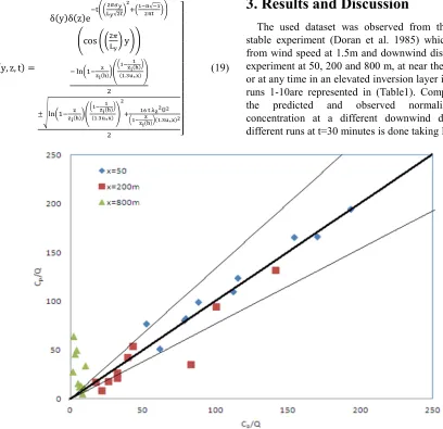
The used dataset was observed from the prairie Grass stable experiment (Doran et al. 1985) which was obtained from wind speed at 1.5m and downwind distance during the experiment at 50, 200 and 800 m, at near the surface at night or at any time in an elevated inversion layer in stable case for runs 1-10are represented in (Table1). Comparison between

the predicted and observed normalized integrated

concentration at a different downwind distance for the different runs at t=30 minutes is done taking Ly=100m.

Figure 1. Comparison between the predicted and observed normalized integrated concentration for three downwind distances 50, 200 and 800m respectively.

Table 1. Meteorological parameters and concentration measured during the prairie Grass stable experiment.

Run U (m/s) H (m) U* (m/s)

C/Q (10-4 _sm-2₎

observed Estimated

X=50m X=200m X=800m X=50m X=200m X=800m

1 3.63 325 0.24 88 32 10 99 21 28

2 3.63 325 0.11 170 141 27 166 132 64

3 3.63 325 0.1 193 100 41 194 94 46

4 3.63 325 0.29 61 21 7 51 9 50

5 3.63 325 0.28 78 26 8 80 18 16

6 1.42 135 0.14 112 39 - 110 42 12

7 1.42 135 0.11 115 43 17 124 54 13

8 1.42 135 0.23 79 32 12 82 26 5

9 1.42 135 0.37 52 17 5 77 17 11

10 1.42 135 0.17 154 83 32 165 35 34

Figure 1 shows the comparison between the predicted and observed normalized integrated concentration at different downwind distances at 50, 200, and 800 m. This Figure shows that the predicted two models at 50 and 200m are one to one and other inside a factor of two with the observed data while the third predicated model at 800m are inside a factor of three.

4. Statistical Method

FractionBias FB ŽC•− Cb•

‘0.5ŽC• Cb•“

NormalizedMeanSquareError NMSE ŽCb− C•• C

ŽCbC••

CorrelationCoefficient COR) 1

N•žŽCbW− Cb• ×

ŽC•W− C••

(σbσ•

¡

W¢c

FactorofTwo FAC2) 0.5 ≤C_Cb

•≤ 2.0

Where σp and σo are the standard deviations of Cp and Co respectively. Here the over bars indicate the average overall measurements.

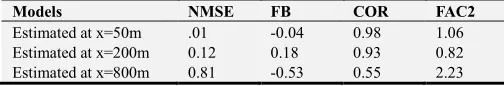
Table 2. Comparison between different models according to standard statistical performance measure.

Models NMSE FB COR FAC2

Estimated at x=50m .01 -0.04 0.98 1.06 Estimated at x=200m 0.12 0.18 0.93 0.82 Estimated at x=800m 0.81 -0.53 0.55 2.23

From this table, one finds that the two predicted models at 50 and 200m are inside the factor of two and the third model at 800m is inside a factor of three. Also the previous two present models are performance well for the observed data with respect to a normalized mean square error, fraction bias, and the correlation than the third present model.

5. Conclusion

Temporary diffusion equation is estimated by using separation variable method with eddy diffusivities measuring at near the surface at night or at any time in an elevated inversion layer in the stable condition to calculate normalized integrated concentration. The used dataset was observed from the “Project prairie Grass” (Barad 1958) which was obtained by wind speed at 1.5m and downwind distance during the experiment at 50, 200 and 800 m in stable case for runs 1-10. Comparison between the predicted and observed normalized integrated concentration at different downwind distances for the different runs at t= 30 minutes. The predicted data are one to one and other is inside a factor of two with observed data at 50 and 200m while the third predicated model at 800m is inside a factor of three. The statistical method shows that the two predicted models are inside a factor of two and the third predicted model is inside a factor of three. Also the previous two present models are performance well for the observed data with respect to a normalized mean square error, fraction bias, and the correlation than the third present model. Also the previous two predicted models are performance well for the observed data with respect to a normalized mean square error, fraction bias, and the correlation than the third predicted model.

Appendix

Appendix A

Using separation of variable method in the form: C (y, t) =G (y) F (t) in Eq. (5), one gets that:

§ ¨ § ¨ C G

§ ¨

§ ¨ L −λC A1

Dividing Eq. (A1) on G (y) F (t), one gets that:

¨ ¨ C G

§

§ L −λC (A2)

where λ is variable constant.

Equation (A2) is solved as follows:

F t) λ CF t) 0 (A3)

G y) C λ C_{G y) 0 (A4}

Integrating Eq. (A3 with respect to t from 0 to t, one gets that:

F t) c'eF ¬ (A5)

The solution of Eq. (A4) in the from:

G y) cccos QG√C λ L yT cCsin QG√C λ L yT (A6)

The general solution of C (y, t) is in the from:

C y, t) AeF ® _{cos QG}√C

¯ˆ ° L yT Bsin QG

√C

¯ˆ ° L yT (A7)

where A=c0c1 and B= c0c2

Substituting from (3) in (A7), one gets that:

A δ(y) (A8) Substituting from (4) in (A7), one gets that:

B 0 (A9) Substituting from (A9) in (A7), one gets that:

C y, t) δ(y)cos QG√C λ L yT (A10)

Substituting from (4) in (A10), one gets that:

G y) −δ(y)√C λ Msin QG√C λ L L TU (A11)

G√C_¯ˆ °L L 2µ → ° CŠ¯ˆ

S √C (A12)

C y, t) δ(y)eF Q

HI

@ √ KT _{Mcos QG}CR

S L yTU (A13)

Appendix B

Using separation of variable method in the form:

C (z, t) =M (z) N (t) (A14)

And Dividing Eq. (A14) on M (z) N (t)), one can get that:

k0 ¶·· 0

¶ 0 + k0 ¶· 0

¶ 0 −λC (A15)

Where “λ” is variable constant. Equation (A15) is solved as follows:

N t) −λ0CN t) (A16)

M··_(z) ¸9

¸9M

·_(z) ¬

¸9M(z) 0 (A17)

The solution of Esq.’s (A16) and (A17), one gets that:

N t) AeF¬9 _(A18)

M··_(z) ¸9

¸9M

·_(z) ¬9

¸9 M z ) =0 (A19)

Substation from (14) in (A18), one gets that:

A= δ (z) (A20)

Substation from (A20) in equation (A18), one gets that:

N t) δ(z) ¹F®º _(A21)

Where δ (z) is Dirac delta function in the form

δ(z) _CŠc ∑½ ¹v¼

¼¢F½ (Hazewinkel and et al. (2001)),

Substation from (12) in (A20).one gets that:

λ0 ¾cF8√Fc_CR (A22)

Integration Eq. (A19) with respect to "z" from 0 to z, one gets:

Mz)

F 78GcF_91(z)9 LlG>? >_{(>.g_∗€)}91(z)Lp

C

±‚78GcF_91(z)9 LlG>? >_{(>.g_∗€)}91(z)Lp < >ƒ K „9 …"

G>? 9_{91 z}L >.g_∗€)

C |

} } } } } ~

(A23)

Substation from Eq. (A21), (A23) in Eq. (A14), one gets that:

C(z, t)

δ(z) eF>?•√?>HK

F 78GcF_91(z)9 LlG>? >_{(>.g_∗€)}91(z)Lp

C

±‚78GcF_91(z)9 LlG>? >_{(>.g_∗€)}91(z)Lp < >ƒ K „9 …"

G>? 9_{91 z}L >.g_∗€)

C |

} } } } } } } ~

(A24)

References

[1] Akula Venkatram (2004): On estimating emissions through horizontal fluxes. Atmospheric Environment38, 1337-1344. [2] Barad M. L. (Ed) (1958). Project prairie Grass, A field

program in diffusion, vol. 1. Geophysics Research Paper no. 59, Geophysics Research Directorate, Air Force Cambridge Research Center.

[3] Doran J. C., and Horst T. W. (1985). ”An evaluation of Gaussian plume-depletion models with dual-tracer field measurement”. Atmos. Environ., 19, 939-951.

[4] Eckman, R. M., (1994). “Ro-examination of empirically derived formulas for horizontal diffusion from surface sources”. Atmospheric Environment: 28, 265-272.

[5] Hanna Steven R. Gary A. Briggs and Rayford P. hosker Jr. (1982). “Handbook on Atmospheric Diffusion”. Technical Information Center, U. S. Department of Energy.

[6] Hanna, S. R., 1989, “confidence limit for air quality models as estimated by bootstrap and Jacknife resembling methods”, Atom. Environ. 23, 1385-1395.

[7] Hazewinkel, Michiel, ed. (2001), “Delta-function”, Encyclopedia of Mathematics, Springer, ISBN 978-1-55608-010-4.

[8] John E. Till, Helen A. Grogan (2008). “Radiological risk assessment and environmental analysis”.

[9] Khaled S. M. Essa, Sawsan E. M. Elsaid and Fawzia Mubarak (2015).” Time dependent Advection-Diffusion Equation in Two Dimensions” Journal of Atmosphere, vol. 1, issue1, pages 8-16.

[10] Michael R. K. Thambynayagam, R. K. M (2011). The Diffusion Handbook: Applied Solutions for Engineers. McGraw-Hill.

[11] Palazzi, E., De Faveri, M., Fumarola, G., Ferraiolla, G., (1982), Diffusion from a steady source of short duration, Atmospheric Environment 16, 2785–2790.