Statistical Methods for High Dimensional Count and Compositional Data With Applications to Microbiome Studies

University of Pennsylvania

ScholarlyCommons

Publicly Accessible Penn Dissertations

1-1-2016

Statistical Methods for High Dimensional Count

and Compositional Data With Applications to

Microbiome Studies

Yuanpei Cao

University of Pennsylvania, [email protected]

Follow this and additional works at:

http://repository.upenn.edu/edissertations

Part of the

Applied Mathematics Commons, and the

Statistics and Probability Commons

This paper is posted at ScholarlyCommons.http://repository.upenn.edu/edissertations/1634

Recommended Citation

Cao, Yuanpei, "Statistical Methods for High Dimensional Count and Compositional Data With Applications to Microbiome Studies" (2016).Publicly Accessible Penn Dissertations. 1634.

Statistical Methods for High Dimensional Count and Compositional Data

With Applications to Microbiome Studies

Abstract

Next generation sequencing (NGS) technologies make the studies of microbiomes in very large-scale possible

without cultivation in vitro. One approach to sequencing-based microbiome studies is to sequence specific

genes (often the 16S rRNA gene) to produce a profile of diversity of bacterial taxa. Alternatively, the

NGS-based sequencing strategy, also called shotgun metagenomics, provides further insights at the molecular level,

such as species/strain quantification, gene function analysis and association studies. Such studies generate

large-scale high-dimensional count and compositional data, which are the focus of this dissertation.

In microbiome studies, the taxa composition is often estimated based on the sparse counts of sequencing

reads in order to account for the large variability in the total number of reads. The first part of this thesis deals

with the problem of estimating the bacterial composition based on sparse count data, where a penalized

likelihood of a multinomial model is proposed to estimate the composition by regularizing the nuclear norm

of the compositional matrix. Under the assumption that the observed composition is approximately low rank,

a nearly optimal theoretical upper bound of the estimation error under the Kullback-Leibler divergence and

the Frobenius norm is obtained. Simulation studies demonstrate that the penalized likelihood-based estimator

outperforms the commonly used naive estimator in term of the estimation error of the composition matrix

and various bacterial diversity measures. An analysis of a microbiome dataset is used to illustrate the methods.

Understanding the dependence structure among microbial taxa within a community, including co-occurrence

and co-exclusion relationships between microbial taxa, is another important problem in microbiome research.

However, the compositional nature of the data complicates the investigation of the dependency structure

since there are no known multivariate distributions that are flexible enough to model such a dependency. The

second part of the thesis develops a composition-adjusted thresholding (COAT) method to estimate the

sparse covariance matrix of the latent log-basis components. The method is based on a decomposition of the

variation matrix into a rank-2 component and a sparse component. The resulting procedure can be viewed as

thresholding the

sample centered log-ratio covariance matrix and hence is scalable to large covariance matrice estimations

based on compositional data. The issue of the identifiability problem of the covariance parameters is

rigorously characterized. In addition, rate of convergence under the spectral norm is derived and the

procedure is shown to have theoretical guarantee on support recovery under certain assumptions. In the

application to gut microbiome data, the COAT method leads to more stable and biologically more

interpretable results when comparing the dependence structures of lean and obese microbiomes.

Degree Type

Dissertation

Degree Name

Doctor of Philosophy (PhD)

Graduate Group

Mathematics

First Advisor

Hongzhe Li

Subject Categories

STATISTICAL METHODS FOR HIGH DIMENSIONAL COUNT AND COMPOSITIONAL DATA WITH APPLICATIONS TO MICROBIOME STUDIES

Yuanpei Cao

A DISSERTATION

in

Applied Mathematics and Computational Science

Presented to the Faculties of the University of Pennsylvania

in

Partial Fulfillment of the Requirements for the

Degree of Doctor of Philosophy

2016

Supervisor of Dissertation

Hongzhe Li

Professor of Biostatistics

Graduate Group Chairperson

Charles L. Epstein, Thomas A. Scott Professor of Mathematics

Dissertation Committee

STATISTICAL METHODS FOR HIGH DIMENSIONAL COUNT AND COMPOSITIONAL DATA

WITH APPLICATIONS TO MICROBIOME STUDIES

c

COPYRIGHT

2016

Yuanpei Cao

This work is licensed under the

Creative Commons Attribution

NonCommercial-ShareAlike 3.0

License

To view a copy of this license, visit

ACKNOWLEDGEMENT

I would like to first and foremost express my deepest gratitude to my advisor Professor Hongzhe Li

for the continuous support of my Ph.D study and research. With his extensive knowledge, sharp

thinking and enthusiasm about problems in biostatistics, he provided me with an excellent research

atmosphere and patiently guided me through a lot of difficulties during my Ph.D study.

I would also like to thank my thesis committee members, Professor Tony Cai and Professor

Zong-ming Ma. They gave me tremendous help and great suggestions on my scientific research and

presentation skills.

I would like to express my gratitude to my collaborators, Professor Wei Lin and Professor Anru

Zhang, for their stimulating discussions and inspiring comments.

My sincere thanks also go to Professor Charles Epstein, the graduate chair of Applied Mathematics

and Computational Science, for offering me this wonderful opportunity to pursue graduate studies

at Penn. I also want to thank my fellow graduate students and program coordinators for their

continuous support.

Last but not the least, I am deeply grateful to my wife Xin Feng as well as my parents for their love

and support all the time. Whenever I met with difficulties, they always gave me unconditional love

ABSTRACT

STATISTICAL METHODS FOR HIGH DIMENSIONAL COUNT AND COMPOSITIONAL DATA

WITH APPLICATIONS TO MICROBIOME STUDIES

Yuanpei Cao

Hongzhe Li

Next generation sequencing (NGS) technologies make the studies of microbiomes in very

large-scale possible without cultivationin vitro. One approach to sequencing-based microbiome studies

is to sequence specific genes (often the 16S rRNA gene) to produce a profile of diversity of

bac-terial taxa. Alternatively, the NGS-based sequencing strategy, also called shotgun metagenomics,

provides further insights at the molecular level, such as species/strain quantification, gene function

analysis and association studies. Such studies generate large-scale high-dimensional count and

compositional data, which are the focus of this dissertation.

In microbiome studies, the taxa composition is often estimated based on the sparse counts of

se-quencing reads in order to account for the large variability in the total number of reads. The first

part of this thesis deals with the problem of estimating the bacterial composition based on sparse

count data, where a penalized likelihood of a multinomial model is proposed to estimate the

compo-sition by regularizing the nuclear norm of the compocompo-sitional matrix. Under the assumption that the

observed composition is approximately low rank, a nearly optimal theoretical upper bound of the

estimation error under the Kullback-Leibler divergence and the Frobenius norm is obtained.

Simu-lation studies demonstrate that the penalized likelihood-based estimator outperforms the commonly

used naive estimator in term of the estimation error of the composition matrix and various bacterial

diversity measures. An analysis of a microbiome dataset is used to illustrate the methods.

Understanding the dependence structure among microbial taxa within a community, including

co-occurrence and co-exclusion relationships between microbial taxa, is another important problem in

microbiome research. However, the compositional nature of the data complicates the investigation

of the dependency structure since there are no known multivariate distributions that are flexible

enough to model such a dependency. The second part of the thesis develops a

log-basis components. The method is based on a decomposition of the variation matrix into a rank-2

component and a sparse component. The resulting procedure can be viewed as thresholding the

sample centered log-ratio covariance matrix and hence is scalable to large covariance matrice

estimations based on compositional data. The issue of the identifiability problem of the covariance

parameters is rigorously characterized. In addition, rate of convergence under the spectral norm

is derived and the procedure is shown to have theoretical guarantee on support recovery under

certain assumptions. In the application to gut microbiome data, the COAT method leads to more

stable and biologically more interpretable results when comparing the dependence structures of

lean and obese microbiomes.

The third part of the thesis considers the two-sample testing problem for high-dimensional

composi-tional data and formulates a testable hypothesis of composicomposi-tional equivalence for the means of two

latent log-basis vectors. A test for such a compositional equivalence through the centered log-ratio

transformation of the compositions is proposed and is shown to have an asymptotic extreme value

of type 1 distribution under the null. The power of the test against sparse alternatives is derived.

Simulations demonstrate that the proposed tests can be significantly more powerful than existing

tests that are applied to the raw and log-transformed compositional data. The usefulness of the

proposed tests is illustrated by applications to test for differences in gut microbiome composition

between lean and obese individuals and changes of gut microbiome between different time points

TABLE OF CONTENTS

ACKNOWLEDGEMENT . . . iii

ABSTRACT . . . iv

LIST OF TABLES . . . viii

LIST OF ILLUSTRATIONS . . . ix

CHAPTER 1 : COMPOSITION ESTIMATION FROM SPARSE COUNT DATA VIA A REGULAR-IZED LIKELIHOOD . . . 1

1.1 Introduction . . . 1

1.2 Poisson-Multinomial Model for Microbiome Count Data and Penalized Estimation . . 3

1.3 Optimization Algorithm and Tuning Parameter Selection . . . 5

1.4 Theoretical Properties . . . 10

1.5 Simulation studies . . . 14

1.6 Gut Microbiome Data Analysis . . . 17

1.7 Discussion . . . 19

CHAPTER 2 : LARGECOVARIANCEESTIMATION FORCOMPOSITIONALDATA VIA COMPOSITION-ADJUSTEDTHRESHOLDING . . . 21

2.1 Introduction . . . 21

2.2 Identifiability of the Covariance Model . . . 24

2.3 A Sparse Covariance Estimator for Compositional Data . . . 27

2.4 Theoretical Properties . . . 29

2.5 Simulation Studies . . . 32

2.6 Gut Microbiome Data Analysis . . . 39

2.7 Discussion . . . 42

CHAPTER 3 : TWO-SAMPLE MEAN TESTS FOR HIGH-DIMENSIONAL COMPOSITIONAL DATA. 44 3.1 A testable hypothesis of compositional equivalence . . . 46

3.3 Theoretical Results for theCLRTransformation-based Global Test . . . 49

3.4 Two-sample Test for Paired Observations . . . 53

3.5 Simulation Studies . . . 54

3.6 Real Data Analysis . . . 59

3.7 Discussion . . . 61

CHAPTER A : APPENDICES . . . 62

A.1 Additional Lemmas and Technical Proofs for Chapter 1 . . . 62

A.2 Additional Lemmas and Technical Proofs for Chapter 2 . . . 79

A.3 Additional Lemmas and Technical Proofs for Chapter 3 . . . 90

LIST OF TABLES

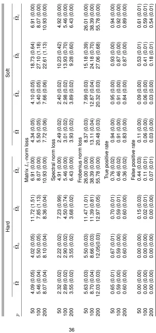
TABLE 2.1 : Means (standard errors) of various performance measures for four methods with hard and soft thresholding rules with normal-related distributions over 100 replications . . . 36 TABLE 2.2 : Means (standard errors) of various performance measures for four methods

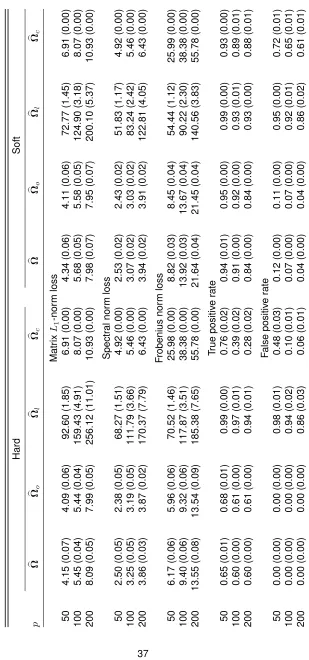
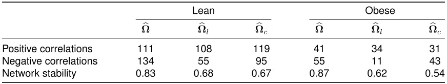
with hard and soft thresholding rules with gamma-related distributions over 100 replications . . . 37 TABLE 2.3 : Numbers of positive and negative correlations and stability of correlation

networks for three methods applied to the gut microbiome data . . . 40

TABLE 3.1 : Empirical size and power of the tests based on 1000 replications withα= 0.05andn = 100for basis generated from log-normal distributions. Model 1: α1 = α2 = 3, α3 =α4 = 10,β1 = β2 = 0.05. Model 2: α1 =α2 = 10, α3 =α4 = 20,β1= 0.15,β2 = 0.2. Model 3:α1 =α2= 10,α3=α4 = 20, β1 = 0.05, β2 = 0.1. Model 4: α1 = α2 = 10, α3 = α4 = 20, β1 = 0.15, β2= 0.2. . . 57 TABLE 3.2 : Empirical size and power of tests based on 1000 replications withα= 0.05

andn = 100for basis generated from log-Gamma models. Model 1: α1 = α2 = 3,α3 =α4 = 10,β1 =β2 = 0.05. Model 2: α1=α2 = 10,α3 =α4=

LIST OF ILLUSTRATIONS

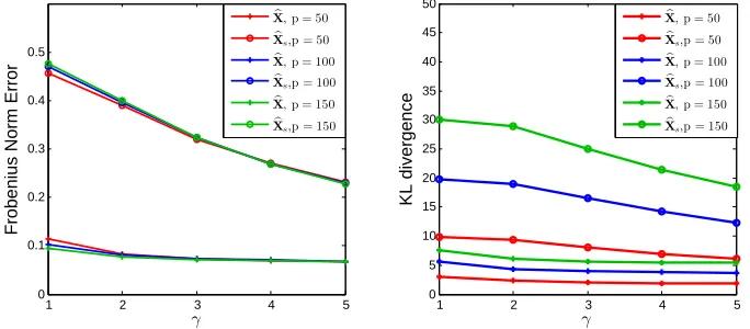
FIGURE 1.1 : Frobenius norm error and Kullback-Leibler divergence between the esti-mated and the true compositions for different numbers of taxapin Model 1, whereXb is the proposed estimator andXbsis the estimator with simple

zero replacement. . . 15 FIGURE 1.2 : Frobenius norm error and Kullback-Leibler divergence between the

esti-mated and the true compositions for different numbers of taxapin Model 2, whereXb is the proposed estimator andXbsis the estimator with simple

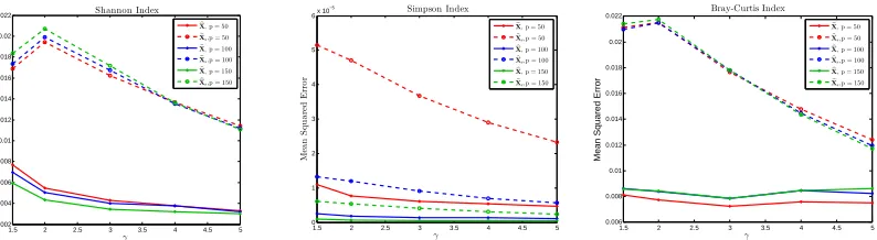
zero replacement. . . 16 FIGURE 1.3 : Losses on different diversity indices between the estimated and the true

compositions for different numbers of observed taxa pin Model 1. Left panel: Shannon index; Middle panel:Simpson index; Right panel: Bray-Curtis index . . . 16 FIGURE 1.4 : Losses on different diversity indices between the estimated and the true

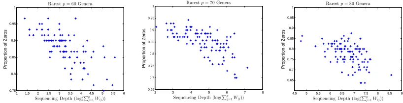
compositions for different numbers of observed taxa pin Model 2. Left panel: Shannon index; Middle panel:Simpson index; Right panel: Bray-Curtis index . . . 17 FIGURE 1.5 : Proportions of zeros observed versus the size library sizes, indicating that

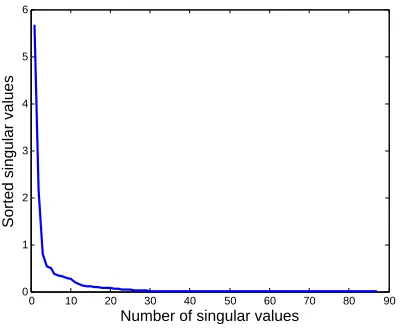
many observed zeros are due to under sampling. . . 17 FIGURE 1.6 : Decay of singular valuesdiifrom the SVD decomposition ofX=UDVT. 18

FIGURE 1.7 : Boxplots of the estimated compositions for each genus for those with zero observations (M) and those with non-zero observations (Mc_{). Top panel:}

proposed estimatorXb; Bottom panel: estimator with zero-replacementXbs. 19

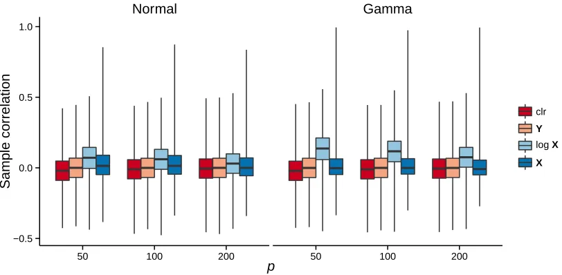
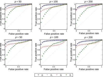
FIGURE 2.1 : Boxplots of sample correlations with simulated data under different trans-formations in Model 1. . . 34 FIGURE 2.2 : ROC curves for four methods in Model 2 with normal-related distribution

(top panel) and gamma-related distribution (bottom panel). . . 38 FIGURE 2.3 : Correlation networks identified by the COAT method for the lean and obese

groups in the gut microbiome data. Positive and negative correlations are displayed in green and red, respectively. The thickness of edges indicates the magnitude of correlations. . . 41

CHAPTER 1

C

E

S

C

D

R

L

In microbiome studies, taxa composition is often estimated based on the sequencing read counts

in order to account for the large variability in the total number of observed reads across different

samples. Due to sequencing depth, some rare microbial taxa might not be captured in the

metage-nomic sequencing, which results in many zero read counts. Naive composition estimation using

count normalization therefore lead to many zero proportions, which underestimates the underlying

compositions, especially for the rare taxa. Such an estimate of the composition can further lead

to biased estimate of taxa diversity, and can also cause difficulty in downstream log-ratio based

analysis for compositional data. In this paper, the observed counts are assumed to be sampled

from a multinomial distribution, with the unknown composition being the probability parameter in

a high dimensional positive simplex space. Under the assumption that the composition matrix is

approximately low rank, a nuclear norm regularization-based likelihood estimation is developed

to estimate underlying compositions of the samples. The theoretical upper bounds and the

min-max lower bounds of the estimation errors measured by the Kullback-Leibler divergence and the

Frobenius norm are established. Simulation studies demonstrate that the regularized maximum

likelihood estimator outperforms the commonly used naive estimators. The methods are applied to

an analysis of a human gut microbiome dataset.

1.1. Introduction

The human microbiome is the totality of all microbes at different body sites, whose contribution to

human health and disease has increasingly been recognized. Recent studies have demonstrated

that the microbiome composition varies across individuals due to different health and the

environ-ment status (The Human Microbiome Project Consortium, 2012a), and may be associated with

complex diseases such as obesity, atherosclerosis, and Crohn’s disease (Koeth et al., 2013; Lewis

et al., 2015; Turnbaugh et al., 2009). With the development of next-generation sequencing

tech-nologies, the human microbiome organisms can be quantified by using direct DNA sequencing of

refer-ence microbial genomes, the observed count data (e.g., 16S rRNA marker gene reads or shotgun

metagenomic reads) depend on the amount of genetic material extracted from the community or

the sequencing depth, and they provide a relative measure of the abundances of community

com-ponents. In a microbiome study, these read counts are typically non-negative and over-dispersed,

and contain a large number of zeros.

In order to account for the large variability in the total number of reads obtained, the taxa

compo-sition is often estimated based on the observed counts of sequencing reads. Due to sequencing

depth, some rare microbial taxa might not be captured in the metagenomic sequencing, which

re-sults in zero read counts assigned to these taxa. Naive estimates of the taxa composition using

count normalization therefore lead to many zeros due to under sampling, especially for rare taxa.

Such a naive estimate of the composition can be biased and can lead to biased estimates of taxa

diversity. It can also cause difficulty in downstream data analysis for compositional data. Since the

pioneering work of Aitchison, (2003), several techniques have been proposed to deal with zeros

(see Martın-Fernandez, Palarea-Albaladejo, and Olea, 2011 for an overview) in count data. One

approach is to replace zero counts through a Bayesian-multiplicative model, followed by

normaliz-ing the count into the composition. Such a Bayesian method involves a Dirichlet prior distribution

as the conjugate distribution of multinomial distribution and a multiplicative modification of the

non-zero counts. The non-zero replacement results were determined by the parameterizations of the prior

distribution. However, such a prior information cannot be easily obtained, and the subjective

selec-tion of the parameter may yield misleading results. Other approaches normalized the count first and

treated zero compositions as the missing values. The missing part was then recovered by either

non-parametric imputation or EM algorithms. However, the non-parametric imputation lacks

theo-retical guarantees for selecting a reasonable replacement value. The EM algorithm is not feasible

when the number of taxa is very large, or every taxa contains at least one zero across the samples.

In addition, the multivariate additive log-ratio (alr) normality assumption used in these methods is

number of total count is a Poisson random variable. If the compositions across different individuals

are treated as a matrix by combining them together, an approximately low rank structure on this

matrix is indicated by recent observations on co-occurrence pattern (Faust et al., 2012) and various

symbiotic relationships in microbial communities (Chaffron et al., 2010; Horner-Devine et al., 2007;

Woyke et al., 2006). Motivated by much success in solving the matrix completion problem using

nuclear norm minimization (Cao and Xie, 2016; Klopp et al., 2015; Lafond et al., 2014; Lu and

Ne-gahban, 2014; Negahban and Wainwright, 2012), this paper solves the problem of the composition

estimation using a regularized maximum likelihood approach. However, it should be emphasized

that the multinomial likelihood function in this framework has not been studied and the sampling

scheme used in this article is also different from other matrix completion problems. The observed

zero counts are the result of under sampling, rather than the random missingness assumed in the

previous literature. We provide the asymptotic upper and min-max lower bounds of the resulting

regularized estimator and show through simulations that the estimator recovers low-rank

composi-tions accurately.

The rest of the paper is organized as follows. Section1.2presents details of the proposed

regu-larized likelihood approach when the underlying composition is approximately low-rank. The

imple-mentation is presented in Section 1.3. The theoretical properties of the estimators are analyzed in

Section1.4, where the upper bounds for the estimation error measured by average Kullback-Leibler

divergence and Frobenius norm are established. Simulation results are shown in Section1.5to

in-vestigate the numerical performance of the proposed methods. A real data application to a human

gut microbiome study is given in Section1.6.

1.2. Poisson-Multinomial Model for Microbiome Count Data and Penalized

Estima-tion

In this section, we consider a Poisson-multinomial statistical model for composition estimation from

the sparse count data observed in microbiome studies. The proposed procedure for composition

estimation relies on a regularized maximum likelihood. We start by introducing some notation that

will be used throughout the rest of the paper. For any integersN > 0, let[N] = {1,2,· · · , N}be

the set of integers ranging from 1 toN. We also denote1n = (1, . . . ,1)> ∈Rn,eias the canonical

vector if u≥ 0 andPp

i=1ui = 1. For any two composition vectorsu, v ∈ Rp, we can define the

Kullback-Leibler (KL) divergence as

DKL(u, v) = p

X

j=1 uilog

ui

vi

. (1.1)

For any matrix A = (aij), define itsL1, L∞, spectral, Frobenius, element-wise maximum, and

nuclear norm respectively askAk1,kAk∞,kAk2,kAkF,kAkmax, andkAk∗. Specifically,kAk1=

max

j

P

i|aij|,kAk∞= max

i

P

j|aij|,kAk2=

p

λmax(ATA),kAkF =

q P

i,ja2ij,kAkmax= max

i,j |aij|,

andkAk∗ =Piσi(A), whereλmax(·)denotes the largest eigenvalue and{σi(·)}denotes the set

of singular values. For two matricesAandB, lethA,Bi= tr(ATB) =P

i,jaijbijbe the trace inner product. Finally, for notational simplicity, we useC1, C2, . . .as generic symbols for constants whose

values may vary from line to line.

Our starting point is an×pmatrix of countsWwith elementWij representing the observed read

count of taxonj in individual i, wherei ∈ [n] andj ∈[p]. For i-th individual, the simplest model

for their count dataWi = (Wi1, Wi2,· · · , Wip)is the multinomial model with its probability function

given as

fM(Wi1, Wi2,· · ·, Wip;Xi) =

Ni

Wi

p

Y

j=1

X_ij∗Wij_,

where Ni = P p

j=1Wij and X∗i = (Xi∗1, Xi∗2,· · ·, Xip∗) are underlying bacterial composition with

Pp

j=1X

∗

ij = 1, Xij∗ >0. The total taxa countNiis determined by the sequencing depth and can be

treated as a Poisson random variable given byNi ∼Pois(νi), whereνiis a positive parameter, but

it is of less interest.

Our goal is to estimate X∗ = (X∗₁T,X∗₂T,· · · ,X∗_pT)T _{based on W. The most natural estimate}

is obtained by the maximum likelihood estimation. Denote by LN the (normalized) negative

positive simplex spaceS ={X∈_Rn×p

X1p=1n,X>0}. Without further constraints, minimizing

(1.2) leads to the standard maximum likelihood estimateXb,

b

Xij =

Wij

Pp

k=1Wik

, i∈[n], j∈[p].

However, as a consequence of under sampling whenNis not sufficiently large, the estimatorXb will

contain a large number of zeros. These zeros underestimate the composition and cause difficulty in

downstream log-ratio based compositional data analysis (Aitchison, 2003). For an arbitrary matrix

X∗ _{in positive simplex space, clearly there is no good way to recover a positive X}∗_{. However, in}

the metagenomic study,X∗could be approximately low-rank in the sense that the singular values

decay gradually towards zero, which provides the possibility to recover X∗ with high accuracy.

In this paper, we propose a penalized estimator Xb based on a regularized maximum likelihood

formulation:

b

X= arg min

X∈S(αx,βx)

LN(X) +λkXk∗, (1.3)

whereS(αx, βx)is a bounded simplex space given by

S(αx, βx) =

X∈Rn×p

X1p=1n, αx/p≤Xij≤βx/p,∀(i, j)∈[n]×[p]

.

Hereλandαxandβxare tuning parameters. The constrained element-wise lower bound

guaran-tees the positive sign of the estimator. The element-wise upper bound constraint is only needed in

the theory, while in practice, such a constraint is not required.

1.3. Optimization Algorithm and Tuning Parameter Selection

In this section we consider the implementation of the proposed estimator specified as (1.3).

Specif-ically, we propose to solve the following constrained convex optimization:

b

X= arg min

X∈S(αX)

LN(X) +λkXk∗, (1.4)

S(αX) =

X∈Rn×p

X1p =1n, Xij ≥αX/p,∀(i, j)∈[n]×[p]

HereS(αX)is a positive simplex space and(λ, αX)is a pair of tuning parameters. Particularly, (1.4)

is a nuclear norm minimization problem, which can be solved by either semidefinite programing via

interior-point SDP solver, or first-order method via Templates for First-Order Conic Solvers

(TFOC-S), see Becker, Cand `es, and Grant, 2011. However, the SDP solver computes the nuclear norm

via a less efficient eigenvalue decomposition which does not scale well with high-dimensionsnand

p. Besides, Nesterov’s scheme used in TFOCS is not monotone in the objective function owing

to the introduction of the momentum term, which often results in oscillations or overshoots along

the trajectory of the iteration. In this article, we propose a more efficient algorithm based on the

generalized accelerated proximal gradient method (Su, Boyd, and Candes, 2014). To adapt to the

bounded simplex constraintS(αX), we develop a non-iterative projection scheme in the proposed

algorithm.

1.3.1. Generalized Accelerated Proximal Gradient Method

SinceLN(·)is convex and differentiable over the domainS(αX)and the nuclear norm is convex, the

accelerated Nesterov’s scheme can be formulated as follows. Given the count matrixW, we first

normalize it into the compositionXby Xij =Wij/Pp_k=1Wikand initializeY0 =X0 =X−1 =X,

then updateXk andYkin thekth iteration as

Xk = arg min

X∈S(αX) Lk

2 kX−Yk−1+L

−1

k OLN(Yk−1)k2F+λkXk∗, (1.5)

Yk =Xk+

k−1

k+r−1(Xk−Xk−1). (1.6)

Here we provide the detailed explanation for (1.5) and (1.6).

• Lk is the step size in thek-th iteration, which is chosen by line search strategy. Denote by

FL(X,Y)the approximation error when approximating LN(X) with its second order Taylor

expansion aroundYand usingLas the second order coefficient,

FL(X,Y) =LN(X)− LN(Y)− hX−Y,OLN(Y)i −

L

2kX−Yk

2

• k−1

k+r−1 is the momentum term andris a friction parameter. In the standard accelerated gradi-ent method, the friction parameter is set byr= 3, and this scheme exhibits the convergence

rateO(1/k2_{)as long as the gradient function}

OLN is Lipschitz continuous with a constant

Lip-schitz coefficient (Nesterov, 1983, 2013). The Nesterov’s scheme can be further generalized

by setting a high friction rate, for example r ≥9/2, and it succeeds in eliminating the

over-shooting and oscillation along the trajectory toward the minimizer and obtaining a O(1/k3₎

convergence rate (Su, Boyd, and Candes, 2014).

• The minimization of the objective function (1.5) can be solved by a form of Singular Value

Thresholding (SVT) (Cai, Cand `es, and Shen, 2010):

Xk= ΠS(αX)

D_λL−1

k

Yk−1−L−k1OLN(Yk−1)

.

HereΠ_S(αX)(X)is Euclidean projection ofXonto the positive simplex spaceS(αX)that we

will discuss in Section 1.3.2. If X= UΣVT _{is the singular value decomposition (SVD), the}

soft-thresholding operatorDτ can be defined as

Dτ(X) =UDτ(Σ)VT, Dτ(Σ) = diag (max{σi−τ,0}).

Combining these steps together, the generalized accelerated proximal gradient method is

sum-marized in Algorithm1, where kmax is the maximum number of iteration. The complexity of the

algorithm are dominated byO(n2_p+p3_{), which is the cost of singular value decomposition. The}

convergence of Algorithm 1 cannot be easily established; however, the following proposition

pro-vides some insight.

Proposition 1. Let Xk be the sequencing generated in the iteration of Algorithm 1. Denote by

f(X) =LN(X) +λkXk∗. Suppose the Euclidean projection onto the simplex spaceΠS(αX) does

not influence the convergence rate, and the step size is always set byLk = max

ij Wijp/(αXN).

Then, for any friction parameterr≥9/2, we have,

f(Xk)−f(X?)≤C

v u u u t

max

ij W

3

ij

min

{ij|Wij>0} Wij

p3

N2

kX0−X?k2F

whereX?is any minimizer off andConly depends onrandαX.

Since the gradient functionOLN is Lipschitz continuous with the constantL = max

ij Wijp/(αXN)

and the negative likelihood function LN is µ−strongly convex with µ = min

{ij|Wij>0}

Wij/N on the

constrained simplex space, it is not hard to prove Proposition 1 by applying Theorem 9 in Su, Boyd,

and Candes, 2014. The parametersLandµvary with different observations, as a result, the rate of

convergence shows an interesting dependency on the dimensionpand the observation countW

Algorithm 1Generalized accelerated proximal gradient method

1: Input: CountWand its normalized compositionX

2: Initialize:Y0=X0=X−1=X,r≥9/2,γ >1,L= 10−4, andkmax∈N+

3: fork= 1tokmax do

4: Xk= ΠS(αX) Dλ/L(Yk−1−(1/L)OLN(Yk−1))

5: if FL(Xk,Yk−1)≥0,then 6: L=γL, go to Step 3

7: end if

8: UpdateYk =Xk+_k+k−_r−1₁(Xk−Xk−1) 9: if|FL(Xk,Yk−1)|<10−5then

10: returnXk

11: end if

12: end for

1.3.2. Euclidean Projection onto the Simplex Space

The remaining part is to deal with the Euclidean projection onto the simplex spaceS(αX)in

Algo-rithm 1. We introduce a non-iterative and efficient algoAlgo-rithm based on the standard KKT condition.

Consider a one-dimensional simplex projection problem given by

ΠS(αX)(y) = min_x∈

Rp

1

2kx−yk

2 2 s.t.

p

X

i=1

xi= 1, xi≥αX/p. (1.7)

The following Proposition provides an implicit formulation for the minimizerx? to this optimization

problem (1.7).

Proposition 2. Suppose thaty1≥y2≥ · · · ≥yp, then the minimizerx?= (x1, x2,· · ·, xp)T is given

larger thanαX/p. We establish the the following formulation forρ,

ρ= max

(

j∈[p]

yj+j−1(1−αX− j

X

i=1 yi)>0

)

.

In the multi-dimensional case thatY∈Rn×p, we generalize the above simplex projection and

sum-marize this non-iterative optimization procedure in Algorithm2. The scheme is easy to implement

and its complexity isO(nplog(p)).

Algorithm 2Euclidean projection of a matrix onto the simplex spaceS(αX).

1: Input: Y∈Rn×pandS(αX)

2: Sort each row ofYintoU:Ui1≥Ui2· · · ≥Uip, i∈[p].

3: Find vectorρ= (ρ1,· · ·, ρn)T such that

ρi= max

(

j∈[p]

Uij+j−1 1−αX−

j

X

i=1 Uij

!

>0

)

, i∈[n].

4: Define vectorµ= (µ1,· · · , µn)T byµi=ρi−1

1−αX−Pρ_ji₌₁Uij

+αX/p, i∈[n].

5: ReturnXsuch thatXij = max{Yij+µi, αX/p},(i, j)∈[n]×[p].

1.3.3. Data Driven Selection of the Tuning Parameters

The proposed nuclear norm minimization involves the tuning parametersλandαX. We propose

the following data-driven method for selecting these tunning parameters with a guaranteed

per-formance. Given a selected parameter αX, we choose λ = λ(αX,βbR)by plugging αX and the

estimated row probability parameter

b

βR=n· max

1≤i≤n

Pp

j=1Wij

Pn

k=1

Pp

l=1Wkl

λ(αX,βbR) =

v u u t32

b

β2

R/n+ (1∨βbRp/n)/αX

plog(n+p)

N ∨

8(1/αX+βbR/(np)1/2)nlog(n+p)

N .

This choice ofλis motivated by the theoretical results of Theorem 1 in the next Section.

It remains to find the estimated parameterαX, which can be selected usingK-fold cross-validation

t∈T, set

(λ, αX) = (λ(αX(t),βbR), αX(t)) = (λ((t·αbX),βbR), t·αbX),

where

b

αX =p· min

1≤i≤n,1≤j≤p

Wij

Pn

k=1

Pp

l=1Wkl

andβbR=n· max

1≤i≤n

Pp

j=1Wij

Pn

k=1

Pp

l=1Wkl

.

We randomly split the rows ofWinto two groups of sizesn1∼ (K−1)n

K andn2∼ n

K forItimes. We

used the second group with sample sizen2as the testing set. In order to estimate the composition

from the rows in testing set, we further randomly picked1/K proportion of observed columns in

each row from the second group and combined it with the first group as the training set. Denote

by Wi _{be the selected testing set in the ith split and let X}i _{be its compositions through X}i kl =

Wi

kl/

Pp

l=1W

i

kl. Denote byXb(−i)(αX(t))the estimator based on the training set. We consider the

Kullback-Leibler divergence to evaluate the prediction error.

b

R(t) =

I

X

i=1

D(Xi,Xb(−i)(αX(t))).

We select t∗ = arg minTRb(t)and choose the tuning parameters (λ(αX(t∗),βbR), αX(t∗)). If t∗ is

chosen on the boundary ofT, we expand the range ofT and repeat the above procedure. With the

chosen tuning parameters, we finally obtain estimate by solving (1.4) based on the full dataset.

1.4. Theoretical Properties

We prove that the proposed estimator Xb achieves the near optimal rate of convergence over a

class of low-rank compositions. The regularization assumptions we need for theoretical analysis

are formally stated as below.

Condition 1. LetRi =νi/P

p

j=1νj fori∈[n], then there exist constants(αR, βR)such that, for any

i∈[n],

αR/n≤Ri≤βR/n.

Here R = (R1,· · ·, Rn)T represents the probability of observing an element from each row, and

Xrepresents the column probability. Conditions 1 and 2are analogous to the incoherence

con-ditions that are commonly assumed in the matrix completion literature. The element-wise upper

bounds avoid the overly ”spiky” situation that some rows or columns are sampled with very high

probability. The element-wise lower bound onRhelps to establish bounds in Frobenius norm, and

the entry-wise bound onX∗ensure the gradient function ofLN(X)in (1.2) is Lipschitz continuous,

which helps to effectively bound Frobenius norm in terms of Kullback-Leibler (KL) divergence and

guarantee the feasibility of accelerated gradient descent algorithm in practice.

1.4.1. Rate of Convergence

To assess how close the estimatorXb from (1.3) to the real compositional matrixX∗, we use average

Kullback-Leibler divergenceD(X∗_, b

X)and squared Frobenius normkX∗₋ b

Xk2

F. HereD(X∗,Xb)is

defined as the sum of Kullback-Leibler (KL) divergence between rows ofX∗andXb,

D(X∗,Xb) =

n

X

i=1

DKL(X∗i,Xbi) = n

X

i=1

p

X

j=1

X_ij∗logX

∗

ij

b

Xij

.

The following theorem gives an upper bound on the loss of the proposed estimator X∗ for the

exactly low-rank composition matrixX.

Theorem 1. (Exactly low-rank matrices)Under Conditions 1 and2, suppose thatN ≥ c0(n∨

p) log(n+p)for some universal constantc0>0, and the tuning parameter is selected as

λ= 2

r

C1(n, p)plog(n+p)

N ∨

C2(n, p)plog(n+p) N

!

, (1.8)

whereC1(n, p) = 8 βR2/n+ (1∨βRp/n)/αX

andC2(n, p) = 4(1/αX+βR/(np)1/2). If the

compo-sitionX∗ has rank at mostr, then, with probability at least1−3(n+p)−1_{, the estimate}

b

Xin(1.3)

satisfies

1

nD(X

∗_, b

X)≤C1

_{(p+n)rlog(n+p)}

N

, (1.9)

p

nkXb −X

∗_k2

F ≤C2

_{(p+n)rlog(n+p)}

N

, (1.10)

Theorem 1 states the rate of convergence for both KL divergence and Frobenius loss in terms

of probability. With some additional mild assumptions, the same rate of convergence holds in

expectation.

Corollary 1. Under the same conditions mentioned in Theorem 1, ifNfurther satisfiesN≤c1(n+

p)2_{rlog(n+p), then, there exists some constants C}

1 andC2 only depending onc0, c1, αX, βX, αr

andβR, such that

1

nED(X

∗_, b

X)≤C1

(p+n)rlog(n+p)

N ,

p

nE

Xb −X

∗

2

F ≤

C2

(p+n)rlog(n+p)

N .

We also have the corresponding lower bound that shows that the bound in Theorem1essentially

cannot be improved.

Theorem 2. Consider the matrix classes

B0(r, α, β) =

X∈Rn×prank(X)≤r,X1p=1n, α/p≤Xij ≤β/p, for any(i, j)∈[n]×[p] .

If2≤r≤p/2, there exists some constantsC1andC2which only depend onαX, βX, αR, βR, such

that

inf

b

X

sup

X∗∈B0(r,αX,βX)

αR≤Ri≤βR 1

nED(X

∗_, b

X)≥C1

(p+n)r

N ,

inf

ˆ

X

sup

X∗∈B0(r,αX,βX)

αR≤Ri≤βR p

nE

Xb −X

∗

2

F ≥C2

(p+n)r

N .

In practice, the composition is typically approximately low-rank instead of exactly low-rank. In such

case, we formalize the class of approximately low-rank matrices via thelq-”ball” of matrices by

Bq(ρq) =

(

X∈Rn×p

n∧p

X

|σi(X∗)|

q

≤ρq,

)

the compositionX∗ further belongs to a class of approximately low-rank matrices, Then, with the

probability proceeding1−3(n+p)−1_{, the estimator}

b

Xin(1.3)satisfies

1

nD(X

∗_, b

X)≤C1ρq(p/n)

q

2

_{(n+p) log(n+p)}

N

1−q2

, (1.12)

p

nkXb −X

∗_k2

F ≤C2ρq(p/n)

q

2

_{(n+p) log(n+p)}

N

1−q2

, (1.13)

where constantsC1andC2only depend onc0, αX, βX, αRandβR.

1.4.2. Estimation of Diversity Index

Various microbial diversity meaures are aften used to quantify the composition of the microbial

communities. GivenX∈Rp that representsp-bacteria composition acrossndifferent individuals,

three widely used measurements of microbial community diversity include

• Shannon’s index Hsh(Xi) =−P p

j=1XijlogXij,1≤i≤n;

• Simpson’s index H_sp(Xi) =P p j=1X

2

ij,1≤i≤n;

• Bray-Curtis index H_bc(Xi,Xj) =P p

k=1|Xik−Xjk|/2,1≤i, j≤n.

Here {H_sh(Xi)}ni=1 and {Hsh(Xi)}ni=1 are two vectors in which each component measures the

richness and evenness of microbial community in an individual;{Hbc(Xi,Xj)}n,pi,j=1is a matrix with

each entry ranging from[0,1]that quantifies the dissimilarity between two individuals. Higher value

of Bray-Curtis index indicates that two microbial communities are less likely to share similar taxa.

The penalized likelihood estimatorXb from (1.3) can be used to estimate Shannon’s, Simpson’s and

Bray-Curtis indices. The following Corollary provides the upper bound of these estimates.

Corollary 2. Under Conditions1and2, suppose thatN ≥c0(n∨p) log(n+p)for some constant

c0, and the tuning parameter is selected by (1.8). If the compositionX∗ has rank at mostr, then

the estimateXb in (1.3) satisfies

1 n

n

X

i=1

(Hsh(Xbi)−Hsh(X∗i))

2_=O

p

_(n+p)(logp)2_rlog(n+p) N

,

1 n

n

X

i=1

(Hsp(Xbi)−Hsp(X∗i))

2_=O

p

_{(n+p)rlog(n+p)}

p2_N

,

1 n2

X

1≤i<j≤n

(Hbc(Xbi,Xbj)−Hbc(X∗i,X

∗

j))

2_=O

p

(n+p)rlog(n+p) N

If the compositionX∗belongs the class of approximately low-rank matrices (1.11), then the estimate

b

Xin (1.3) satisfies

1 n

n

X

i=1

(H_sh(Xbi)−Hsh(X∗i))

2_=O

p ρq(logp)2(p/n)

q

2

_{(n+p) log(n+p)}

N

1−q2!

,

1 n

n

X

i=1

(Hsp(Xbi)−Hsp(X∗i))

2

=Op ρqp

q

2−2_/n

q

2

_{(n+p) log(n+p)}

N

1−q2!

,

1 n2

X

1≤i<j≤n

(Hbc(Xbi,Xbj)−Hbc(X∗i,X

∗

j))

2_=O

p ρq(p/n)

q

2

(n+p) log(n+p) N

1−q₂!

.

1.5. Simulation studies

Simulations studies were performed to evaluate the proposed composition estimatorXb and to

com-pare the results with the naive estimatorXbsthat replaces zero count with the maximum rounding

error 0.5 (Aitchison, 2003) and transforms the counts into composition.

1.5.1. Simulation settings

Data (X∗,R) were generated as follows. The row probability vector{Ri}ni=1 was generated as

the normalization of i.i.d entries {Pi}ni=1 uniformly drawn from Unif[1,10]: Ri = Pi/P n

k=1Pk. In

order to generate the compositionX∗, we first generated a rank-rmatrixZbyZ =UVT_{, where}

U ∈ Rn×r andV ∈ Rp×r. The components in Uare the absolute values of i.i.d N(0,1) normal

random variables. V = V1+V2 is a spike matrix, where the diagonal elements ofV1 are ones

and off-diagonal entries are equal to 1 with the probability 0.3 and equal to 0 with the probability

0.7, and the entries ofV2are independentN(0,10−3)normal random variables. This procedure is

repeated until we obtain a strict positive matrixZ. The following two models are considered forr.

• Model 1 (Exactly low rank):r= 20.

• Model 2 (Approximately low rank): r=n∧p.

ThenX∗ was obtained through the normalizationX∗ =Z /Pp _Z

1.5.2. Composition Estimate

We applied the penalized maximum likelihood approach to simulated data in both low rank and

approximately low rank cases. The tuning parameters(λ, αX)in each estimator were chosen by

five-fold cross-validation. For comparison, we calculated the naive estimators Xbs that replaced

zero counts by 0.5 and converted the counts into composition. Losses under squared Frobenius

normkXb −X∗k_F2 and Kullback-Leibler divergenceD(X∗,Xb)were used to measure the estimation

performance.

The simulation results for Model 1 and 2 are summarized in Figures1.1 and1.2respectively. We

observed that the proposed estimator Xb resulted in uniformly smaller errors thatn those based

on the naive estimatorXbsin all settings, demonstrating the superiority of the penalized likelihood

estimation. In addition, as expected, the difference in the loss ofXb and that ofXbsgot smaller as the

total counts increased since the number of zeros decreased as more read counts were observed.

1 2 3 4 5

0 0.1 0.2 0.3 0.4 0.5

γ

Frobenius Norm Error

b

X, p = 50 b

Xs,p = 50

b

X, p = 100 b

Xs,p = 100

b

X, p = 150 b

Xs,p = 150

1 2 3 4 5

0 5 10 15 20 25 30 35 40 45 50

γ

KL divergence

b

X, p = 50 b

Xs,p = 50

b

X, p = 100 b

Xs,p = 100

b

X, p = 150 b

Xs,p = 150

Figure 1.1: Frobenius norm error and Kullback-Leibler divergence between the estimated and the true compositions for different numbers of taxapin Model 1, whereXb is the proposed estimator

1 2 3 4 5 0 0.1 0.2 0.3 0.4 0.5 γ

Frobenius Norm Error

b

X, p = 50 b

Xs,p = 50

b

X, p = 100 b

Xs,p = 100

b

X, p = 150 b

Xs,p = 150

1 2 3 4 5

0 5 10 15 20 25 30 35 40 45 50 γ KL divergence b

X, p = 50 b

Xs,p = 50

b

X, p = 100 b

Xs,p = 100

b

X, p = 150 b

Xs,p = 150

Figure 1.2: Frobenius norm error and Kullback-Leibler divergence between the estimated and the true compositions for different numbers of taxapin Model 2, whereXb is the proposed estimator

andXbsis the estimator with simple zero replacement.

1.5.3. Diversity Index Estimate

To evaluate the ability to estimate the individual-level diversity and dispersion, we also calculated

vector L2 norm losses of the Shannon index and Simpson index, as well as the Frobenius norm

error of Bray-Curtis index. The simulation results for both models are summarized in Figures1.3

and1.4. We see that the proposed estimatorXb uniformly outperformed the naive estimatorsXbsby

a large margin.

1.5 2 2.5 3 3.5 4 4.5 5 0.002 0.004 0.006 0.008 0.01 0.012 0.014 0.016 0.018 0.02 0.022 γ M ea n S q u a re d E rr o r Shannon Index b

X, p = 50

b

Xs,p = 50

b

X, p = 100

b

Xs,p = 100

b

X, p = 150

b

Xs,p = 150

1.5 2 2.5 3 3.5 4 4.5 5 0 1 2 3 4 5 6x 10

−5 γ M ea n S q u a re d E rr o r Simpson Index b

X, p = 50

b

Xs,p = 50

b

X, p = 100

b

Xs,p = 100

b

X, p = 150

b

Xs,p = 150

1.5 2 2.5 3 3.5 4 4.5 5 0.006 0.008 0.01 0.012 0.014 0.016 0.018 0.02 0.022 γ

Mean Squared Error

Bray-Curtis Index

b

X, p = 50

b

Xs,p = 50

b

X, p = 100

b

Xs,p = 100

b

X, p = 150

b

Xs,p = 150

1.5 2 2.5 3 3.5 4 4.5 5 0 0.005 0.01 0.015 0.02 0.025 γ M ea n S q u a re d E rr o r Shannon Index b

X, p = 50

b

Xs,p = 50 b

X, p = 100

b

Xs,p = 100

b

X, p = 150

b

Xs,p = 150

1.5 2 2.5 3 3.5 4 4.5 5 0 0.5 1 1.5 2 2.5 3 3.5 4 4.5 5x 10

−5 γ M ea n S q u a re d E rr o r Simpson Index b

X, p = 50

b

Xs,p = 50

b

X, p = 100

b

Xs,p = 100

b

X, p = 150

b

Xs,p = 150

1.5 2 2.5 3 3.5 4 4.5 5 0.005 0.01 0.015 0.02 0.025 0.03 γ

Mean Squared Error

Bray-Curtis Index

b

X, p = 50

b

Xs,p = 50

b

X, p = 100

b

Xs,p = 100

b

X, p = 150

b

Xs,p = 150

Figure 1.4: Losses on different diversity indices between the estimated and the true compositions for different numbers of observed taxa p in Model 2. Left panel: Shannon index; Middle pan-el:Simpson index; Right panel: Bray-Curtis index

1.6. Gut Microbiome Data Analysis

The gut microbiome plays an important role in regulating metabolic functions and immune

home-ostasis and exerts a profound influence on human health and disease. We applied the proposed

method to a human gut microbiome dataset of a cross-sectional study of 98 healthy volunteers

at the University of Pennsylvania (Wu et al., 2011). DNA from stool samples of these individuals

were analyzed by 454/Roche pyrosequencing of 16S rRNA gene segments and yielded an

aver-age of 9265 reads per sample, with a standard deviation of 386, which led to identification of 3068

operational taxonomic units and 87 bacterial genera that were presented in at least one sample.

Figure 1.5 show the proportions of zeros observed versus the size library sizes, indicating that

many observed zeros are due to under sampling. It is therefore reasonably to assume that the true

compositions of these rare genera are not zero.

1 1.5 2 2.5 3 3.5 4 4.5 5 5.5 6 0.75 0.8 0.85 0.9 0.95 1

Sequencing Depth (log(Pp j=1Wij))

Proportion of Zeros

Rarestp= 60 Genera

2 3 4 5 6 7 8

0.65 0.7 0.75 0.8 0.85 0.9 0.95 1

Sequencing Depth (log(Pp j=1Wij))

Proportion of Zeros

Rarestp= 70 Genera

4.5 5 5.5 6 6.5 7 7.5 8 8.5 9 0.65 0.7 0.75 0.8 0.85 0.9 0.95 1

Sequencing Depth (log(Pp j=1Wij))

Proportion of Zeros

Rarestp= 80 Genera

0 10 20 30 40 50 60 70 80 90 0

1 2 3 4 5 6

Number of singular values

Sorted singular values

Figure 1.6: Decay of singular valuesdii from the SVD decomposition ofX=UDVT.

Figure 1.6 shows the decay of singular valuesdii from the SVD decomposition of X = UDVT,

indicating that the approximate low-rank nature of the compositional matrix. We applied the

pro-posed penalized likelihood method to estimate the positive compositions and used five-fold

cross-validation to select the tuning parameters. As a comparison, we also replaced the count zeros by

0.5to obtain the naive estimatorXbs.

To illustrate the result, we define M = {(i, j) ∈ [n]×[p]such thatWij = 0} as the set of zero

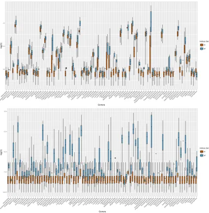
countsW. The top panel of Figure 2.1 shows the boxplots of the estimated compositionsXb except

common generaBacteroides, Blautiaand Roseburia that have been observed in all individuals.

Overall, we observed that the observed non-zero compositions had an effects in estimating the

compositions with zeros counts and the estimated compositions in those with zero observations

(M) were almost always smaller than those with non-zero observations (Mc_{). However, results}

from the simple zero replacement (Xbs) gave almost the same estimates for all samples/taxa inM.

The observed non-zero compositions almost had no effects in estimating the compositions with

−9 −6 −3 Abiotrophia Acetanaerobacter ium Acidaminococcus Akk

ermansiaAlistipes_Allisonella AnaerococcusAnaerofilumAnaerofustisAnaerostipes_Anaerotr

uncus

Anaero vorax

Asaccharobacter AtopobiumBacillusBarnesiella

Butyr icicoccus Butyr icimonas Camp ylobacter CapnocytophagaCatenibacter ium CloacibacillusClostr idium Collinsella

CoprobacillusCoprococcusDesulf ovibr io DialisterDorea Egger thella EnterococcusEubacter ium Faecalibacter ium Finegoldia Fusobacter ium Gemella

GordonibacterGran ulicatella HoldemaniaHow

ardella

LactobacillusLactococcusLactonif actor Leptotr ichia MegamonasMegasphaer a Meth ylobacter ium Mitsuok ella Mogibacter ium Neisser ia Odor ibacter Olsenella Oribacter ium OscillibacterOxalobacter ParabacteroidesPar

apre votella

ParasutterellaPar vimonas Peptoniphilus Peptostreptococcus Phascolarctobacter ium Porph yromonasPrevotella

Pseudob utyr

ivibr io

PseudomonasPyramidobacterRobinsoniellaRuminococcus_{Rummeliibacillus} Slackia Solobacter ium Sporobacter Stenotrophomonas Streptococcus Subdoligr anulum Succiniclasticum Succinivibr io

Sutterella_Turicibacter_VeillonellaVictiv allis

Weissella_Zymophilus

Genera log(X) Indices Set M Mc −10.0 −7.5 −5.0 −2.5 0.0 Abiotrophia Acetanaerobacter ium Acidaminococcus Akk

ermansiaAlistipes_Allisonella AnaerococcusAnaerofilumAnaerofustisAnaerostipesAnaerotr

uncus

Anaero vorax

Asaccharobacter AtopobiumBacillusBar

nesiella Butyr icicoccus Butyr icimonas Camp ylobacter CapnocytophagaCatenibacter ium CloacibacillusClostr idium Collinsella

CoprobacillusCoprococcusDesulf ovibr io DialisterDorea Egger thella EnterococcusEubacter ium Faecalibacter ium Finegoldia Fusobacter ium Gemella

GordonibacterGran ulicatella

HoldemaniaHow ardella

LactobacillusLactococcusLactonif actor Leptotr ichia MegamonasMegasphaer a Meth ylobacter ium Mitsuok ella Mogibacter ium Neisser ia Odor ibacter Olsenella Oribacter ium OscillibacterOxalobacter Par

abacteroides_Parapre votella

ParasutterellaPar vimonas Peptoniphilus Peptostreptococcus Phascolarctobacter ium Porph yromonasPre votella Pseudob utyr ivibr io

PseudomonasPyramidobacterRobinsoniellaRuminococcus Rummeliibacillus Slackia Solobacter ium Sporobacter Stenotrophomonas Streptococcus Subdoligr anulum Succiniclasticum Succinivibr io

Sutterella_Turicibacter_VeillonellaVictiv allis

Weissella_Zymophilus

Genera

log(X)

Indices Set

M Mc

Figure 1.7: Boxplots of the estimated compositions for each genus for those with zero observations (M) and those with non-zero observations (Mc_{). Top panel: proposed estimator}

b

X; Bottom panel: estimator with zero-replacementXbs.

1.7. Discussion

We have considered the problem of estimating the bacterial compositions based on sequencing

data, particularly for those taxa with zero observed counts, one of the first step in any microbiome

and metagenomic studies. We have developed a penalized likelihood estimation method for

utilizes data across different individuals and across different taxa, which is in contrast to most of

the available methods and has the flavor of shrinkage estimate. The estimation procedure makes

two key assumptions. First, it assume that the true microbial compositions are always positive and

the zero counts observed in metagenomic sequencing are due to under sampling. Our empirical

data (Figure 1.5) seems to support this assumption. Second, it assumes that the true composition

matrix has approximately low-rank structure. Under these assumptions, we have proposed a

pe-nalized likelihood estimation with a nuclear norm penalty function in order to obtain better estimate

of the composition matrix. We have obtained the estimation upper bounds and also the min-max

lower bounds and showed that our estimator is almost optimal. We have additionally obtained the

upper bounds for the estimates of various commonly used diversity indices, including Shannon’s

index, Simpson’s index and Brey-Curtis index. The resulting composition estimates can facilitate

other downstream compositional data analysis, such as high dimensional regression analysis (Lin

CHAPTER 2

L

C

E

C

D

C

-A

T

In this chapter, we address the problem of covariance estimation for high-dimensional

composition-al data, and introduce a composition-adjusted thresholding (COAT) method under the assumption

that the basis covariance matrix is sparse. Our method is based on a decomposition relating the

compositional covariance to the basis covariance, which is approximately identifiable as the

di-mensionality tends to infinity. The resulting procedure can be viewed as thresholding the sample

centered log-ratio covariance matrix and hence is scalable for large covariance matrices. We

rig-orously characterize the identifiability of the covariance parameters, derive rates of convergence

under the spectral norm, and provide theoretical guarantees on support recovery. Simulation

s-tudies demonstrate that the COAT estimator outperforms some naive thresholding estimators that

ignore the unique features of compositional data. We apply the proposed method to the analysis of

a microbiome dataset in order to understand the dependence structure among bacterial taxa in the

human gut.

2.1. Introduction

Compositional data, which represent the proportions or fractions of a whole, arise naturally in a

wide range of applications; examples include geochemical compositions of rocks, household

pat-terns of expenditures, species compositions of biological communities, and topic compositions of

documents, among many others. This article is particularly motivated by the metagenomic analysis

of microbiome data. The human microbiome is the totality of all microbes at various body sites,

whose importance in human health and disease has increasingly been recognized. Recent studies

have revealed that microbiome composition varies based on diet, health, and the environment (The

Human Microbiome Project Consortium, 2012a), and may play a key role in complex diseases such

as obesity, atherosclerosis, and Crohn’s disease (Koeth et al., 2013; Lewis et al., 2015; Turnbaugh

et al., 2009).

the microbiome composition using direct DNA sequencing of either marker genes or the whole

metagenomes. After aligning these sequence reads to the reference microbial genomes, one can

quantify the relative abundances of microbial taxa. These sequencing-based microbiome studies,

however, only provide a relative, rather than absolute, measure of the abundances of community

components. The counts comprising these data (e.g., 16S rRNA gene reads or shotgun

metage-nomic reads) are set by the amount of genetic material extracted from the community or the

se-quencing depth, and analysis typically begins by normalizing the observed data by the total number

of counts. The resulting fractions thus fall into a class of high-dimensional compositional data that

we focus in this article. The high dimensionality refers to the fact that the number of taxa may be

comparable to or much larger than the sample size.

An important question in metagenomic studies is to understand the co-occurrence and co-exclusion

relationship between microbial taxa, which would provide valuable insights into the complex ecology

of microbial communities (Faust et al., 2012). Standard correlation analysis from the raw

propor-tions, however, can lead to spurious results due to the unit-sum constraint; the proportions tend to

be correlated even if the absolute abundances are independent. Such undesired effects should be

removed in an analysis in order to make valid inferences about the underlying biological processes.

The compositional effects are further magnified by the low diversity of microbiome data, that is, a

few taxa make up the overwhelming majority of the microbiome (Friedman and Alm, 2012).

LetX= (X1, . . . , Xp)T be a composition ofpcomponents (taxa) satisfying the simplex constraint

Xj>0, j= 1, . . . , p, p

X

j=1

Xj = 1.

Owing to the difficulties arising from the simplex constraint, it has been a long-standing question

how to appropriately model, estimate, and interpret the covariance structure of compositional data.

The pioneering work of Aitchison, (1982, 2003) introduced several equivalent matrix specifications

of compositional covariance structures via the log-ratios of components. Statistical methods based

is crucial for our applications to microbiome data analysis.

Covariance matrix estimation is of fundamental importance in high-dimensional data analysis and

has attracted much recent interest. It is well known that the sample covariance matrix performs

poorly in high dimensions and regularization is thus indispensable. Bickel and Levina, (2008) and

El Karoui, (2008) introduced regularized estimators by hard thresholding for large covariance

ma-trices that satisfy certain notions of sparsity. Rothman, Levina, and Zhu, (2009) considered a more

general class of thresholding functions, and Cai and Liu, (2011) proposed adaptive thresholding

that adapts to the variability of individual entries. Exploiting a factor model structure, Fan, Fan,

and Lv, (2008) proposed a factor-based method for high-dimensional covariance matrix estimation.

Fan, Liao, and Mincheva, (2013) extended the work by considering a conditional sparsity structure

and developed a POET method by thresholding principal orthogonal complements.

In this article, we address the problem of covariance estimation for high-dimensional compositional

data. LetW= (W1, . . . , Wp)T withWj >0for alljbe a vector of latent variables, called thebasis,

that generate the observed data via the normalization

Xj =

Wj

Pp

i=1Wi

, j= 1, . . . , p. (2.1)

Estimating the covariance structure ofWhas traditionally been considered infeasible owing to the

apparent lack of identifiability. By exploring a decomposition relating the compositional covariance

to the basis covariance, we find, however, that the nonidentifiability vanishes asymptotically as

the dimensionality grows under certain sparsity assumptions. More specifically, define thebasis

covariance matrixΩ0= (ω0ij)p×p by

ω0_ij = Cov(Yi, Yj), (2.2)

whereYj = logWj. ThenΩ0is approximately identifiable as long as it belongs to a class of large

sparse covariance matrices.

The somewhat surprising “blessing of dimensionality” allows us to develop a simple, two-step

method by first extracting a rank-2 component from the decomposition and then estimating the

sparse component Ω0 by thresholding the residual matrix. The resulting procedure can

optimization-free and scalable for large covariance matrices. We call our method

composition-adjusted thresholding (COAT), which removes the “coat” of compositional effects from the

covari-ance structure. We derive rates of convergence under the spectral norm and provide theoretical

guarantees on support recovery. Simulation studies demonstrate that the COAT estimator

out-performs some naive thresholding estimators that ignore the unique features of compositional data.

We illustrate our method by analyzing a microbiome dataset in order to understand the dependence

structure among bacterial taxa in the human gut.

The covariance relationship, which was due to Aitchison, (2003 sec. 4.11), has recently been

ex-ploited to develop algorithms for inferring correlation networks from metagenomic data (Ban, An,

and Jiang, 2015; Fang et al., 2015; Friedman and Alm, 2012). Our contributions here are to turn

the idea into a principled approach to sparse covariance matrix estimation and provide statistical

insights into the issue of identifiability and the impacts of dimensionality. Our method also bears

some resemblance to the POET method proposed by Fan, Liao, and Mincheva, (2013) in that

un-derlying both methods is a low-rank plus sparse matrix decomposition. The rank-2 component

in our method, however, arises from the covariance structure of compositional data rather than a

factor model assumption. As a result, it can be obtained by simple algebraic operations without

computing the principal components.

The rest of the article is organized as follows. Section 2 reviews a covariance relationship and

addresses the issue of identifiability. Section 3 introduces the COAT methodology. Section 4

inves-tigates the theoretical properties of the COAT estimator in terms of convergence rates and support

recovery. Simulation studies and an application to human gut microbiome data are presented in

Sections 5 and 6, respectively. We conclude the article with some discussion in Section 7 and

relegate all proofs to the Appendix.

2.2. Identifiability of the Covariance Model

-In the latent variable covariance model (2.1) and (2.2), the basis covariance matrixΩ0is the

param-eter of interest. One of the matrix specifications of compositional covariance structures introduced

by Aitchison, (2003) is thevariation matrix T0= (τij0)p×p defined by

τ_ij0 = Var(log(Xi/Xj)). (2.3)

In view of the relationship (2.1), we can decomposeτ0

ijas

τ_ij0 = Var(logWi−logWj)

= Var(Yi) + Var(Yj)−2 Cov(Yi, Yj)

=ω0ii+ω

0

jj−2ω

0

ij, (2.4)

or in matrix form,

T0=ω01T+1ωT0 −2Ω0, (2.5)

whereω0 = (ω011, . . . , ωpp0 )T and 1= (1, . . . ,1)T. Corresponding to the many-to-one relationship

between bases and compositions, the basis covariance matrixΩ0 is unidentifiable from the

de-composition (2.5), since ω01T +1ωT0 and Ω0 are in general not orthogonal to each other (with

respect to the usual Euclidean inner product). In fact, using thecentered log-ratio covariance

ma-trix Γ0= (γij0)p×pdefined by

γ_ij0 = Cov{log(Xi/g(X)),log(Xj/g(X))},

whereg(x) = (Qp

j=1xj)1/p is the geometric mean of a vectorx = (x1, . . . , xp)T, we can similarly

write

τ_ij0 = Var{log(Xi/g(X))−log(Xj/g(X))}

= Var{log(Xi/g(X))}+ Var{log(Xj/g(X))} −2 Cov{log(Xi/g(X),log(Xj/g(X))}

=γ0_ii+γ_jj0 −2γ_ij0,

or in matrix form,

T0=γ01

T_+1γT

whereγ0 = (γ110 , . . . , γpp0 )T and1= (1, . . . ,1)T. Unlike (2.5), the following proposition shows that

(2.6) is an orthogonal decomposition and hence the componentsγ₀1T_+1γT

0 andΓ0are identifiable.

In addition, by comparing the decompositions (2.5) and (2.6), we can bound the difference between

Ω0and its identifiable counterpartΓ0as follows.

Proposition 3. The componentsγ₀1T_+1γT

0 andΓ0in the decomposition(2.6)are orthogonal to

each other. Moreover, for the covariance parametersΩ0andΓ0in the decompositions (2.5)and

(2.6),

kΩ0−Γ0kmax≤3p−1kΩ0k1.

Proposition 3 entails that the covariance parameter Ω0 is approximately identifiable as long as

kΩ0k1 = o(p). In particular, suppose that Ω0 belongs to a class of sparse covariance matrices

considered by Bickel and Levina, (2008),

U(q, s0(p), M)≡

 



Ω:Ω0,max

j ωjj ≤M,maxi p

X

j=1

|ωij|q≤s0(p)

 



, (2.7)

where0≤q <1andΩ0denotes thatΩis positive definite. Then

kΩ0k1= max

i p

X

j=1

|ω0_ij|1−q_|ω0

ij|

q _≤max i

p

X

j=1

(ω0_iiω_jj0)(1−q)/2|ω0_ij|q _≤M1−q_s

0(p),

and hence the parametersΩ0andΓ0are asymptotically indistinguishable whens0(p) =o(p). This

allows us to useΓ0as a proxy forΩ0and greatly facilitates the development of new methodology

and associated theory. The intuition behind the approximate identifiability under the sparsity

as-sumption is that the rank-2 componentω01T +1ωT0 represents a global effect that spreads across

all rows and columns, while the sparse componentΩ0represents a local effect that is confined to

individual entries.

Also of interest is theexactidentifiability ofΩ0overL0-balls, which has been studied by Fang et al.,