Identification of Cocoa Pods with Image Processing and Artificial Neural Networks

(1)

https://dx.doi.org/10.22161/ijaems.4.7.3 ISSN: 2454-1311

Identification of Cocoa Pods with Image

Processing and Artificial Neural Networks

Sergio A. Veites-Campos

1

_{, Reymundo Ramírez-Betancour}

2

_{, Manuel}

González-Pérez

3

1*_{Department of Mechatronic, M. Robotics, Universidad Autónoma de Guadalajara Campus Tabasco, Tabasco, México.}

2_{Faculty of Engineering and Architecture, Universidad Juárez Autónoma de Tabasco, Tabasco, México.} 3_{Universidad Popular Autónoma del Estado de Puebla, Puebla, México.}

*_{Corresponding author: Sergioveites@outlook .com}

Abstract— Cocoa pods harvest is a process where peasant mak es use of his experience to select the ripe fruit. During harvest, the color of the pods is a ripening indicator and is related to the quality of the cocoa bean. This paper proposes an algorithm capable of identifying ripe cocoa pods through the processing of images and artificial neural network s. The input image pass in a sequence of filters and morphological transformations to obtain the features of objects present in the image. From these features, the artificial neural network identifies ripe pods. The neural network is trained using the scaled conjugate gradient method. The proposed algorithm, developed in MATLAB ®, obtained a 91% of assertiveness in the identification of the pods. Features used to identify the pods were not affected by the capture distance of the image. The criterion for selecting pods can be modified to get similar samples with each other. For correct identification of the pods, it is necessary to tak e care of illumination and shadows in the images. In the same way, for accurate discrimination, the morphology of the pod was important.

Keywords— Cocoa pod, Processing of digital images, Artificial Neural Networks.

I. INTRODUCTION

Cocoa (Theobroma cacao L.) has been cultivated in America for thousands of years. Currently, all types of cultivated cocoa are varieties of numerous natural crosses or human intervention; however, is possible to classify the cocoa into three broad groups: Criollo or native, Forastero or peasant, Trinitario or hybrid [1,2].

The Cocoa Pod is an indehiscent berry. The pods’ size oscillates from 10 to 42 cm in variable form (oblong, elliptical, oval, spherical and oblate), the surface of the fruit can be smooth or rough, the colors of the surface can be red or green in the immature state [3]. Some authors consider that the shape of the pod is a reference point for classifying cultivated cocoa trees. The classifying of cocoa by its shape divides among Amelonado, Calabacillo, Angoleta, and Cundeamor [1,4]. A

significant determinant of pod ripening is the outward appearance. The ripening is visible as the colors of the pod´s external walls change. Usually, the outer walls turn green or purple changing to shades of red, orange or yellow depending on the genotype [5].

The ideal condition for pods harvest is when they are ripe. It is essential not to let the pods overripening as they can contaminate with some fungal diseases. The state of overripening promotes the germination of seeds and causes quality defects. Green fruits should not be part of the harvest. The seeds of green pods are hard, they cannot be separated easily and do not ferment because the mucilage is not finished forming [6].

For a proper fermentation, it is recommended to separate the pods according to their shape, color, and size to avoid the combination of seeds varieties. Ripeness degree of the pods determines the quality of cocoa bean s. No mixtures of pods with different ripen estate should be generated , mainly when it is sold to process fine chocolates. The main chocolate industries look for a unique origin and reject the mixtures of varieties [7].

In food, color is one of the factors considered by the customer at the moment of the purchase of a product. The color is a quality criterion in many classification standards. The color is a parameter used to evaluate the ripening status of fruits [8]. Thus, different technologies have been implemented to harvest fruits in their best conditions.

Artificial vision systems incorporate color information. Within the range of visible wavelengths, some compounds in fruits absorb the light. These compounds are pigments, such as chlorophylls, carotenoids, and anthocyanins [9].

(2)

ripening. The use of vision systems allows replacing the use of color charts, colorimeters and spectrophotometers [8]. Colorimeters has deficiencies to describe perceptual chromatic responses with a multitude of visual parameters [10].

Digital image processing involves methodologies for analyzing and finding quantitative information. The tools and algorithms for the capture of images allow evaluating in a non-destructive way [8]. Since a few years ago, these methodologies were applied. Some examples are listed below: Systems for recognition and localization of quasi-spherical objects by laser telemetry [11], processing of optical images of cherry coffee fruits by acoustic-optical filters [12], Systems to identify the color of the epicarp of tomatoes [13], a mobile platform for the collection of oranges [14], and analysis of fruits such as wheat, Feijoa, Mango, plantain and mandarins [15,16, 17,18].

On the other hand, the use of artificial neural networks (ANNs) and artificial vision has more application in the food industry recently. The ANNs prioritize the classification, the recognition of patterns and the prediction of crops [19]. ANNs try to emulate the behavior of the human brain. The ANNs extract knowledge from a set of data obtained during training. ANNs can be considered as models of calculation that uses very efficient algorithms, which operate in a massively parallel way. These artificial nets allow developing cognitive tasks like learning patterns, classification or optimization [20]. Most applications in ANNs are related to pattern recognition problems and make use of architectures such as multilayer perceptron [21].

The techniques of image processing and ANNs are applied as a methodology for classification of Royal Gala apples. In these techniques, a multilayered neural network was implemented through supervised learning and trained with different algorithms [22].

In this paper, we proposed the processing of images with artificial neuronal networks in the harvest of Cocoa pods using images taken by a photographic camera. Subsequently, from the objects contained in the image, it obtains a matrix of data. Finally, we process the data from the matrix using the data from previous training. This methodology improves the harvest process substituting the handcrafted way. With this methodology, the human perception of the color of the cocoa pod is removed and controls the quality of the harvested fruit.

II. PROCESSING ALGORITHM

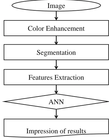
The proposed processing algorithm is divided into four steps (Fig. 1). The algorithm processes an image in JPEG format with dimensions of 1920 x 1080 pixels using the RGB color space (Red, Green, Blue). The image should have good saturation and the least ambient noises. First

three steps remove the colors that are not typical of the ripe cocoa pods and gets the features of the found objects. An ANN evaluates these features . Therefore, the result of the algorithm is the identifier of the ripe cocoa pods on the input image.

Fig. 1: Processing algorithm

2.1 Color Enhancement

The first step of the algorithm is to improve the colors of the input image. The lack of color intensity can be enhanced by adjusting the saturation values. For making it with less computational effort, it is proposed to convert the image in RGB color space to HSV (Hue, Saturation, Value). The three primary components that integrate the HSV color space are hue, saturation, and brightness [23]. The matrices of the HSV space has the same dimension as the RGB image. Assuming that values below 25% characterize obscure colors, the elements of the saturation matrix 𝑺 are modified by,

𝑠𝑖,𝑗 = {

0.8, 𝑠𝑖,𝑗 > 0.25

𝑠𝑖,𝑗, 𝑠𝑖,𝑗 ≤ 0.25

⋯ (1)

𝑠𝑖,𝑗 ⊂ 𝑺,

𝑺 ∈ ℳ𝑚𝑥𝑛(ℂ),

ℂ = {𝑥 ∈ ℝ , 0 ≤ 𝑥 ≤ 1}, 𝑅𝑜𝑤𝑠 𝑖, 1 ≤ 𝑖 ≤ 𝑚, 𝐶𝑜𝑙𝑢𝑚𝑛𝑠 𝑗, 1 ≤ 𝑗 ≤ 𝑛.

Consequently, the new saturation matrix holds the dark colors that could represent a flaw in the cocoa pods. To end this stage, the image in the HSV color space converts into the RGB color space. The conversion is done to avoid alterations in the properties of the colors during the following steps of the algorithm [23]. Figure 2 shows the performance of this stage of the algorithm.

Image

Color Enhancement

ANN

Features Extraction

(3)

(a) (b)

Fig. 2: (a) Original image, (b) Enhanced image

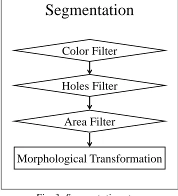
2.2 Segmentation

Before the extraction of features, in the segmentation stage of processing, the image is prepared first. Environmental noises and unwanted objects are filtered in the image to acquire reliable features (Fig. 3). At the end of this stage, is get a binary image with smoothed edges.

Fig. 3: Segmentation steps

2.2.1Color Filter

In this segmentation stage, the RGB image is processed to remove several colors ranges through five filters. The colors excluded are white, blue, magenta, green, brown, and some red hues. Relational operators and logical gates form the color filters . The result of the filters is a binary image.

The white filter creates a 𝑭1 matrix that meets the conditions of Equation 2. The blue tonalities generate a second 𝑭2 matrix that complies with Equation 3. Magenta colors and red hues provide a third 𝑭3 matrix that satisfies Equation 4. While the green color, is represented by the 𝑭4 matrix created by Equation 5. Finally, Equation 6 represents the filter of yellow colors, brown, and some orange shades. The conditions of the last filter create the

𝑭5 matrix. This final filter is calibrated according to the desired ripening of the cocoa pods.

𝑓1𝑖,𝑗 = (𝑟𝑖 ,𝑗≥ 235 ) &(𝑔𝑖,𝑗 ≥ 235) & (𝑏𝑖,𝑗≥ 235), ⋯ (2)

𝑓2𝑖,𝑗 = (𝑏𝑖,𝑗 ≥ 𝑔𝑖 ,𝑗) &(𝑏𝑖,𝑗 > 𝑟𝑖,𝑗), ⋯ (3)

𝑓3𝑖,𝑗 = (𝑟𝑖 ,𝑗≥ 𝑏𝑖,𝑗) &(𝑔𝑖,𝑗≤ 𝑏𝑖,𝑗) , ⋯ (4)

𝑓4𝑖,𝑗 = (𝑔𝑖 ,𝑗> 𝑟𝑖 ,𝑗) &(𝑔𝑖,𝑗 > 𝑏𝑖,𝑗), ⋯ (5)

𝑓5𝑖,𝑗 = ((|𝑔𝑖,𝑗− 𝑏𝑖,𝑗|) ≤ 𝑦) &((𝑟𝑖,𝑗 > 𝑔𝑖,𝑗)&(𝑟𝑖 ,𝑗> 𝑏𝑖,𝑗)),

⋯ (6) 𝑟𝑖,𝑗 ⊂ 𝑹 , 𝑔𝑖,𝑗 ⊂ 𝑮 , 𝑏𝑖,𝑗 ⊂ 𝑩 ,

𝑓1𝑖,𝑗 ⊂ 𝑭1 , 𝑓2𝑖,𝑗 ⊂ 𝑭2 , 𝑓3𝑖,𝑗 ⊂ 𝑭3 ,

𝑓4𝑖,𝑗 ⊂ 𝑭4 , 𝑓5_𝑖,𝑗 ⊂ 𝑭5 ,

[𝑅 , 𝐺 , 𝐵] ∈ ℳ𝑚𝑥𝑛(𝔻) ,

𝔻 = {𝑥 ∈ ℕ , 0 ≤ 𝑥 ≤ 255}, [𝐹1, 𝐹2 , 𝐹3, 𝐹4, 𝐹5] ∈ ℳ𝑚𝑥𝑛(𝕂),

𝕂 = {0,1},

𝑦 ∈ ℕ , 0 ≤ 𝑦 ≤ 255 , 𝑅𝑜𝑤𝑠 𝑖, 1 ≤ 𝑖 ≤ 𝑚, 𝐶𝑜𝑙𝑢𝑚𝑛𝑠 𝑗, 1 ≤ 𝑗 ≤ 𝑛,

where 𝑹, 𝑮, and 𝑩 represent the RGB matrix color space and, 𝑦 represents the filter five setting to calibrate the color hue.

The resulting matrix of filters is added to obtain a matrix containing all the excluded tonalities,

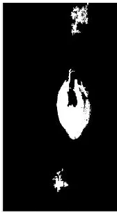
𝑭𝑭 = 𝑭1 + 𝑭2 + 𝑭3 + 𝑭4 + 𝑭5. ⋯ (7) Therefore, the logical negation of 𝑭𝑭 provides the binary image with the required tonalities. Color filtering can be seen in Figure 4

Fig. 4: Filtered and binarized image

2.2.2Holes Filter

The second segmentation stage removes the holes of the objects found in the binary image. It is proposed to eliminate these holes to improve the results in the morphology stage. Not all holes are covered. Those small holes resulting from reflections on the objects are filled in. Large holes generated by dark spots are not eliminated. Naturally the pods have small dark marks; however, large spots on a cocoa pod are a quality defect.

Color Filter

Area Filter

Morphological Transformation

Holes Filter

Segmentation

(4)

Identifying the holes consists of finding all the values of 0 in the 𝑬1 matrix that are isolated from the values that make up the background of the binary image. The largest neighborhood group of elements in the 𝑬1 matrix with a value of 0 form the background of the image. Isolated elements are called holes. For identify holes, the "imfill" function of MATLAB ® is applied. The function produces a binary matrix 𝑯, which contains the holes founded in the input image and represents them with a value of 1 [24].

From 𝑯, an 𝑯1 matrix containing holes formed by light reflections is obtained,

𝑯1 = 𝑯 & 𝑭1, ⋯ (9)

[𝑯, 𝑯1] ∈ ℳ𝑚𝑥𝑛(𝕂).

Also, using the methodology described in the following section (Area Filter) the 𝑯2 matrix is generated. This matrix represents the smaller holes. The matrices obtained are added, and a matrix is gotten with the holes to be filled,

𝑯𝐹 = 𝑯1 +

𝑯2. ⋯ (10)

Finally, the holes in the original image are filled through

𝑬2 = 𝑬1 + 𝑯𝑭, ⋯ (11)

where 𝑬2 represents an image without holes. In Figure 5, the application of the Hole Filter stage can be seen in Figure 4.

Fig. 5: Filtered image without holes 2.2.3Area Filter

There are small objects in the binary image gotten in the previous step. Small groups of pixels and isolated pixels with a value of 1, shape these objects. Removing these pixels from the background of the image makes hold large objects. The third stage of the segmentation, filter the objects by their areas. The methodology removes all neighborhood groups of elements with a value of 1 in the 𝑬2 matrix. For this, the areas of the neighborhood groups are analyzed in the matrix. Using the "Blob Analysis" function of SIMULINK ® is possible to get areas [24]. From this function is obtained the data of the areas and a

matrix of Bounding boxes. With the areas of the neighborhood groups found is created a vector column 𝑨.

The matrix of 𝑩𝑩 contains the coordinates and size of Bounding Boxes. These enclose the neighborhood groups found in the input matrix entered into the function. In base on vector 𝑨, is created a reference vector 𝑸,

𝑞𝑘,1 = (𝑎𝑘,1 < 𝑥), ⋯ (12)

𝑞𝑘,1 ⊂ 𝑸 , 𝑎𝑘,1 ⊂ 𝑨,

𝑨 ∈ ℳ𝑚𝑥1(ℝ+),

𝑸 ∈ ℳ𝑚𝑥1(𝕂),

𝑅𝑜𝑤𝑠 𝑘, 1 ≤ 𝑘 ≤ 𝑧,

where 𝑥 is the minimum allowed area and 𝑧 is the number of neighborhood groups found in the 𝑬2 matrix.

With the values of 𝑸, a reference matrix 𝑾𝑾 is generated, which is created from the horizontal concatenation of 𝑸 with itself four times. The above is done to equal the dimensions of 𝑸 and 𝑩𝑩. Based on 𝑾𝑾 the elements of 𝑩𝑩 are conditioned,

𝑏𝑏𝑘,4= {

𝑏𝑏𝑘,4 , 𝑤𝑤𝑘,4= 1

0, 𝑤𝑤𝑘,4= 0

⋯ (13)

𝑏𝑏𝑘,4 ⊂ 𝑩𝑩 , 𝑤𝑤𝑘 ,4

⊂ 𝑾𝑾 ,

𝑩𝑩 ∈ ℳ𝑚𝑥4(ℝ),

𝑾 ∈ ℳ𝑚𝑥4(𝕂),

𝑅𝑜𝑤𝑠 𝑘, 1 ≤ 𝑘 ≤ 𝑧.

Finally, over the elements of 𝑬2 is drawn with 0 Bounding Boxes of 𝑩𝑩. The matrix obtained from this procedure is called 𝑬3 and characterizes the binary image filtered by area. This way, smaller objects are removed, and a cleaner image is obtained. Figure 6 shows the performance of this stage.

Fig. 6: Image filtered by area 2.2.4Morphological Transformation

(5)

perimeter. The modifications do not generate change in the dimension of the binary image.

The first part of the transformation is to apply a dilatation followed by erosion to 𝑬3. This technique is known as a closing function, and its output is a new binary matrix. This function eliminates small apertures at the edges of objects. Then, an erosion is applied followed by a dilation. This last technique is known as opening and creates the resulting matrix 𝑬4. With the opening function, is possible to remove small groups of pixels in the reliefs of the objects [25]. For the transformations mentioned above, the radius of the structuring element in the closing function must be less than the opening function. In Figure 7 the changes are appreciated comparing with Figure 6.

Fig. 7: Image with morphological transformation

2.3 Features Extraction

This stage gets the features of the object in the image.

These features are used to discriminate objects, which do not have the shapes of cocoa pods. Using "Blob Analysis" from SIMULINK ® are gotten these features and the matrix of Bounding Boxes [24]. The features obtained for this processing were: major axis, minor axis, eccentricity, and extent. The extent feature represents a relationship between the area of the found object and the area of its Bounding Box [26]. Features extracted are in the form of column vectors. Features of the major axis and minor axis are joined to represent the following relation:

𝑼 =

⌊ 𝑂1,1

𝑣1,1

𝑂2,1

𝑣2,1

⋮ 𝑂𝑘,1

𝑣𝑘,1⌋

⋯ (14)

𝑜𝑘 ,1 ⊂ 𝑶 , 𝑣𝑘,1 ⊂ 𝑽,

𝑽 ∈ ℳ𝑚𝑥1( ℝ+),

𝑶 ∈ ℳ𝑚𝑥1( ℝ+),

𝑼 ∈ ℳ𝑚𝑥1( ℂ),

𝑅𝑜𝑤𝑠 𝑘, 1 ≤ 𝑘 ≤ 𝑧1,

where 𝑼 represent the result of dividing the axis vectors, 𝑶 the minor axis, 𝑽 major axis, and 𝑧1 the number of

objects in the 𝑬4 image.

There are two significant advantages of the features obtained at this stage. The first is the performance of the three features (relation of axes, eccentricity, and extent) over ovoid objects. Finally, the value of the features tends to be retained with the distance; as shown in Figure 8.

(a)

(b)

Fig. 8: (a) Pod about a meter away, (b) Pod two meters away.

Finally, in this stage is generated the matrix of 𝑩𝑭 Bounding Boxes that enclose the found objects and the matrix 𝑪 that contains the features of the objects. Matrix 𝑪 come from the horizontal concatenation of the three vectors containing the features separately.

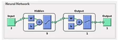
2.4 Artificial Neuronal Network (ANN)

In this last stage, the ANN received the features gotten in the previous step. Each feature creates inputs to the Artificial Neuronal Network and, the output relates the inputs by functions [27]. Therefore, the network will be made up of three inputs and a single output. The output is a Real number between 0 and 1. The approximation of the output to 1 indicates that the values of the features come from a cocoa pod.

Within the three fundamental operations of the artificial neuron, the transfer function 𝑓 is related to the type of output (Fig. 9). From the existing transfer functions, the sigmoidal function is selected for this application. This function takes inputs between negative infinity and positive infinity. The output of the sigmoidal function generate values between 0 and 1 [27].

Eccentricity

Extent

0.784 0.620 0.767

Eccentricity

Extent

(6)

Fig. 9: Single input neuron [27]

The output of a simple artificial neuron with sigmoidal transfer function is described by,

𝑡 = 𝑙𝑜𝑔𝑠𝑖𝑔 (𝑤𝑝 + 𝑏), ⋯ (15) [𝑤, 𝑝, 𝑏] ∈ ℝ,

𝑡 ∈ ℂ,

where 𝑡 is the network output, 𝑝 is the input variable to the neuron, 𝑤 is the net weight and 𝑏 is the bias.

A single-layer ANN is deficient for this processing algorithm. Therefore, a multi-layered ANN has been designed. The type of ANN proposed here will be a Feedforward Neuronal Network (FNN). This type of networks behaves with good results in pattern recognition and object classification applications. The number of layers used in this work is two, as recommended by [27]. Finally, the designed network has nine neurons in its first layer and a single neuron in the output layer (Fig. 10).

Fig. 10: Feedforward Neuronal Network

Feedforward Neuronal Network can use the scaled conjugate gradient method for training. For large networks, this training algorithm is the most efficient. The pattern recognition problems frequently apply this method [27].

The methodology of the FNN designed is to read the data of 𝑪. Each row contains the features of an individual object. The single output of the network will be based mainly on the features extracted and weights of the FNN. The result of the network will be a scalar between 0 and 1. This value is conditioned by,

𝑡1 = 𝑡 ≥ 𝑙 , ⋯ (16)

𝑡 ∈ ℂ,

𝑙 ∈ ℂ, 𝑡1 ∈ 𝕂,

where 𝑡 is the output of the FNN, 𝑡1 is the conditioned

output and 𝑙 is the criterion that conditions the output. This criterion is in function of the percentage of the output coincidence with the samples in the training.

With the values of 𝑡1 is created the reference column

vector 𝑸1. This vector comes from the vertical concatenation of the outputs of the FNN.

Based on 𝑸1, the 𝑾𝑭 matrix is generated, whose values are gotten from the horizontal concatenation of 𝑸1 with itself four times. The above is done to equal the dimensions of 𝑸1 and 𝑩𝑭. Then, the elements of 𝑩𝑭 are conditioned in the following way,

𝑏𝑓𝑘 ,4= {

𝑏𝑓𝑘 ,4 , 𝑤𝑓𝑘 ,4= 1

0, 𝑤𝑓𝑘 ,4= 0

⋯ (17)

𝑏𝑓𝑘 ,4 ⊂ 𝐵𝑭 , 𝑤𝑓𝑘 ,4 ⊂ 𝑾𝑭 ,

𝑩𝑭 ∈ ℳ𝑚𝑥4( ℝ),

𝑾 ∈ ℳ𝑚𝑥4( 𝕂),

𝑅𝑜𝑤𝑠 𝑘, 1 ≤ 𝑘 ≤ 𝑧1.

Finally, the image processing algorithm takes the 𝑩𝑭 data to draw the Bounding Boxes that point out to the cocoa pods on the RGB input image that this algorithm received. Using the SIMULINK ® "Draw Shapes" block, draw the Bounding Boxes over the RGB image.

III. RESULTS ANDDISCUSSION

The methodology proposed in this research was developed in MATLAB ® R2018A using the Visual Programming Environment SIMULINK ®. The simulation was done on a computer with Microsoft ® Windows ® 7 Home Premium, Intel ® Core ™ i7-2630QM 2.00 GHz processor and 8 Gb DDR3 1333Mhz RAM.

The images used for the development of the investigation were obtained from cacao farms of the village Cucuyulapa. This locality is part of the municipality of Cunduacán, Tabasco, Mexico. In the locality, images were taken with the natural daylight of midday. All the images taken had the same illumination and focal aperture. The images capture was taken at distances between 1 and 2 meters.

The types of pods used in this experiment were hybrids of

criollo cocoa with an amelonada shape. The observed color changes in these pods were from green to yellow. Some variations in the length of the pod were observed in the same cocoa genotype.

(7)

Table 1: Training results Cross-Entropy Percent Error Training 5.77386e-1 6.50406e-0 Validation 9.35257e-1 0

Testing 9.95469e-1 0

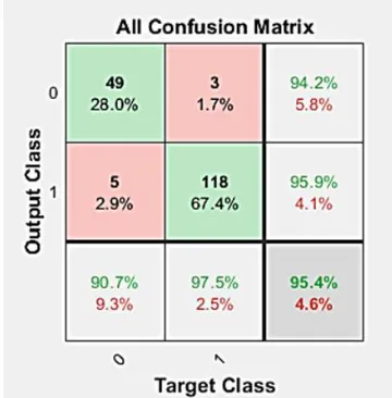
The identification of the objects leads us to create a confusion matrix. This matrix has the erroneous or successful percentages of the FNN to obtain its targets. Figure 11 represents the total confusion matrix of the training algorithm processes. The percentage of total assertiveness towards to the wanted Targets is 95.4%.

Fig. 11: All confusion matrix from FNN

The processing algorithm was tested using 23 images of cocoa pods different from those used in the training algorithm. The tests are in charge of evaluating the performance of the algorithm for each image at different values of the 𝑙 match criterion (Equation 16). Value of 𝑙

evaluates the image more stringent. A high value in 𝑙

allows making a homogeneous selection of pods in good shape and with proper ripening. According to the ripening of the pods, Table 2 shows the most appropriate values of

𝑙 for the algorithm.

Table 2: Test results

𝑙 Percent Assertiveness

0.7 89%

0.8 91%

0.9 91%

0.95 83%

The values of 𝑙 between 0.8 and 0.9 gets the best performance of the algorithm. Criterion of 0.95 presents a lower percentage of assertiveness because it penalizes the shape of the pod. The criterion of 0.95 is suitable if it is looking for pods that have the proper ripening and the average shape that characterizes the selected cocoa genotype. Finally, the criterion of 0.7 shows good results

to select ripe cocoa pods, but with the disadvantage of confusing some pods with some green hue. Then, in Figure 12, the result of the algorithm can be seen using 0.9 as the criterion for evaluating the sample.

(a) (b)

Fig. 12: (a) Image inputted, (b) Image result

The errors generated in the tests came from the values of the features in the pods. These values are affected by the length of long pods and pods with green color or spots at its ends. At the time of evaluating the features of these types of pods with considerable deviations in their form, the algorithm can recognize the samples as morphologically correct pods.

IV. CONCLUSION

In this work, a methodology was proposed to identify ripe criollo cocoa pods type amelonado. It could be observed that these fruits tend to change from green to yellow. The overripening make color changes on the pod to yellow to orange hues. Therefore, it was proposed to use a filter in which the desired tonality of the fruit could be adjusted. Also, the measurements of the features of the pods were essential to identifying if the pod presents damage for some disease.

The images taken for this algorithm were carried out taking care of lighting and light reflections. These factors cause noises that impair the calibration of the camera's colors and the adjustment of the desired hue of a pod. The modification of the saturation of the image helped to improve noises that derive from these factors; however, excessive shadows and reflections cause problems in digital image processing.

The use of the area filter helps the shapes in the images do not have so many morphological changes and to be able to eliminate objects that cause noises in the binary image. The previous methodology proposes to maintain as much as possible the original size of the forms and despite this eliminate noises by a group of pixels.

(8)

shapes. It could be seen that the features retained their value, regardless of the distance of the photograph. The performance of features represents an advantage, allowing selecting similar shapes without the need for a reference distance.

The technique of modifying the criterion of selection of samples in the processing algorithm behaved in the manner expected. In this way, it is possible to adjust the criterion making it more critical and having homogeneous samples. Getting good results within 80% and 90% of coincidence criterion with training samples. If the study objects have many variations in their shape, setting the selection criterion may not be the most appropriate. It is expected in future work to study the variations of pods of different genotypes. This study could select ripe cocoa pods from all types of shapes. The selection of these pods could be made without being confused with other objects. In the same way, the features should be improved or complemented, to avoid confusion between ripe pods and pods with possible morphological diseases.

REFERENCES

[1] Reyes Vayssade, M. (1992). Cacao: Historia, Economía y Cultura.Mexico City: Nestlé

[2] CacaoMexico.org (2010). Cacao México. Retrieved from https://www.cacaomexico.org/

[3] Avendaño, C. H., Villarreal, J. M., Campos, E.,

Gallardo, R.A, Mendoza, A., Aguirre, J. F., …

Zaragoza, S. E. (2011). Diagnóstico del cacao en México. Mexico City: Universidad Autónoma Chapingo.

[4] Lépido Batista. (2009). Morfología de la planta de

cacao. Retrieved from

http://www.fundesyram.info/biblioteca.php?id=3096

[5] Afoakwa, E. O. (2016). Chocolate science and technology. Oxford: John Wiley & Sons.

[6] Cubillos, G., Merizalde, G., & Correa, E. (2008).

Manual de beneficio del cacao. Antioquia: Secretaria de Agricultura de Antioquia.

[7] Lutheran Word Relief (2013). Cosecha, Fermentación y Secado del cacao (Guía 8). Retrieved from

http://cacaomovil.com/

[8] Padrón, C. A., León, M. G., Montes, A. I., & Oropeza, R. A. (2016). Procesamiento Digital de Imágenes: Determinación del color en muestras de alimentos y durante la maduración de frutos. Retrieved from

https://www.amazon.com/dp/B01MU1KOOF/ref=rdr _kindle_ext_tmb

[9] Viñas, M. I., Usall, J., Echeverria, G., Graell, J., Lara, I., & Recasens, D. I. (2013). Poscosecha de pera, manzana y melocotón. Madrid: Mundi-Prensa Libros. [10] Martínez Verdú, F. M. (2001). Diseño de un colorímetro triestímulo a partir de una cámara CCD-RGB. (Doctoral Thesis). Universidad Politécnica de

Catalunya, Department of Optica and Optometry, Barcelona. Retrieved from

http://hdl.handle.net/2117/94055

[11] Ruiz, A. R. J. (1998). Sistema de reconocimiento y localización de objetos cuasi-esféricos por telemetría láser. Aplicación a la detección automática de frutos para robot Agribot. (Doctoral Thesis). Universidad Complutense de Madrid,

Department of computer architecture and Automation,

Madrid.

[12] Mosquera, J. C., Sepúlveda, A., & Isaza, C. A. (2007). Procesamiento de imágenes ópticas de frutos café en cereza por medio de filtros acusto-ópticos. Ingeniería y Desarrollo, (21), 93-102. [13] Padrón Pereira, C. A., León, P., Marié, G., Montes

Hernández, A. I., & Oropeza González, R. A. (2012). Determinación del color en epicarpio de tomates (Lycopersicum esculentum Mill.) con sistema de visión computarizada durante la maduración. Agronomía Costarricense, 36(1), 97-111. [14] Tovar Yate, C. G. (2014). Desarrollo e

implementación de una plataforma móvil para recolección de naranjas. (Bachelor's Thesis). Universidad Católica de Colombia, Faculty of Engineering, Colombia.

[15] Acosta, C. P. S., Mir, H. E. V., García, G. A. L., Ruvalcaba, L. P., Hernández, V. A. G., & Olivas, A. R. (2017). Tamaño y número de granos de trigo

analizados mediante procesamiento de imagen digital. Revista Mexicana de Ciencias Agrícolas, 8(3), 517-529.

[16] Bonilla-González, J. P., & Prieto-Ortiz, F. A. (2016). Determinación del estado de maduración de frutos de feijoa mediante un sistema de visión por computador utilizando información de color. Revista de Investigación, Desarrollo e Innovación, 7(1), 111-126. doi: 10.19053/20278306.v 7.n1.2016.5603

[17] Alberto, C., Pereira, P., León, P., & Valencia, M. (2012). Determinación del color en epicarpios de mango (Mangifera sp.) y plátano (Musa AAB) en maduración mediante sistema de visión computarizada. Revista Venezolana de Ciencia y Tecnología de Alimentos, 3(2), 302-318.

[18] Padrón-Pereira, C. A. (2013). Utilización de imágenes digitales para medición del diámetro de frutos de mandarina (citrus reticulata) en crecimiento / Using digital images for measurement of mandarin (Citrus reticulata) Fruits Diameter During Growth. Ciencia y Tecnología, 6(1), 1-9.

(9)

[20] López, R. F., & Fernández, J. M. F. (2008). Las redes neuronales artificiales. La Coruña: Netbiblo. [21] Bishop, C., & Bishop, C. M. (1995). Neural

network s for pattern recognition. New York: Oxford University Press.

[22] Avila, G. A. F. (2016). Clasificación de la manzana royal gala usando visión artificial y redes neuronales artificiales. Research in Computing Science, 114, 23-32.

[23] Gil, P., Torres, F., & Ortiz Zamora, F. G. (2004).

Detección de objetos por segmentación multinivel combinada de espacios de color. Universidad de Alicate, Department of Physics, Systems Engineering

and Signal Theory, Alicate. Retrieved from

http://hdl.handle.net/10045/2179

[24] Matlab, Mathworks (2018). Image processing

Toolbox™ User's Guide. Retrieved from

https://la.mathworks.com/help/pdf_doc/images/index. html

[25] Ortiz Zamora, F. G. (2002). Procesamiento morfológico de imágenes en color: aplicación a la reconstrucción geodésica. (Doctoral Thesis). Universidad de Alicate, Department of Physics, Systems Engineering and Signal Theory, Alicate. Retrieved from http://hdl.handle.net/10045/10053

[26] Matlab, Mathworks (2018). Computer Vision System

Toolbox™ User's Guide. Retrieved from

https://la.mathworks.com/help/pdf_doc/vision/index.h tml