29
Software Defect Prediction using Adaptive Neural
Networks
Seema Singh
Lecturer in IT Department Lovely Professional University
H. no. 290, Village – Dhina P.O. Jalandhar cantt Punjab
Mandeep Singh
Lecturer in Management department Lovely Professional University H. no. 16, Police Station MullanpurDakha
Ludhiana Pin - 141101
ABSTRACT
We present a system which gives prior idea about the defective module. The task is accomplished using Adaptive Resonance Neural Network (ARNN), a special case of unsupervised learning. A vigilance parameter (θ) in ARNN defines the stopping criterion and hence helps in manipulating the accuracy of the trained network. To demonstrate the usefulness of ARNN, we used dataset from promisedata.org. This dataset contains 121 modules out of which 112 are not defected and 9 are defected. In this dataset modules are termed as defected on the basis of three measures that are LOC, HALSTEAD, MCCABE measures that have been normalized in the range of 0-1.We see that at θ=0.1858 the network has maximum Recall (i.e. true negative rate) is 100% and average Precision=54%.In case of ART n/w shortfalls are seen for Accuracy as this is a subjective measure.
Keyword:
Resonance, Clustering, Unsupervised learning, Confusion metrics.1. INTRODUCTION
Today software is used in almost every walk of life. The software development companies cannot risk their business by shipping poor quality software as it results in customer dissatisfaction. Risk to business can be minimized by predicting the quality of the software in the early stages of the software development lifecycle (SDLC). This would not only keep the clients satisfied but also reduce the cost of correction of defects. It has been reported in that the cost of detect correction is significantly high if the corrections are made after testing. An additional benefit of early prediction of software quality is better resource planning and test planning. Therefore the key is to identify defect prone modules at an early SDLC stage. The importance of early software quality prediction is evident from a number of studies conducted in the regard.
It is beneficial to obtain early estimates of system reliability or fault-proneness to help inform decisions on testing, code inspections, design rework, as well as financial costs associated with a delayed release, etc. In industry, estimates of system reliability (or pre-release defect density) are often available too late to affordably guide corrective actions to the quality of the software. Several studies have been performed to build models that predict system reliability and fault-proneness. Quality is considered a key issue in any software development project. However, many projects face a tradeoff between cost and quality, as the time and effort for applying software quality assurance measures is usually limited due to economic constraints. In practice, quality managers and testers are in a daily struggle with critical bugs and shrinking budgets.
Hence, they are eagerly looking for ways to make quality assurance and testing more effective and efficient. Defect prediction promises to indicate defect-prone modules in an upcoming version of software system and thus allows focusing the effort on those modules. The net result should be systems that are of higher quality, containing fewer faults, and projects that stay more closely on schedule than would otherwise be possible.
With real-time systems becoming more complex and unpredictable, partly due to increasingly sophisticated requirements, traditional software development techniques might face difficulties in satisfying these requirements. Further real-time software systems may need to dynamically adapt themselves based on the runtime mission-specific requirements and operating conditions. This involves dynamic code synthesis that generates modules to provide the functionality required to perform the desired operations in real-time. Telecontrol/telepresence, robotics, and mission planning systems are some of the examples that fall in this category. However, the necessitates the need to develop a real-time assessment technique that classifies these dynamically generated systems as being faulty/fault-free. Some of the benefits of dynamic dependability assessment include providing feedback to the operator to modify the mission objectives if the dependability is low, the possibility of masking defects at run-time, and the possibility of pro-active dependability management. One approach in achieving this is to use software defect prediction techniques that can assess the dependability of these systems using defect metrics that can be dynamically measured.
A variety of software defect prediction techniques have been proposed, but none has proven to be consistently accurate. These techniques include statistical methods, machine learning methods, parametric models and machine learning methods, parametric models, and mixed algorithms. Obviously, there is need to find the best prediction techniques for a given prediction technique for a given prediction problem in context, and perhaps, conclude that this problem is largely unsolvable.
2. WHAT IS A NEURAL NETWORK?
30 graph is a “labeled graph” if each connection is associated
with a label to identify some property of the connection. In a neural network, each node performs some simple computations, each connection conveys a signal from one node to another, labeled by a number called the “connection strength” or “weight” indicating the extent to which a signal is amplified or diminished by a connection. The roots of all work on neural networks are in century-old neuro-biological studies. The following century-old statement by William James (1890) is particularly insightful, and ids reflected in the subsequent work of many researchers. The amount of activity at any given point in the brain cortex is the sum of the tendencies of all other points to discharge into it, such tendencies being proportionate
1. To the number of times the excitement of other points may have accompanied that of the points in questions;
2. To the intensities of such excitements; and 3. To the absence of any rival point functionality
disconnected with the first point, into which the dischargers may diverted.
Most neural network learning rules have their roots in statistical correlation analysis and in gradient descent search procedures. Hebb‟s (1949) learning rule incrementally modifies connection weights by examining whether two connected nodes are simultaneously ON or OFF. Such a rule is widely used, with some modifications.
3. UNSUPERVISED LEARNING
Our neural network is based on unsupervised learning. A three-month-old child receives the same visual stimuli as a newborn infant, but can make much more sense of them, and can recognize various patterns and features of visual input data. These abilities are not acquired from an external teacher, and illustrate that a significant amount of learning is accomplished by biological processes that proceed “unsupervised” (teacher-less). Motivated by these biological facts, the artificial neural networks attempt to discover special features and patterns from available data without using external help.
Some problems require an algorithm to cluster or to partition a given data set into disjoint subsets (“clusters”), such that patterns in the same cluster are as alike as possible, and patterns in different clusters are as dissimilar as possible. The application of a clustering procedure results in a partition (function) that assigns each data point to a unique cluster. A partition may be evaluated by measuring the average squared distance between each input pattern and the centroid of the cluster in which it is placed.
4. ADAPTIVE RESONANCE THEORY
Adaptive resonance theory (ART) models are a neural network that performs clustering, and can allow the number of clusters to vary with the size of the problem. The major diffe3rences between ART and other clustering methods is that ART allows the user to control the degree of similarity between members of the same cluster by means of a user-defined constant called the vigilance parameter. It uses a MAXNET. A “maxnet” is a recurrent one-layer network that conducts a competition to determine which node has the highest initial input value. Apart from neural plausibility and the desire to perform every task using neural networks, it can be argued that the maxnet allows for greater parallelism in execution than the algebraic solution.
4.1 Proposed work
We presented a system to detect that whether a module is defected or not defected. Neural networks are used to perform this task. Most fault prediction techniques rely on historical data. Experiments suggest that a module currently under development is fault-prone if it has the same or similar properties, measured by software metrics, as a faulty module that has been developed or released earlier in the same environment. Therefore, historical information helps us to predict fault-proneness. Many modeling techniques have been proposed for and applied to software quality prediction. In neural networks historical data which is obtained by regression analysis or by any other means are fed to network and the network gets trained accordingly. That data is called training data. When we input operational data then network respond accordingly the trained data. So we used Adaptive Resonance Neural Networks (ARNN) which clusters already known modules which are faulty and fault-free. As it works under unsupervised learning so there is no distinction between training data and operational data.
We used data from promise data repository titled as „software defect prediction‟ which contains static attributes of some module codes. On the basis of these static attributes modules are termed as defected of defect-free. This module level static code attributes are collected using Prest metrics and analysis tool. The ARNN classifies the modules which are defected in one cluster and defect-free in another cluster.
5. RELATED WORK
Fault proneness is defined as the probability of the presence of faults in the software. Research on fault-proneness has focused on two areas:-the definition of metrics to capture software complexity and testing thoroughness and the identification of and experimentation with models that relate software metrics to fault-proneness. Fault-proneness can be estimated based on directly-measurable software attributes if associations can be established between these attributes and the system fault-proneness. Faults appear when a program does not perform according to user‟s specification during testing and operations stages. A number of techniques have been used for the analysis of software defect prediction. For example, optimized set reduction (OSR) techniques and logistic regression techniques are used for modeling risk and fault data. OSR attempts to determine which subset of observation from historical data provides the best characterization of the programs being assessed.
Munson et al. used discriminant analysis for classifying programs as fault-prone within a large medical-imaging software system. In their analysis, they also employed the data-splitting technique, where subset of programs are selected at random and used to train or build a model. The remaining programs are used to quantify the error in estimation of the number of faults.
5.1 Goal of defect prediction
31 group have worked on this prediction research. Our research
is focused on first type of goal.
5.2 Metrics for fault prediction
Many measures for fault prediction have been proposed in literature. They mainly capture the quality of Object-Oriented (OO) code and design for detecting fault proneness of modules. Mie Mie and Tong Seng [3] used the object oriented metrics for fault prediction to obtain assurance about software quality.
We can use software size and complexity metrics for predicting the number of defects in the system [9] or we can infer number of defects from testing information. It has also been observed that code change history is closely related to the number of faults that appear in modules of code [10]. Many of the metrics used for software defect prediction are highly correlated with lines of code, so when changes in code occurs the number of defects in module may change.
The study on the relationships between existing object-oriented coupling, cohesion and, inheritance measures and the probability of fault detection in system during testing has been performed by Briand et al.(2000). Their analysis has shown that many coupling and inheritance measures are strongly related to the probability of fault detection in a module. Their analysis has shown that by using some of the coupling and inheritance measures, very accurate models could be derived to predict in which classes most of the faults actually lie. Lots of factor affects software defect prediction, resulting in inconsistencies among learning methods. Hence, there is a need to develop methods that could remove some of the randomness (complexity/uncertainties) in the data leading us to a more definitive explanation of the error analysis. One of the steps is to capture the dependency among attributes using probabilistic models, rather than just using the “size” and “complexity” metrics. Bayesian belief networks (BBN) is one of the approach along this direction. Ourdataset used lines of code, Halsted and McCabe measures to find defects in the modules.
6.DESIGN, INPUT/OUTPUT AND
ALGORITHMS
This includes the dataset information, neural network used
and graphical user interface.
6.1 Dataset
The dataset used is a PROMISE Software Engineering Repository data set made publicly available in order to encourage repeatable, refutable, verifiable, and/or improvable predictive models of software engineering. The AR1 data is obtained from a Turkish white-goods manufacturer and it is denoted by Software research laboratory (softlab), Bogazici university, Istanbul, Turkey. It is a Prest Metrics Extraction and Analysis Tool, available at http://softlab.boun.edu.tr. It is embedded software in a white-goods product implemented in C. The dataset originally has 121 instances each with 30 parameters, having 9 are defective and 112 are defect-free. Each instance represents a software class (or module). A classification parameter is used as output to indicate if the software class is defect prone (D) or not-defect prone (ND). The rest of 29 static code parameters are software metrics. These complexity and size metrics include well known Line of Code (LOC) measures, Halstead and McCabe measures
calculated for that module and are divided into three groups. Group A has 5 parameters, Group B has 12 parameters and Group C has 12 parameters. The software metrics used in our dataset are described as below.
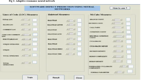
6.1.1 Lines of Code (LOC) measures
The basis of the measure LOC is that program length can be used as a predictor of program characteristics such as effort and ease of maintenance. The LOC measure is used to measure size of the software. LOC is used as DSI (Delivered source Instructions) and KDSI (Thousands of Delivered source Instructions). Only source lines that are delivered as part of the product are included-test drivers and other support software is excluded. The different LOC measure include total LOC, blank LOC, comment LOC, code and comment LOC, executable LOC.
6.1.2 Halstead measures
The Halstead metrics are sensitive to program size and help in calculating the programming effort in months. The different Halstead metrics include length, volume, vocabulary, effort, error, time, level, difficulty, unique operands, unique operators, total operands and total operator. Halstead´s metrics is based on interpreting the source code as a sequence of tokens and classifying each token to be an operator or an operand.
6.1.3 McCabe measures
McCabe metrics measures code (control flow) complexity and help in identifying vulnerable code. The different McCabe metrics include branch count, decision count, call pairs, condition count, multiple condition count, cyclomatic complexity, cyclomatic density, decision density, design complexity, design density, normalized cyclomatic complexity and formal parameters.
6.1.4Preprocessing of dataset:-
The data in the dataset has been normalized in the range [0,1]
using the formula given below:
, ,
,
i j i j
i j
a
a
a
for all 0≤i≤121 ; 0≤j≤297. NEURAL NETWORK
Adaptive resonance theory (ART) models are neural networks that perform clustering, and allow the number of clusters to vary the size of the problem. The major difference between ART and other clustering methods is that ART allows the user to control the degree of similarity between members of same cluster by means of a user-defined constant called the vigilance parameter. ART networks have been used for many pattern recognition tasks, such as automatic target recognition and seismic signal processing.
7.1 Structure of the ARNN
32 ART2 accepts continuous valued vectors. ART2 has highly
complex input processing units. The input processing units if ART2 of normalization and noise suppression, along with the comparison of weights needed for reset mechanism. ART2 has two types of continuous valued inputs. One is called noisy binary posses combination signal and the other truly continuous. The first one can operate with the fast learning type data. The second type of data is more suitable with the slow learning mode. The architecture of ART2 is show in figure 1. Other parameters used are shown in table1.
Fig 1: Adaptive resonance neural network
Table1. Parameters used during training
S.no. Parameter Value
1. Training algorithm ART2
2. Training mode slow learning
3. Input layer units 29
4. Cluster (output) units 02
5. Number of records used in Training 121
8. EVALUATION AND DISCUSSION
This section presents the methodology used in conducting experiments and discusses the results obtained when we applied our proposed neural network to software defect dataset. The analysis undertaken in this study and the dataset used in this work are from PROMISE dataset repository, a publicly available dataset which consists of 93 NASA projects.
The GUI for the software defect predictor is shown in figure 2.
Fig2. GUI of the software defect predictor
Typically the performance of a binary prediction model is summarized by the so called confusion matrix, which consists of the following four counts:-
1. Number of defective modules predicted as defective (true positive i.e. tp)
2. Number of non-defective modules predicted as defective (false positive i.e. fp)
3. Number of defective modules predicted as non-defective (true negative i.e. tn)
4. Number of defective modules predicted as non-defective (false negative i.e. fn)
One may desire tp and tn to have larger values and fp, fn to be smaller but we can measure it using certain parameters defined as follows:-
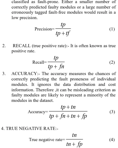
33 classified as fault-prone. Either a smaller number of
correctly predicted faulty modules or a large number of erroneously tagged fault-free modules would result in a low precision.
Precision= (1)
2. RECALL (true positive rate):- It is often known as true positive rate.
Recall= (2)
3. ACCURACY:- The accuracy measures the chances of correctly predicting the fault proneness of individual modules. It ignores the data distribution and cost information. Therefore ,it can be misleading criterion as faulty modules are likely to represent a minority of the modules in the dataset.
Accuracy= (3)
4. TRUE NEGATIVE RATE:-
True negative rate= (4)
We have compared the model with other related purposed
models and the experiments show that the recall of our model
is much better than other models. The comparision results are
shown in Table2.
Table 2: Comparison of Results
Models Precision Recall Accuracy tn rate ARNN 0.54 1 0.1479 0.076
FIS 0.4783 0.9167 0.7292 0.6667
CT 0.4762 0.83333 0.7292 0.6944
LR 0.6154 0.6667 0.8125 0.8611
NN 0.6000 0.5000 0.7917 0.8889
We can see that the Recall of the ARNN model for defect prediction is 100% which is best out of any defect predicting model that has been recently developed. As we can see in table the best recall is of FIS model which is 91.67%. The ARNN model ensures that the defected modules will de detected as defected. When we test software for detecting defected modules we want that all the defected modules should be detected as defective but if recall is low then it may happen that a defective module fall in defect-free module category which will later can produce incorrect results while implementing the software. But in case of ARNN model, this problem will not occur. But due to low accuracy it may happen that some of the defect-free modules fall in defected module cluster but it create no problem when we implement the software as during testing this problem will be solved. This study needs to be extended for the validation using more datasets.
8. CONCLUSION
Software defect prediction continues to attract significant attention as it holds the promise for improving the effectiveness and offering guidance to software verification
and validation activities. Over the past five years, several datasets describing module metrics and their fault content became publicly available. As the result, numerous methodologies for software quality prediction have been proposed in search of “the best” modeling technique. The suggestion to experiment with different modeling techniques followed by the selection of the most appropriate one has become common. Performance comparison between different classification algorithms for detecting fault-prone software modules has been one of the least studied areas in the empirical software engineering literature. We have applied Adaptive Resonance Neural Network for the purpose of defect-prediction in software programs. The network is special case of unsupervised learning so it gets trained as we present new patterns. It recognizes the defect prone modules very effectively. The results produced by this ARNN may vary for different datasets. It helps to reduce the efforts and cost of developing software as it gives prior knowledge of modules containing defects.
9. REFRENCES
[1] M. Bahrololum, E. Salahi, and M. Khaleghi, 2009, Anomaly Intrusion Detection Design using Hybrid of Unsupervised and Supervised Neural Network, International Journal of Computer Networks & Communications pp. 26-33.
[2] Venkata U.B. Challagulla, FarokhB.Bastani,I-Ling Yen2005 ”Empirical Assessment of machine learning based software defect prediction techniques”.Words’05 Proceedings of the 10th IEEE International Workshop on Object-Oriented Real-Time Dependable Systems pp 263-270,.
[3] Mie MieThetThwin,Tong-SengQuah2003 “Application of neural networks for software quality prediction using object-oriented metrics” ICSM '03 Proceedings of the International Conference on Software Maintenancepp116.
[4] NcahiappanNagappan2005”Static Analysis Tools as early Indicators of pre-release defect density” ICSE '05Proceedings of the 27th international conference on Software engineering pp 580-586.
[5] Rudolf Ramer, Klaus Wolfmair,ErwinStauder, Felix Kossak and Thomas Natschlager 2009 “Key Questions in Building defect prediction models in practice”Software Competence Center HagenbergSoftwarepark 21, A-4232 Hagenberg, Austria, pp. 14–27.
[6] Zeeshan Ali Rana,Mian Muhammad Awais and ShafayShamail 2009 ”An FIS for early defect prone modules”Springer-Verlag Berlin Heidelberg ,pp. 144–153.
[7] G. Boetticher, T. Menzies, and T. Ostrand, PROMISE Repository of Software Research Laboratory (Softlab),Bogazici University, Istanbul, Turkey, 2007, http://promisedata.org/ repository.
[8] K. Mehrotra, C. K. Mohan, and S. Ranka, Elements of Artificial Neural Networks (Massachusetts Institute of Technology, MA, 2000).
[9] Martin Neil and Norman Fenton 1996 “ Predicting software quality using Bayesian Belief Networks”. [10] Todd L. Graves, Alan F. Karr, J.S. Marron and Harvey
Siy 2000 “Predicting Fault Incidence Using software change history”. IEEE transactions of software engineering.