Hardy-Weinberg Testing for Continuous Data

(1)

Copyright D 1997 by the Genetics Society of America

Hardy-Weinberg

Testing for Continuous Data

Lauren

M.

McIntyre’

and

B. S.

Weir

Program in Statistical Genetics, Department of Statistics, North Carolina State University, Raleigh, North Carolina 27695-8203 Manuscript received June 29, 1996

Accepted for publication August 27, 1997

ABSTRACT

Estimation of allelic and genotypic distributions for continuous data using kernel density estimation is discussed and illustrated for some variable number of tandem repeat data. These kernel density estimates provide a useful representation of data when only some of the many variants at a locus are present in a sample. Two Hardy-Weinberg test procedures are introduced for continuous data: a continu-

ous chi-square test with test statistic TCa and a test based on Hellinger’s distance with test statistic Tm. Simulations are used to compare the powers of these tests to each other and to the powers of a test of intraclass correlation TIC, as well as to the power of Fisher’s exact test T ~ T applied to discretized data. Results indicate that the power of TCcs is better than that of THDt but neither is as powerful as TET. The intraclass correlation test does not perform as well as the other tests examined in this article.

F

ROM MENDEL’S work onward, the language of population genetics has usually been phrased in terms

of loci with discrete alleles, and a rich body of theory has been developed to analyze discrete genetic data (reviewed in WEIR 1996). With molecular technology now making available DNA sequences for population studies, the dominance of discrete data might be thought to be complete. Paradoxically, however, molecular techniques have often introduced uncertainty into allelic designations. Whenever alleles are detected elec- trophoretically, there is uncertainty in the relationship between measured migration distances and inferred fragment lengths. Although this was recognized when protein variants were the primary type of population genetic data, there were usually so few alleles at a locus that there was little trouble in distinguishing between them. Measurement error was not an important consideration. The more recent introduction of minisatellite markers, especially the variable number of tandem repeat (VNTR) loci employed for individual identifica- tion, has revealed such a high degree of variation, with hundreds of alleles, that allelic differences cannot be determined with certainty from fragment length differences. At locus DlS7, for example, the repeat length is 9 bp and estimated fragment lengths between 600 and 22,000 bp are found in samples from human populations. It is not possible to distinguish all 2300 alleles

by electrophoresis and the estimated fragment lengths should be considered as continuous data, notwithstand- ing the fact that they represent integral numbers of

Corresponding author: Lauren McIntyre, Division of Biometry, Duke

Univelsity Medical Center, Box 3827, Durham, NC 27710. E-mail: [email protected]

h s m t address: Veterans’ Administration Medical Center, 508 Fulton St., HSR&D (152), Durham NC 27705 and Duke University Medical Center, Division of Biometry, Department of Community and Family Medicine, Durham, NC 27710.

Genetics 147: 1965-1975 (December, 1997)

repeat units and are usually reported as integers. The estimate of the fragment length is a function of the true size and measurement error.

The effect of the measurement error on estimated fragment lengths has been addressed by DEVLIN et al. (1991) and EVETT et al. (1993). Not only does measurement error obscure allele definition, but also if a hetero- zygous individual has two fragments of similar length, the fragments may coalesce and appear on the gel as a single fragment rather than two distinct fragments (DEVLIN et al. 1991). Sometimes coalescence can be resolved by modifying electrophoretic conditions, but in this paper we ignore the coalescence problem and concentrate on allele definition.

Even with measurement error obscuring some allele definition, VNTR markers have an incredible amount of variation and this makes them of great use for identi- fication. It also makes analysis of population data difficult. One approach to analyzing continuous population genetic data is to apply a discretization process. In essence, this is what was done with protein variants. The additional variation sometimes revealed by changing electrophoretic conditions (JOHNSON 1976) was hidden by the few alleles seen under standard conditions. Dis- cretization is made explicit by the “binning” techniques used by forensic scientists (e.g., BUDOWLE et al. 1991). Fragment lengths at DlS7, for example, are as- signed to the 31 intervals, or bins, between successive bands on a sizing ladder. Such strategies have the advan- tage of simplicity, although there can still be ambiguity over which discrete allele is appropriate for a particular fragment length. More importantly, the resulting discrete data can be analyzed with traditional methods.

(2)

1966 L. M. McIntyre and B. S. Weir

nize the nature of the data. Several such analyses have appeared in the forensic literature (BERRY 1991; BUCK- LETON et al. 1991; EVETT et al. 1993; HARTMANN et al.

1994; AITKEN 1995). These analyses use kernel density estimation as a way of estimating allelic distributions for use in the calculation of profile frequencies. However, these papers generally assume Hardy-Weinberg equilib rium and do not address testing for Hardy-Weinberg equilibrium in a continuous framework. Inference about independence of allelic frequencies at single loci from a continuous viewpoint has previously been in terms of correlation coefficients (WEIR 1992a,b; CHA-

KRABORTY et al. 1993; HAMILTON et al. 1996).

Because of the potential use of continuous data in population genetic studies (PROUT and BARKER 1994), we explore some continuous analyses here. This work also responds to the call by the NATIONAL RESEARCH COUNCIL (1996) for research into methods for analyzing continuous genetic data. In particular, we show how both allelic and genotypic data may be represented by “smoothed” distributions, and then we compare genotypic distributions with products of allelic distributions to provide a continuous analogue of the traditional tests for Hardy-Weinberg equilibrium. We focus on kernel density smoothing and find that test statistics of the Rosenblatt-Bickel type (BICKEL and ROSENBLATT 1973) perform well, although not as well as tests on discretized data. We illustrate the procedures by applying them to some simulated databases.

THE DATA

Although this work was motivated by the need to accommodate VNTR data, the general approach ap- plies to any locus where the variants are described by continuous measurements. For a VNTR locus, a sampled individual has a pair of estimated lengths X, Y. Although there is generally no way to determine parental origin of these two lengths, it is convenient to use the different symbols and denote heterozygotes by both X, Y and Y , Xwhen X # Y. We will use Xwhen referring to just one of the lengths. The lengths are considered to be related to the number a of repeat units, in the simplest model that ignores flanking regions, by

x =

TU

+

E , ( 1 )

where ris the length of the repeat unit and E is an error term. We assume that r is constant within and between individuals. Several authors have discussed the distribution of errors E (BUCKLETON et al. 1991 ; DEVLIN et al. 1991; EVETT et al. 1993). Measurement errors have been found to be skewed and also to depend on the lengths of the fragments. However, measurement errors are a small fraction of the total fragment lengths (-2% according to EVETT et al. 1993) and a strong dependence among measurement errors need not cause a strong dependence among fragment lengths within or be-

tween individuals. We will concentrate on tests for dependence between the two fragment lengths per locus within individuals without seeking to deconvolve or sep- arate the error term from the true length of the repeat unit.

ALLELIC AND GENOTYPIC DENSITY ESTIMATION

For discrete data, tests of the Hardy-Weinberg law depend on comparisons of genotypic frequencies (strictly, sample proportions serving as estimates for population probabilities) with appropriate products of allelic frequencies (MAISTE and WEIR 1995). We wish to adopt the same general strategy for continuous data, but need to work with probability density functions rather than discrete probabilities. For highly variable loci, unless samples are much larger than is usually the case, empirical density functions are very “spiky” for both genotypes and alleles. For this reason we have chosen to smooth these empirical functions before conducting Hardy-Weinberg tests.

Empirical density functions, whether or not they are smoothed, are analogous to histograms for discrete data. For a discrete locus with m alleles, the m allelic counts can serve as the heights of bars in a histogram and the histogram itself provides a nonparametric estimate of the probability distribution. It is also possible to construct a histogram, with m(m

+

1)/2 bars, for the set of genotype counts and of course it is the genotype counts that are summed to provide allele counts. An-

other histogram of expected counts could be constructed, from the Hardy-Weinberg relation, to provide a graphical indication of whether the sample supports Hardy-Weinberg. The observed and expected genotypic histograms could be constructed in three dimensions, as shown in Figure 1. Unless maternal and paternal alleles can be distinguished, these bivariate histograms must be symmetric about the diagonal whose elements represent homozygote counts.

If continuous data are discretized by binning, con- struction of histograms needs to consider the issue of the number and the width of the bins (histogram bars). The bins are not specified as they are in the discrete case and could be chosen to be of equal width (B-S et al. 1989), equal frequency (GEISSER and JOHNSON 1992, 1995; WEIR 1993), or by some external means (BUDOWLE et al. 1991). Once bin widths and boundaries have been determined, the data can be sorted into the bins. The number of occurrences for each bin serves as the height of the histogram bar for that bin.

(3)

Continuous Hardy-Weinberg Testing 1967

AA AB AC BB BC cc

C

A c '

FIGURE 1.-An example of histogram estimates for blood group data. (A) An histogram for allelic blood group data. (B) An histogram for genotypic blood group data. (C) A

bivariate histogram for genotypic blood group data

et al. 1993; HARTMANN et al. 1994; AITKEN 1995). Addi- tionally, it is easy to ensure positive density estimates with the kernel approach. Kernel density estimation has been reviewed in general by SILVERMAN (1993) and for VNTR loci by AITKEN (1995). We now consider univariate density estimation for allele frequencies and bivariate estimation for genotype frequencies.

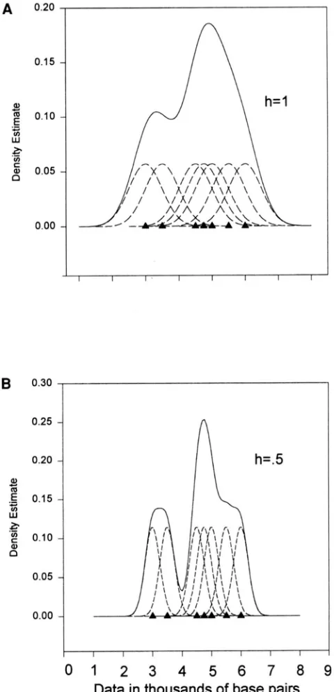
Univariate kernel density estimation: The essence of kernel density estimation is to impose upon each data point a distribution or kernel density. The estimated density at any point along the range of the data is the sum of all the overlapping kernel densities at that point. The procedure is shown graphically in Figure 2 for a trivial case of a sample of size seven. The seven data points are filled triangles, the kernels are shown as dot- ted curves, and their sum forms the kernel density shown as a solid line. In this example a normal kernel with the mean equal to the observed data point and a common standard deviation was used.

For a fragment length of x, the general form of a univariate kernel density estimate f n ( x ) of the continuous probability density functionJx), based on a sample of n values

Xi,

i = 1, 2,

.

. .

, n, is

B

0.30

0.25

0.20

9

.E 0.15

.-

0

E

0.10 n

m

W

-

u)

a,

0.05

0.00

1 I I I I I I I

0 1 2 3 4 5 6 7 8 9

Data in thousands

of

base pairs

FIGURE 2.-How to use kernel density estimation to make a nonparametric density estimate. (A) Kernel estimator with smoothing parameter h = 1. (b) Kernel estimator with smoothing parameter h = 0.5.

where K is the kernel function, and h is known as the bandwidth or smoothing parameter. Under the conditions h + 0, and nh + UJ as n + 03, the kernel density

estimate will converge in probability to the true density (SILVERMAN 1993).

(4)

1968 L. M. McIntyre and B. S. Weir

elected to use a normal kernel that is not changed over the range of the data (Figure

2).

The normal kernel is

+)

x - x

-

e - ( * X i ) w . (3)

Equations 2 and 3 provide the kernel density estimate at a single point x. If many points along the range of interest are examined, a very clear representation of the density function can be achieved. Making the grid finer, or increasing the number of points at which the density is evaluated, will increase the resolution. All density estimation in this paper used grids of equally spaced points over the range of the data. Generally, we used a grid of 50 intervals for allelic density estimates, and a two-dimensional grid of 50 X 50, or 2500 intervals, for genotypic density estimates.

The choice of kernels has been discussed and reviewed by GHOSH and HUANC (1991) and SILVERMAN

(1993). These authors have found the normal kernel to be efficient, and they found that choosing a different symmetric kernel does not appear to have much impact on the efficiency of the estimated density. The width of the kernel is affected by h, which is the standard deviation of the normal kernel in Equation 3. This parameter has a major effect on the analysis and is analogous to the width of the bars in a histogram. In Figure

2B the same data were used as in Figure 2 A , but a bandwidth of h = 0.5 was used instead of h = 1. A larger bandwidth will produce a smoother density estimate, which explains the term “smoothing parameter.”

For the VNTR data in this study h was kept the same over the entire range of the data. In cases where the tails of the distribution are long, a small h for the entire density estimate can result in noise in the tails of the estimated density. However, if one tries to smooth the tails by increasing h, the central part of the density may be overly smoothed. One solution is to vary h along the range of the data. Another solution is to transform the data: a logarithmic transformation has the same effect as increasing h along the range of the data. We have not varied h or transformed the data in this study as there were no long tails in these simulated distributions. However, the methods described in this paper can be applied to transformed data. HARTMANN et al. (1994) did allow h to vary along the range of the data.

Note that our choice of a kernel is not related to the measurement errors associated with fragment lengths, even though these errors may coincidentally have a normal distribution. The lengths

X

already include the measurement error (Equation 2), and it is the density for the overall length (the sum of the true length plus the error) that is to be estimated. If it was desired to formulate a density estimate of the number of repeats

r, then some deconvolution process would have to be implemented (LIU and TAYLOR 1989), based on a model for the errors E . Therefore, the choice of a kernel

depends on concerns such as efficiency of calculation and existence of derivatives of all orders rather than the structure of the measurement error E . Although

there are many automatic methods for choosing h, since the effect of h on Hardy-Weinberg testing procedures was not known at the outset, several “reasonable” values were used.

As

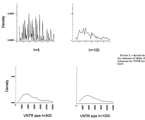
an example, we show in Figure 3 the kernel density estimates from a sample of 610 fragment lengths from 305 African-American individuals for locus D1S7 col- lected by the Broward County Crime Laboratory, Flor- ida (individuals with only one length were omitted from the analysis). It can be seen that the estimate for h = 5 was still very spiky, and the estimate for h = 1000 was

so smooth as to have lost much information. Reason- able choices appear to be in the range h = 100

-

500

for this locus. SILVERMAN (1993) has a standardization of h / s allowing a comparison of h values for different data sets. For this example h / s gives values of 0.034

-

0.17.

Bivariate kernel density estimation: Each individual has two fragment lengths so a bivariate distribution

f i x , y) is needed for genotypic distributions. Univariate methods are easily extended to provide a bivariate density estimate at gridpoint x, y:

where X;, are the fragment lengths for the

ith

individual, i = 1, 2,

.

. . ,

n. For the bivariate kernel estimate to converge in probability to the true density it is necessary that h + 0, and nh2 + co as n -+ m. We use a bivariate

normal kernel with zero correlation between the two variables:

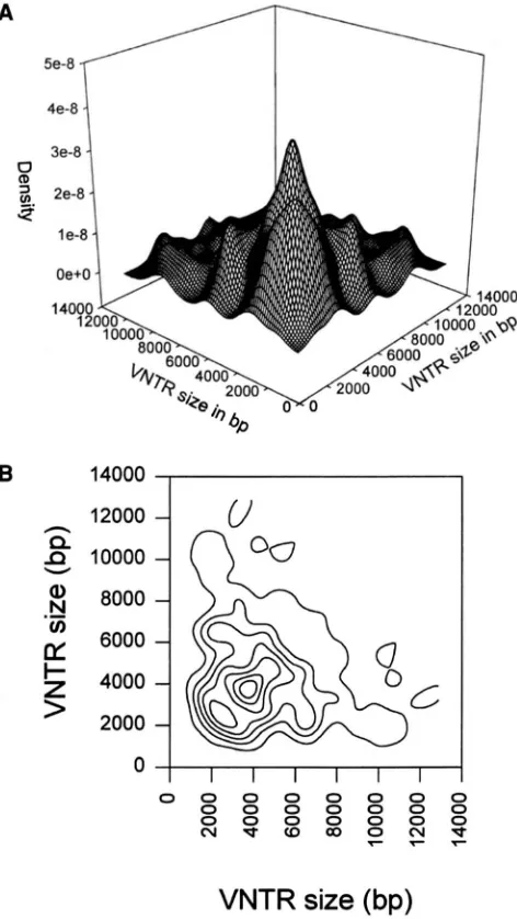
An example of the genotypic density estimate for the Broward County D1S7 data is shown in Figure 4, both

as a surface and as a contour plot. These figures may be easier to interpret than the corresponding bivariate histogram.

HARDY-WINBERG HYPOTHESIS

Consider a locus with discrete alleles Ai having fie- quencies

pi,

and genotypes A d j having frequencies Pij. The Hardy-Weinberg relation, if heterozygote frequencies are written as Pv

+

q , is as follows:

(5)

Continuous Hardy-Weinberg Testing 1969

0.0005

i

_I

I

0.0000

h=5

VNTR

size

h=500

where Ax, y) is the bivariate density for genotypes with fragment lengths x, y, and A x ) is the univariate density for length x. Equation 7 is the usual definition of independence for variables X, Y , and it suggests a test procedure. Using data on 1~ individuals, the genotypic kernel density estimatef,(x, y) expected under the null hypothesis of Hardy-Weinberg equilibrium is calculated as the product of the allelic kernel density estimates f n ( x) and

fn(y). Note that the functional forms of f n ( x ) and f n ( y )

are the same since the parental origin of the alleles is considered not to affect frequency distributions.

Alternative hypothesis: The evaluation of different testing strategies will be based on power considerations, and this requires the specification of an alternative hypothesis. A convenient alternative in the discrete case is phrased in terms of the within-population inbreeding coefficient f =

F&

All alleles are treated alike, so that there is only one

h=lOO

FIGURE 3.-Kernel den- sity estimates of allelic distributions for VNTR locus

DlS7.

VNTR

size

h=lOOO

value off Testing against this alternative refers just to the population sampled, and no evolutionary implica- tions can be drawn. In the language of WEIR (1996), the analysis is for a “fixed” population. To address the issue of dependence imposed by population structure, when allele and genotype frequencies both refer to a total population consisting of a series of subpopulations, it is necessary to replace f by F =

Fni

the total inbreeding coefficient, and the analysis is now for “random” populations. For random-mating populations, the total inbreeding coefficient is the same as the coancestry coefficient,

F

=

8(Fn

=

FsT). The inbreeding coefficient

Fm

is the probability that two alleles within one individual are identical by descent (ibd), whereas the coancestry 8 is the probability that two alleles in two different individuals are ibd. Both measures are aver- aged over subpopulations. Although the analysis we present is meant to be within populations, we use 8 in place off in Equation 8 to avoid confusion with density function notation.

(6)

1970

A

L. M. McIntyre and B. S. Weir

TESTING PROCEDURES

We have examined two tests for independence of continuous distributions: a specific form of the Rosen- blatt-Bickel test (ROSENBLATT 1975) and a test based on Hellinger's distance (KOTZ andJoHNsoN 1981). We have examined the effects of h and of 0, as well as of the range of the data and the underlying marginal allelic distribution on the power of each of these two tests. We have also tested for the presence of intraclass correlation and we have applied Fisher's exact test. In tests for Hardy-Weinberg we expect the test statistic to be affected by the value of 0 and we point out this effect in the discussion of the test statistics.

Continuous chi-square test: BICKEL and ROSENBLATT (1973) presented a univariate test statistic that was the continuous analog of the chi-square goodness-of-fit test.

ROSENBLATT (1975) gave the two-dimensional exten- sion and showed the distribution of the test statistic under the null was normal, with mean and variance depending on h and the range of the data in the case of a uniform [0, 11 marginal distribution. We do not invoke this asymptotic distribution of the test statistic, but rely instead on the permutation procedure, described in the numerical procedures section, to determine power and significance levels.

We refer to the test as the continuous chi-square test, CCS, and note that it is based on the quantity

B 14000

1

12000

A

In"

10000 v

8

8000

K

6000

4000

.-

0

'

2000

0 0 0 0 0 0 0 0

0 0 0 0 0 0 0

N

-

r

u

3 a

~

g

~

VNTR size (bp)

FIGURE 4.-Kernel density estimates of genotypic distribu- tions for VNTR locus DlS7. (A) Surface plot. (B) Contour plot.

In other words, the joint density is (1

-

6 ) times the product of the two marginal densities everywhere on the x, y plane, plus an additional term of 0 times the common marginal density on the line x = y. Evidently, 0 is the intraclass correlation for fragment lengths within individuals, and under the alternative in Equa- tion 9 a test for an intraclass correlation coefficient larger than zero is a test for Hardy-Weinberg equilibrium. However, there are cases where the data may be uncorrelated but not in Hardy-Weinberg equilibrium. The intraclass correlation is zero in this scenario, although clearly the two fragment lengths are not inde- pendent.

The unknown density functions are replaced by kernel density estimates, and the numerator is expanded to

provide

We evaluated this integral numerically by evaluating the function at each point of the twodimensional grid used for the kernel density estimate, multiplying by the (equal) grid widths dx and dy and adding all these terms together. For computational purposes it is possible to drop the constants nh2, -1, and dx, dy and write the test statistic as

Tea:

This test statistic increases as 0 increases.

(7)

Continuous Hardy-Weinberg Testing 1971

bandwidths can similarly be increased. In that case, a shrinkage in the test statistic is observed.

Hellinger’s distance test: Hellinger’s distance ( KOTZ and JOHNSON 1981) provides a means of comparing two density functions by means of a quantity bounded between zero and one. To compare bivariate functions

fI

x, y) and

g(

x, y) , the distance

HD

is calculated as

H.D =

[

s,

( G - 3 - h r ) Z d x d y ]

1/2

=

[

2

-

2

s,

m d x d Y ] l ’ z . (11)

If &(x, y) is a bivariate kernel density estimate and

fn(x)fn(y) is the product of the kernel density estimates of the two marginal distributions, a Hellinger distance can be calculated between them. From the form of Equation 11, we define a test statistic THD as

X Y

This decreases as 8 increases. Significance levels and power are determined using the permutation procedure described below.

Intraclass correlation coefficient test: An estimator

T I C for the intraclass correlation coefficient was given

by WEIR (1992a). If the fragment lengths in the ith of n individuals are

(X,

x),

this statistic is

where the between-individual and within-individual mean squares are

B =

2(n - 1) n

For the alternative hypothesis in Equation 9, this statistic gives an estimate of 0, so increases with 8. Signifi- cance levels and power are determined using the permutation procedure described below.

Fisher’s exact test: For discrete data, MAISTE and

WEIR (1995) found that Fisher’s exact test FET is the most powerful Hardy-Weinberg test. The exact test uses the conditional probability of genotype counts nq given allelic counts nj. Under the Hardy-Weinberg hypothesis this conditional probability is

where n is the sample size, His the number of heterozygotes in the sample, and the product in the denomina- tor is over all genotypes. Because the statistic is evaluated over datasets obtained by permuting alleles (see

below), it is necessary to keep track only of genotype counts and the test statistic is written as TmT:

2H (2n)!II,(nq!) ‘

This statistic decreases as 8 increases.

In the present study, fragments were placed into discrete bins that were defined arbitrarily to be of equal width b to provide a comparison with the constant h used in tests based on the kernel approach. Significance levels and power are determined using the permutation procedure described below.

Numerical procedure: We have employed simulation to evaluate our procedures, and we used four different fragment length distributions. These four distributions were as follows: (1) uniform over the range 500-8000 bp, (2) normal with a mean of 4250 bp and a standard deviation of 1875 bp, 95% of which lies in the range 500-8000 bp, (3) normal with mean of 6450 bp and a standard deviation of 2775 bp, 95% of which lies in the range 900-12,000 bp and (4) an equal mixture of two normals (one with mean 1000 bp and standard deviation 500 bp and the other with mean 4700 bp and standard deviation 1875 bp), -90% of which lies on the range 500-8000 bp. The range 500

-

8000 bp was chosen because it is close to the range commonly observed for loci D2S44, D10S28 and D5S110. Data simulated from the normal distributions were discarded if they lay outside specified ranges: 500-8000 for (2) and (4), and 900-12,000 for (3). This was done to keep the observations within a predefined grid.

To simulate genotypes, we chose the first fragment length from one of the four distributions, and then with probability 8 made the second fragment identical to the first. With probability 1 - 8, the second fragment length was chosen independently from the same distribution as the first. When 8 = 0 there is independence between fragment length pairs within individuals in the simulated data. In all cases, we used a sample size of n

= 100 individuals.

For each allelic distribution, data were simulated with four different 8 values: 8 = 0, 0.01, 0.05, 0.1. The 8 = 0 cases correspond to the null hypothesis, while the 8

>

0 cases depart from Hardy-Weinberg equilibrium. For each of these simulations the test statistics TCa and

THD were evaluated at three different bandwidths h =

100,250,500. Since the kernel density function fn( x, y)

and the expected genotypic density f , ( x ) f , ( y ) are symmetric, we performed the numerical integrations for the test statistics Tca and THD on half of the grid off the diagonal, as well as at grid points on the diagonal x = y. For Fisher’s exact test, binwidths were assigned three different possible values: b = 100, 250, 500. Note that b is also a smoothing parameter and is the discrete analogue to the smoothing parameter h used in the kernel density estimation. We evaluated the intraclass correlation T I C at each bandwidth as a check on the

(8)

1972 L. M. Mclntyre and B. S. Weir

stability of the simulations; this statistic is not affected

For each test, the significance level was calculated as the proportion of times a new set of n genotype counts, formed by permuting all 2n alleles, gives a more extreme test statistic (GUO and THOMPSON 1992; WEIR 1996). For any set of parameter values, power was determined as the proportion of simulated data sets that had significance levels less than CY = 0.05. In the cases of 8 = 0 (the null hypothesis) we expect the power of all tests to be -5%.

As

8 increases, the power of the test should increase. It is less clear how the different bandwidths/binwidths and the different marginal distributions should affect the power of the tests.

The detailed steps in power calculations were as follows:

1. A data set of 2% = 200 fragment lengths ( n = 100 genotypes) was simulated according to one of the combinations of parameter values.

2. All four test statistics TCcs, Tm, TIC, TmT were calculated (for each value of h for the first three, or each value of b for the fourth).

3. All 2n fragment lengths were then permuted to form a new set of n genotypes.

4. The test statistics Tees, Tm, Tfc, TmTwere then evaluated on the permuted genotypes.

5. Steps three and four are repeated I times to give an empirical distribution under the null hypothesis for each test statistic.

6. The proportion of the Ipermuted values that are as extreme or more extreme than the value from the original data is computed. If this proportion

( p

value) is less than or equal to 0.05, the null hypothesis is rejected.

7.

Steps one through six are replicated 0 times. The proportion of the 0 times that the hypothesis is rejected provides an estimate of power.

A discussion of the values for inner and outer loop numbers I a n d 0 was given by ODEN (1991). If the test is to be applied to one set of real data, then sufficient permutations are needed to provide a good estimate of the significance level and the power. From binomial a 95% confidence interval for

p

is

fi

5 0.96 f i ( 1

-

! ) / I , where

fi

is the observed proportion of permutations giving a test statistic as extreme or more extreme than that for the data. The interval is widest when

p

= 0.5, and then has width of 0.01 each side of

fi

when I = 10,000. ODEN pointed out that I need not be so large in power studies because of all the additional information provided by the 0 outer loops. Provided there is low bias in estimating

p,

the variance of

p

is determined primarily by 0. We set I = 159, so that the hypothesis would be rejected when the test statistic from the data was among the most extreme eight of the 159

+

1 = 160 values. The power of a test is estimated as the proportion of the 0 outer loops in which rejection bY Jl'.

t h e o F " -

occurred. We set 0 = 1350. We took

dB(

1

-

B ) / O as an estimate of the standard deviation of the estimated power

8.

This estimate will provide accurate estimates of power to the first decimal place. As power differences were large, this was determined to be adequate.

We compared tests with McNemar tests: the four out- comes of reject or not-reject for two tests can be re- garded as the cells of a 2

x

2 contingency table and a chi-square test performed. If a, b are the numbers of times the two tests disagree (the first test rejects and the second does not reject in a replicates, and the reverse happens in b cases), the test statistic is M = ( a - b)'/

( a

+

6) and is distributed chi-square with one degree offreedom when the tests have equal performance.

RESULTS

We show power values in Tables 1 and 2. Power is highly dependent on the bandwidth for all methods. This result is consistent with the theory of BLETH

(1993). Similarly, binwidth has a substantial effect on the power of Fisher's exact test. Interestingly, choosing the bandwidth based on automatic procedures will not always lead to the most powerful test. When conducting tests for Hardy-Weinberg equilibrium, therefore, we should not only be aware of the effect of binwidth/ bandwidth on the power of the tests but also realize that we can choose a binning strategy to maximize the power of detecting departures from Hardy-Weinberg. Adding a consideration of power to the choice of bandwidths has also been suggested by BLYTH (1993).

The effect of the 8 parameter on the power is also substantial, and there is low power for detecting 6

<

0.05. This is consistent with the findings of MAISTE and WEIR (1995). Increasing the range of the data seems to increase the power for certain bandwidths, as was found by MCINTYRE (1996) (this thesis contains results for the parameter sets not shown in Tables 1 and 2, and a copy may be obtained from the author). This is expected from work of BICKEL and ROSENBLATT (1973) showing that the mean and variance of the test statistic depends on both the range of the data and the bandwidth.

We used analyses of variance to test for effects of the factors h, 8, marginal distribution and range on the power of the tests. Although the empirical powers are not normally distributed, we consider that analysis of variance will provide an indication of the impact of the four factors. For all tests, the parameters h and 8 had a highly significant effect on the power and so did the interaction between h and 8. However, the allelic distribution and range of data seemed to have no significant impact on power.

The McNemar tests indicated that tests based on TK.E and THD are significantly different and Tccq was also more powerful than T I C .

(9)

Continuous' Hardy-Weinberg Testing

TABLE 1

Power of tests for fragment lengtbs distributed udifarmly OVCT the range 500-8000 bp

e

h , b

ccs

HD IC

FET

0.00 100 0.050 (0.006) 0.044 (0.006) 0.055 (0.006) 0.063 (0.007)

250 0.062 (0.007) 0.044 (0.006) 0.067 (0.007) 0.051 (0.006) 500 0.047 (0.006) 0.041 (0.005) 0.039 (0.005) 0.040 (0.005)

250 0.070 (0.007) 0.047 (0.006) 0.066 (0.007) 0.068 (0.007) 500 0.059 (0.006) 0.035 (0.005) 0.040 (0.005) 0.061 (0.007) 0.05 100 0.217 (0.011) 0.097 (0.008) 0.086 (0.008) 0.748 (0.012) 250 0.141 (0.010) 0.069 (0.007) 0.109 (0.009) 0.330 (0.013) 500 0.109 (0.009) 0.059 (0.006) 0.106 (0.008) 0.182 (0.011)

0.10 100 0.564 (0.014) 0.287 (0.012) 0.192 (0.011) 0.991 (0.003) 250 0.328 (0.013) 0.154 (0.010) 0.199 (0.011) 0.765 (0.012) 500 0.239 (0.012) 0.119 (0.009) 0.190 (0.011) 0.492 (0.014) 0.01 100 0.071 (0.007) 0.042 (0.006) 0.057 (0.006) 0.191 (0.011)

SD is indicated in parentheses.

1973

the bandwidth for the kernel estimate are parameters that have the same effect, the kernel is based directly on the data points, while the histogram is based on the bins. It has been suggested that h is equivalent to the binwidth (SCOTT 1979). If the h parameter for the kernel estimate is taken to be exactly equal to the binwidth b and the simulation results are compared for this scenario, Tm is almost twice as powerful as Tca in all cases. It has also been suggested that h for the kernel estimator is equivalent to half the binwidth h = b / 2 for the histogram ( SILVERMAN 1993), If this were the case, a comparison of the simulation results shows that TmT still seems to be more powerful in most cases, although the difference in powers between Tm and Tca is much less extreme when this comparison is made. Therefore, it is perhaps more correct to say that the power for Tm and the power for Tca are affected by the smoothing parameter and the smaller the value of the parameter, the higher the power.

For the alternative hypothesis in Equation 9, TIC in-

creases with 8, whereas

Tees

increases with

@.

For the alternatives with disequilibrium but uncorrelated fi-ag- ment lengths, however, the IC test is not appropriate.

CONCLUSION

VNTR data are highly polymorphic, and this large amount of variation makes analyses of data from these loci both difficult and complex. The usually simple task of defining alleles is no longer straightforward.

While discretizing the data certainly gives allelic and genotypic frequency estimations, the method of discretization can profoundly impact the actual frequency estimates (WEIR 1993). Continuous approaches to frequency estimation for

VNTR

data have been proposed by AITKEN (1995), BERRY (1991), BUCKLETON et al.

(1991),EvEmelal. ( 1 9 9 3 ) , H A R ~ ~ ~ ~ ~ e t a l . (1994)and MORRIS et al. (1989). A good discussion of using a kernel approach to estimate frequencies of genotypes was given by EVETT et al. (1993), under the assumption of

TABLE 2

Power of tests for fragment lengths distributed normally over the range 500-8000 bp

e

h, b

ccs

HD IC E T

0.00 100 _{0.061 (0.007)} _{0.046 (0.006)} _{0.046 (0.006)} _{0.064 (0.007)}

0.01 100 0.082 (0.008) 0.048 (0.006) 0.066 (0.007) 0.164 (0.010) 250 0.059 (0.006) 0.041 (0.005) 0.048 (0.006)

500 0.036

(0.005) 0.049 (0.006) 0.043 (0.006) 0.057 (0.006) 0.043 (0.006)

250 0.070 (0.007) 0.051 (0.006) 0.055 (0.006) 0.064 (0.007)

500 0.049 (0.006) 0.043 (0.006) 0.058 (0.006) 0.043 (0.006)

0.05 100 0.216 (0.011) 0.113 (0.009) 0.106 (0.008) 0.710 (0.012) 250 0.181 (0.011) 0.076 (0.007) 0.109 (0.008) 0.298 (0.012) 500 0.110 (0.009) 0.061 (0.007) 0.101 (0.008) 0.187 (0.011)

0.10 100 0.492 (0.014) 0.284 (0.012) 0.211 (0.011) 0.970 (0.005)

250 0.374 (0.013) 0.179 (0.010)

500

0.195 (0.011) 0.288 (0.012)

0.696 (0.013) 0.156 (0.010) 0.200 (0.011) 0.445 (0.014)

(10)

1974 L. M. McIntyre and B. S. Weir

independence of alleles within a locus. Likewise, HART- MANN et al. (1994) developed a kernel approach to the estimation of allele frequencies.

Allele and genotypic frequency estimates are crucial for attaching weight to evidence of matching DNA pro- files

EVE^

et al. 1993; AITKEN 1995). Almost all methods for assessing weight have assumed Hardy-Weinberg equilibrium. TO date the discussion of Hardy-Weinberg independence has been limited to the case where VNTR data are discretized and then tested, or where independence

has

been addressed via intraclw correlations. This article describes one way of estimating allelic and genotypic densities and performing tests for Hardy- Weinberg equilibrium based on a continuous approach.

We used kernel density estimation to estimate allelic and genotypic frequencies. This has many advantages, including being easily understood and implemented. More importantly, the mean integrated squared error, MISE, of the univariate kernel estimator approaches zero faster than the MISE for the histogram estimator. The asymptotic properties of the kernel are thus better than those for the histogram. We also believe the kernel estimator to be visually more pleasing, and in the bivariate case to be easier to interpret than the bivariate histogram. The real utility for the kernel estimator, in this context, seems to be in facilitating the estimation of genotypic and allelic densities. Since binning strategies are avoided, the kernel estimator alleviates concerns about the placement of an individual into an incorrect bin. The choice of an appropriate binwidth or bandwidth can be explored as an optimization problem

where the MISE is minimized and the power of the test maximized.

The performance of Hardy-Weinberg tests based on the continuous kernel estimator

Tees

and THD are af-

fected by the choice of the smoothing parameter and the coefficient 8, as is Fisher’s exact test. TCa is more powerful than THD. While exact correspondence between binwidth and bandwidth is not clear, the results show that, at best, Tcm has equal power to T m , and Tm is not as powerful as TCm. With the fast computation methods of GUO and THOMPSON (1992) and Z A m N et

al. (1995), TmT is much less computer intensive than either Tccs or T,. This seems to indicate that there is no compelling reason to use T c ~ over TmT in terms of power of the test against the alternatives considered here. For alternatives where there is dependence but no correlation, TIC should not be used and in fact is not as powerful as either Tcm or TET. In practice, of course, the nature of any actual departure from Hardy- Weinberg is not known.

We have clearly demonstrated the impact of the parameter h on testing for Hardy-Weinberg equilibrium. The smaller values of h lead to higher power for all tests, but do not change the bias/variance relationship between the estimates and h. Additionally, there are

limits on the size of the bandwidth that is appropriate for the data at hand to avoid under- or oversmoothing. Traditional “plug in” estimators can be used as a start- ing point for determining the reasonable range of h. Then if testing for independence of fragment lengths is the objective, a smaller bandwidth should be used keeping in mind the bias and variance of the estimates. If the main goal is to provide an accurate estimate of continuous genotypic and allelic densities, then h should be varied over the informative range to gain as much insight into the behavior of the variables as possible.

Broward County Crime Laboratory data were made available by Dr. GEORGE DUNCAN. Dr. DOUGLAS NYCHKA offered substantial help. This work was supported in part by National Institutes of Health grant GM45344, by U.S. Department of Education Patricia Roberts Harris fellowship program, and by U.S. Department of Education Graduate Assistance in Areas of National Need Interdisciplinary fellowship program in biotechnology.

LITERATURE CITED

AITKEN, C. G. G., 1995 Statistics and theEvahatdon o f E u i h c e fwFwen-

sic Scientists. Wiley, New York.

BAIAZS, I., M. BAIRD, M. CLYNE and E. MFADE, 1989 Human population genetic studies of five hypervariable DNA loci. Am. J. Hum. Genet. 44: 182-190.

BERAN, R, 1977 Minimum Hellinger distance estimates for pamnet- ric models. Ann. Stat. 5: 445-463.

BERRY, D. A,, 1991 Inferences using DNA profiling in forensic iden- tification and paternity cases. Stat. Sci. 6: 175-205.

BERRY, D. A., I. W. EVEIT and R. PINCHIN, 1992 Statistical inference in crime investigations using deoxyribonucleic acid profiling.

BICKEL, P. J., and M. ROSENBLATT, 1973 On some global measures of the deviations of density function estimates. Ann. Stat. 1:

1071-1095.

BLVH, S., 1993 Optimal kernel weights under a power criterion. J.

BUCKLETON, J., IC A. J. WALSH and C. M. TRIGGS, 1991 A continuous model for interpreting the positions of bands in DNA locus- specific work. J. Forensic Sci. Soc. 31: 353-363.

BUDOWLE, B., A. M. GIUSTI, J. S. WAYE, F. S. BAECHTEL, R M. FOURNEY

et aL, 1991 Fixed-bin analysis for statistical evaluation of continuous distributions of allelic data from VNTR loci, for use in forensic comparisons. Am. J. Hum. Genet. 48: 841-855. CHAKRABORTY, R., M. R. SRINNASAN and M. DE ANDRADE, 1993 In-

traclass and interclass correlations of allelic sizes within and between loci in DNA typing data. Genetics 133: 411-419. DEVLIN, B., N. RISCH and K ROEDER, 1991 Estimation of allele fre-

quencies for VNTR loci.

Am.

J. Hum. Genet. 4 8 662-676. EVEIT, I. W., J. SCRANAGE and R. PINCHIN, 1993 An illustration of

the advantages of efficient statistical methods for RFLP analysis in forensic science.

Am.

J. Hum. Genet. 52: 498-505.

GEISSER, S., and W. JOHNSON, 1992 Testing Hardy-Weinberg equilibrium on allelic data from VNTR loci. A m . J. Hum. Genet. 51: GEISSER, S., and W. JOHNSON, 1995 Testing independence when the form of the bivariate distribution is unspecified. Stat. Med. 1 4 GHOSH, B. I C , and W-M. HUANG, 1991 The power and optimality kernel of the Bickel-Rosenblatt test for goodness of fit. Ann. Stat.

Guo, S. W., and E. A. THOMPSON, 1992 Performing the exact test of Hardy-Weinberg proportions for multiple alleles. Biometrics Appl. Statist. 41: 499-531.

Am. Stat. ASSOC. 8 8 1284-1286.

1084-1088.

1621-1639.

19: 999-1009.

48: 361-372.

(11)

Continuoua. Hardy-Weinberg Testing 1975

HARTMANN, J., R. KEISTER, B. HOULIHAN, L. THOMPSON, R. BALDWIN

et al., 1994 Diversity of ethnic and racial VNTR fixed-bin frequency distributions. Am. J. Hum. Genet. 5 5 1268-1.278. JOHNSON, F. M., 1976 Hidden alleles at the aglycerophosphate de-

hydrogenase locus in Colias butterflies. Genetics 8 3 149-167. KOTZ, S., and N. JOHNSON, 1981 Encyclopedia of Statistical Sciences.

Wiley, New York.

LIU, M. C., and R L. TAYLOR, 1989 A consistent nonparametric density estimate for the deconvolution. Can. J. Stat. 17: 389-410.

MAISTE, P. J., and B. S. WEIR, 1995 A comparison of tests for independence in the FBI RFLP databases. Genetica 9 6 125-138. MCINTYRE, L. M., 1996 DNA FingetgnntingandHardy-WeinbergEquilib

rium: A Continuow Approach to the Analysis of W RFragment

hgths.Unpublished thesis, Department of Genetics, North Car- olina State University, Raleigh, NC.

MOR&%, J. W., A. I. S ~and AJ. GLASSBERG, 1989 Biostatistical evaluation of evidence from continuous allele frequency distribution deoxyribonucleic acid (DNA) probes in reference to disputed paternity and identity. J. Forensic Sci. SQ: 1311-1317.

NATIONAL RESEARCH COUNCIL, 1996 The Evaluation of Forensic DNA Evidence. National Academy Press, Washington, DC.

ODEN, N. L., 1991 Allocation of effort in Monte Carlo simulation for power of permutation tests. J. A m . Stat. Assoc. 86: 1074-

1076.

PROP, T., and J. S. F. BARKER, 1994 F statistics in Drosophila bwzatii: selection, population size and inbreeding. Genetics 134: 369- 975.

ROSENBLATT, M., 1975 A quadratic measure of deviation of t w c ~

dimensional density estimates and a test of independence. Ann.

SCOTT, D., 1979 On optimal and data based histograms. Biometrika

SILVERMAN, B., 1993 Densib Estimation for Statistics and Data Analysis. Chapman and Hall, New York.

WEIR, B. S., 1992a Independence of VNTR alleles defined as fixed bins. Genetics 1 3 0 873-887.

WEIR, B. S., 1992b Independence of VNTR alleles defined as float- ing bins. Am. J. Hum. Genet. 51: 992-997.

WEIR, B. S., 1993 Independence tests for VNTR alleles defined as

quantile bins. Am. J. Hum. Genet. 5 3 1107-1113.

WEIR, B. S., 1996 Genetic Data Analysis II. Sinauer, Sunderland, MA.

ZAYKIN, D., L. A. ZHIVOTOVSKY and B. S. WEIR, 1975 Exact tests for association between alleles at arbitrary numbers of loci. Genetica Stat. 3: 1

-

14.

6 6 605-610.

9 6 169-178.