An Algebraic Fault Attack on the LED Block Cipher

An Algebraic Fault Attack on the LED Block

Cipher

P. Jovanovic, M. Kreuzer and I. Polian

Fakult¨at f¨ur Informatik und Mathematik Universit¨at Passau

D-94030 Passau, Germany

Abstract. In this paper we propose an attack on block ciphers where we combine techniques derived from algebraic and fault based cryptanalysis. The recently introduced block cipherLED serves us as a target for our attack. We show how to construct an algebraic representation of the encryption map and how to cast the side channel information gained from a fault injection into polynomial form. The resulting polynomial system is converted into a logical formula in conjunctive normal form and handed over to a SAT solver for reconstruction of the secret key. Following this approach we were able to mount a new, successful attack on the version ofLEDthat uses a 64-bit secret key, requiring only a single fault injection.

Key words:Cryptanalysis, algebraic attacks, differential fault analysis, fault based attack, LED block cipher, SAT solver

1

Introduction

can accurately control which logic structure is manipulated and what new value it assumes. In reality, the effectiveness of a fault-based attack may suffer if the attacker has only limited control over the location and/or the exact time (cal-culation step) of the fault injection. For example, the laser may have a precision that is sufficient to target a register but not sufficient to target individual mem-ory cells within the register. In this case, the register’s value will be modified, but to an unknown value. Therefore, a fault-based attack is always defined with respect to an assumption on the attacker’s technical capabilities.

We recently introduced a fault-based attack [12] on the new LEDblock ci-pher [7]. The LED encryption scheme is conceptually similar to AES [17] but belongs to the family of lightweight block ciphers [4, 8], which are developed for usage in low-cost, power-constrained systems, and are typically employed in mobile, embedded and ubiquitous contexts. Those ciphers carefully balance cryptographic strength against resource requirements, most importantly power consumption. We were able to break LEDusing one fault injection under weak assumptions on the resolution of the equipment. Our attack yielded a reduced set of key candidates which was feasible for brute force enumeration.

Recently, a new idea originated in [18], namely to enhance algebraic attacks by information obtained through side-channel cryptanalysis. This idea was fur-ther developed in [6] and used in [15] to attack the stream cipherTrivium. In this paper, we exploit this idea by combining the previously mentioned fault-based attack on the LEDblock cipher with a more traditional algebraic attack. The paper is organized as follows.

In the next section we describe the 64-bit and 128-bit versions of theLED ci-pher and provide a complete algebraic description of the encryption map. After that we recall in Section 3 the fault attack from [12] and discuss the transfor-mation of the fault equations to fault polynomials. The description of the actual attack and experimental results showing its practical feasibility are the subject of Section 4. Finally, Section 5 containing our conclusions and open questions finishes the paper.

Unless specifically stated otherwise, we will use the terminology and notation introduced in [14].

2

Algebraic Representation of the

LED

Block Cipher

In this section we recall the design of the LED cipher, as specified in [7]. In addition, we provide an algebraic representation of the encryption map using multivariate polynomials overF2. To accomplish this, we show for each step in the encryption algorithm ofLEDhow one can represent it via polynomials.

on the key size, the encryption algorithm performs 32 rounds forLED-64and 48 rounds forLED-128.

Every 64-bit state s of the cipher is divided into 16 nibbles (4-bit tuples)

s =s1 k s2 k · · · k s16 and these are arranged in a matrix of size 4×4 of the form

s =



  

s1 s2 s3 s4

s5 s6 s7 s8

s9 s10s11s12

s13s14s15s16



  

Each 4-bit sized entry si = a4i−3 k a4i−2 k a4i−1 k a4i is identified with an element of the finite field F16 ∼=F2[x]/hx4+x+ 1ias follows. Notice that the residue classes of{1, x, x2, x3}form anF2-vector space basis of this field. Thensi corresponds to the field elementa4i−3x3+a4i−2x2+a4i−1x+a4i whereaj ∈F2. For instance, the 4-bit entry1011is identified withx3_{+x+ 1. For convenience,} we also write 4-bit strings in their hexadecimal form, e.g. 1011=B.

To construct the polynomial representation of LED, we use indeterminates

p1, . . . , p64 representing the bits of a plaintext unit, indeterminates k1, . . . , k64 (ork1, . . . , k128forLED-128) representing the key bits, indeterminatesc1, . . . , c64 representing the bits of a ciphertext unit, and indeterminatesx(_ir), y_i(r), z(_ir) rep-resenting various states of the cipher during encryption round r (as defined below). In particular, if we combine the input bits to field elements mi =

p4i−3x3+p4i−2x2+p4i−1x+p4i, the input state of the encryption map is rep-resented by the matrix

M =



  

m1 m2 m3 m4

m5 m6 m7 m8

m9 m10m11m12

m13m14m15m16



  

of size 4×4 over the field_F16. Similarly, we can represent the key by a matrixK (or two matricesK,Ke) of size 4×4 over_F16.

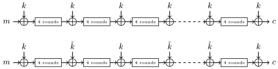
The general layout of the encryption algorithm is illustrated by the following Figure 1. It exhibits a special feature of this cipher – there is no key schedule. Key additions are effected by the function AddRoundKey (AK). It performs an

♠ ❦

✹ r♦✉♥❞s

❦

✹ r♦✉♥❞s

❦

✹ r♦✉♥❞s

❦ ❦

✹ r♦✉♥❞s

❦ ❝

♠ ❦

✹ r♦✉♥❞s

⑦❦

✹ r♦✉♥❞s

❦

✹ r♦✉♥❞s

⑦❦ ⑦❦

✹ r♦✉♥❞s

❦ ❝

Fig. 1.LEDkey usage: 64-bit key (top) and 128-bit key (bottom).

XOR. It is applied for input- and output-whitening as well as after every fourth round.

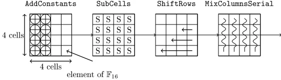
Next, Figure 2 provides an overview of the structure of one round of theLED encryption algorithm. All matrices are defined over the fieldF16.

❆❞❞❈♦♥st❛♥ts ❙✉❜❈❡❧❧s ❙❤✐❢t❘♦✇s ▼✐①❈♦❧✉♠♥s❙❡r✐❛❧

✹ ❝❡❧❧s

✹ ❝❡❧❧s

❡❧❡♠❡♥t ♦❢ ❋✶✻

❙ ❙ ❙ ❙

❙ ❙ ❙ ❙

❙ ❙ ❙ ❙

❙ ❙ ❙ ❙

Fig. 2.An overview of a single round ofLED

In the following, we construct the polynomial representation of each step. It will be contained inF2[pi, ki, x

(r) i , y

(r) i z

(r)

i , ci |i= 1, . . . ,64;r= 1, . . . ,32], a polynomial ring having no less than 6336 indeterminates.

AddConstants (AC). For every round, a round constant consisting of a tuple of six bits (b5, b4, b3, b2, b1, b0) is defined as follows. Before the first round, we start with the zero tuple. In consecutive rounds, we start with the previous round constant. Then we shift the six bits one position to the left. The new value ofb0is computed asb5+b4+ 1. This results in the round constants whose hexadecimal values are given in Table 1.

Rounds Constants

1-24 01,03,07,0F,1F,3E,3D,3B,37,2F,1E,3C,39,33,27,0E,1D,3A,35,2B,16,2C,18,30 25-48 21,02,05,0B,17,2E,1C,38,31,23,06,0D,1B,36,2D,1A,34,29,12,24,08,11,22,04

Table 1.TheLEDround constants.

Next, the round constant is divided intox=b5kb4kb3andy=b2kb1kb0 where we interpretxandyas elements of_F16. Then we form the matrix



  

0 x 0 0 1 y 0 0 2 x 0 0 3 y 0 0



  

To represent this operation by polynomials, we distinguish two cases: round number r = 1 and round numbers r > 1. In the first case we model the in-put whitening and the first application of ACin one step. Since the first round constants vector is (b5, b4, b3, b2, b1, b0) = (0,0,0,0,0,1), we get

x(1)_i =pi+ki+ 1 fori∈ {20,24,35,51,52,56},

x(1)_i =pi+ki otherwise.

Here the indeterminates x(1)_i describe the state after the first application of AC. Similarly, letx(_ir) describe the state after the r-th application ofAC, for

r = 2, . . . ,32, and let z_i(r) denote the state of the cipher after the application ofMSCin roundr.

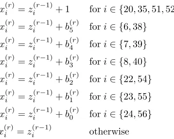
For the case r > 1, let (b(₅r), b₄(r), b(₃r), b(₂r), b₁(r), b(₀r)) be the r-th round con-stants vector, as definied in Table 1. Then we get

x(_ir)=z_i(r−1)+ 1 fori∈ {20,35,51,52}

x(_ir)=z_i(r−1)+b(₅r) fori∈ {6,38}

x(_ir)=z_i(r−1)+b(₄r) fori∈ {7,39}

x(_ir)=z_i(r−1)+b(₃r) fori∈ {8,40}

x(_ir)=z_i(r−1)+b(₂r) fori∈ {22,54}

x(_ir)=z_i(r−1)+b(₁r) fori∈ {23,55}

x(_ir)=z_i(r−1)+b(₀r) fori∈ {24,56}

x(_ir)=z(_ir−1) otherwise

in rounds whose round numberris not divisible by four, and the same equations plus a keybit addition every fourth round.

SubCells (SC). During this step, every entryxof the state matrix is replaced by the elementS(x) from the SBox given in Table 2. Letx1kx2kx3kx4be the

x 0 1 2 3 4 5 6 7 8 9 A B C D E F

S[x]C 5 6 B 9 0 A D 3 E F 8 4 7 1 2

Table 2.TheLEDSBox.

as follows.

y1=x1x2x4+x1x3x4+x2x3x4+x2x3+x1+x3+x4+ 1

y2=x1x2x4+x1x3x4+x1x3+x1x4+x3x4+x1+x2+ 1

y3=x1x2x4+x1x3x4+x2x3x4+x1x2+x1x3+x1+x3

y4=x2x3+x1+x2+x4

In our polynomial representation of theLEDencryption algorithm, this step will be combined with the next.

ShiftRows (SR). Fori = 1,2,3,4, thei-th row of the state matrix is shifted cyclically to the left by i−1 positions. Equivalently, this permutation of the 64-bit state can be described by

σ= (17 29 25 21)(18 30 26 22)(19 31 27 23)(20 32 28 24)

(33 41)(34 42)(35 43)(36 44)(37 45)(38 46)(39 47)(40 48)

(49 53 57 61)(50 54 58 62)(51 55 59 63)(52 56 60 64)

Note that the first row of the state matrix stays fixed under theShiftRows per-mutation. Thus the indices 1, . . . ,16 do not appear in the above representation ofσ.

Now we model the combined effect of SubCells and ShiftRows. Let i1 = 4i−3,i2= 4i−2,i3 = 4i−1 and i4= 4i fori= 1, . . . ,16. Then, in round r, we get the following four equations.

y(_σr₍)_i

1)=x

(r) i1 x

(r) i2 x

(r) i4 +x

(r) i1 x

(r) i3 x

(r) i4 +x

(r) i2 x

(r) i3 x

(r) i4 +

x(_ir₂)x(_i3r)+x_i(r₁)+x_i(r₃)+x(_ir₄)+ 1

y(_σr₍)_i

2)=x

(r) i1 x

(r) i2 x

(r) i4 +x

(r) i1 x

(r) i3 x

(r) i4 +x

(r) i1 x

(r) i3 +

x(_ir)

1 x

(r) i4 +x

(r) i3 x

(r) i4 +x

(r) i1 +x

(r) i2 + 1

y(_σr₍)_i

3)=x

(r) i1 x

(r) i2 x

(r) i4 +x

(r) i1 x

(r) i3 x

(r) i4 +x

(r) i2 x

(r) i3 x

(r) i4 +

x(_ir)

1 x

(r) i2 +x

(r) i1 x

(r) i3 +x

(r) i1 +x

(r) i3

y(_σr₍)_i

4)=x

(r) i2 x

(r) i3 +x

(r) i1 +x

(r) i2 +x

(r) i4

MixColumnsSerial (MCS). Every columnv of the state matrix is replaced by the productM·v, where M is the matrix

M =



  

4 1 2 2 8 6 5 6 B E A 9 2 2 F B



Let y₁(r) k · · · k y₆₄(r) be the state of the cipher after ShiftRows has been executed in roundr, and letz₁(r)k · · · kz(₆₄r)be its state afterMCS. The entries of the state matrix are the field elementsy(₄r_i−)₃x3_+y(r)

4i−2x2+y (r) 4i−1x+y

(r) 4i ofF16. Plugging these into the above matrix multiplication yields, for instance, the following first entry of the resulting state matrix.

z(₁r)x3+z(₂r)x2+z(₃r)x+z₄(r)= x2·(y(₁r)x3+y₂(r)x2+y₃(r)x+y₄(r))

+ 1·(y₁₇(r)x3+y(₁₈r)x2+y₁₉(r)x+y(₂₀r))

+ x·(y₃₃(r)x3+y₃₄(r)x2+y₃₅(r)x+y(₃₆r))

+ x·(y₄₉(r)x3+y(₅₀r)x2+y₅₁(r)x+y(₅₂r)).

After expanding, simplifying, and comparing the coefficients of 1, x, x2_{, x}3_, we finally get 64 equations

z(_jr)

1 =y

(r)

j3 +y

(r)

j5 +y

(r)

j10+y

(r)

j14

z(_jr)

2 =y

(r)

j1 +y

(r)

j4 +y

(r)

j6 +y

(r)

j11+y

(r)

j15

z(_jr)

3 =y

(r)

j1 +y

(r)

j2 +y

(r)

j7 +y

(r)

j9 +y

(r)

j12+y

(r)

j13+y

(r)

j16

z(_jr)

4 =y

(r)

j2 +y

(r)

j8 +y

(r)

j9 +y

(r)

j13

z_j(r₅)=y_j(₁r)+y_j(₄r)+y_j(r₆)+y_j(r₇)+y_j(r₉)+y(_jr₁₁)+y(_jr₁₄)+y_j(r₁₅)

z_j(r₆)=y_j(₁r)+y_j(r₂)+y_j(r₅)+y_j(₇r)+y_j(r₈)+y_j(r₉)+y(_j10r)+y(_jr₁₂)+y_j(r₁₃)+y_j(₁₅r)+y_j(r₁₆) z(jr7)=y

(r)

j2 +y

(r)

j3 +y

(r)

j6 +y

(r)

j8 +y

(r)

j9 +y

(r)

j10+y

(r)

j11+y

(r)

j14+y

(r)

j16

z(jr8)=y

(r)

j3 +y

(r)

j5 +y

(r)

j6 +y

(r)

j10+y

(r)

j12+y

(r)

j13+y

(r)

j14

z(jr9)=y

(r)

j2 +y

(r)

j4 +y

(r)

j5 +y

(r)

j6 +y

(r)

j7 +y

(r)

j8 +y

(r)

j9 +y

(r)

j10+y

(r)

j12+y

(r)

j16

z(_jr)

10 =y

(r)

j1 +y

(r)

j3 +y

(r)

j6 +y

(r)

j7 +y

(r)

j8 +y

(r)

j9 +y

(r)

j10+y

(r)

j11+y

(r)

j13

z(_jr)

11 =y

(r)

j1 +y

(r)

j2 +y

(r)

j4 +y

(r)

j7 +y

(r)

j8 +y

(r)

j9 +y

(r)

j10+y

(r)

j11+y

(r)

j12+y

(r)

j14

z(_jr)

12 =y

(r)

j1 +y

(r)

j3 +y

(r)

j4 +y

(r)

j5 +y

(r)

j6 +y

(r)

j7 +y

(r)

j9 +y

(r)

j11+y

(r)

j15+Y

(r)

j16

z(_jr)

13 =y

(r)

j2 +y

(r)

j6 +y

(r)

j10+y

(r)

j11+y

(r)

j12+y

(r)

j14+y

(r)

j16

z(_jr)

14 =y

(r)

j3 +y

(r)

j7 +y

(r)

j11+y

(r)

j12+y

(r)

j13+y

(r)

j15

z_j(₁₅r) =y_j(₁r)+y_j(₄r)+y_j(r₅)+y_j(r₈)+y_j(r₁₂)+y_j(r₁₃)+y_j(r₁₄)+y_j(r₁₆) z_j(₁₆r) =y_j(₁r)+y_j(r₅)+y_j(r₉)+y_j(r₁₀)+y_j(r₁₁)+y_j(₁₂r)+y_j(r₁₃)+y_j(r₁₅)+y_j(r₁₆)

wherei∈ {1,2,3,4}andjk= 4i−4 +k,j4+k = 4i+ 12 +k,j8+k= 4i+ 28 +k, andj12+k = 4i+ 44 +kfork= 1,2,3,4.

Final Key Addition. Fori= 1, . . . ,64, the equationsci=z (32)

3

Algebraic Representation of the Fault Equations

The algebraic representation of LED-64 constructed above is not suitable to launch a successful algebraic attack. It involves too many non-linear equations in too many indeterminates. To reconstruct the secret key from given (correct or faulty) plaintext – ciphertext pairs requires additional information. This in-formation will be furnished by a fault attack. In [12] we discussed a method for injecting fault and using it to break LED-64 by exhaustive search. In the following, we construct a polynomial version of the fault equations which were generated there.

Let us recall the description of the attack. We assume the following fault model. The attacker is supposed to be able to encrypt the same plain text unit twice using the same secret keyk. The first encryption takes place correctly, and during the second encryption a fault is introduced. The fault is a random change in the value of the first (4-bit sized) entry of the state matrix at the beginning of round 30. As a consequence, we obtain a correct ciphertext c and a faulty ciphertextc0.

The propagation of the fault is observed. It leads to an incorrect first column of the state matrix after the SBox has been applied in round 31 whose 4-bit entries we denote bya, b, c, d. In [12] we derived the following 16 fault equations fora, b, c, d.

a=D·(S−1(C·(¯c1+ ¯k1) +C·(¯c5+ ¯k5) +D·(¯c9+ ¯k9) +4·(¯c13+ ¯k13)) +

S−1(C·(¯c01+ ¯k1) +C·(¯c05+ ¯k5) +D·(¯c09+ ¯k9) +4·(¯c013+ ¯k13))) (Ea,0)

a=F·(S−1(3·(¯c4+ ¯k4) +8·(¯c8+ ¯k8) +4·(¯c12+ ¯k12) +5·(¯c16+ ¯k16)) +

S−1(3·(¯c04+ ¯k4) +8·(¯c08+ ¯k8) +4·(¯c012+ ¯k12) +5·(¯c016+ ¯k16))) (Ea,1)

a=5·(S−1(7·(¯c3+ ¯k3) +6·(¯c7+ ¯k7) +2·(¯c11+ ¯k11) +E·(¯c15+ ¯k15)) +

S−1(7·(¯c30 + ¯k3) +6·(¯c

0

7+ ¯k7) +2·(¯c

0

11+ ¯k11) +E·(¯c

0

15+ ¯k15))) (Ea,2)

a=9·(S−1(D·(¯c2+ ¯k2) +9·(¯c6+ ¯k6) +9·(¯c10+ ¯k10) +D·(¯c14+ ¯k14)) +

S−1(D·(¯c20 + ¯k2) +9·(¯c

0

6+ ¯k6) +9·(¯c

0

10+ ¯k10) +D·(¯c

0

14+ ¯k14))) (Ea,3)

b=1·(S−1(C·(¯c4+ ¯k4) +C·(¯c8+ ¯k8) +D·(¯c12+ ¯k12) +4·(¯c16+ ¯k16)) +

S−1(C·(¯c40 + ¯k4) +C·(¯c

0

8+ ¯k8) +D·(¯c

0

12+ ¯k12) +4·(¯c

0

16+ ¯k16))) (Eb,0)

b=7·(S−1(3·(¯c3+ ¯k3) +8·(¯c7+ ¯k7) +4·(¯c11+ ¯k11) +5·(¯c15+ ¯k15)) +

S−1(3·(¯c03+ ¯k3) +8·(¯c07+ ¯k7) +4·(¯c011+ ¯k11) +5·(¯c015+ ¯k15))) (Eb,1)

b=3·(S−1(7·(¯c2+ ¯k2) +6·(¯c6+ ¯k6) +2·(¯c10+ ¯k10) +E·(¯c14+ ¯k14)) +

S−1(7·(¯c02+ ¯k2) +6·(¯c06+ ¯k6) +2·(¯c010+ ¯k10) +E·(¯c014+ ¯k14))) (Eb,2)

b=9·(S−1(D·(¯c1+ ¯k1) +9·(¯c5+ ¯k5) +9·(¯c9+ ¯k9) +D·(¯c13+ ¯k13)) +

S−1(D·(¯c10 + ¯k1) +9·(¯c

0

5+ ¯k5) +9·(¯c

0

9+ ¯k9) +D·(¯c

0

c=9·(S−1(C·(¯c3+ ¯k3) +C·(¯c7+ ¯k7) +D·(¯c11+ ¯k11) +4·(¯c15+ ¯k15)) +

S−1(C·(¯c30 + ¯k3) +C·(¯c

0

7+ ¯k7) +D·(¯c

0

11+ ¯k11) +4·(¯c

0

15+ ¯k15))) (Ec,0)

c=B·(S−1(3·(¯c2+ ¯k2) +8·(¯c6+ ¯k6) +4·(¯c10+ ¯k10) +5·(¯c14+ ¯k14)) +

S−1(3·(¯c02+ ¯k2) +8·(¯c06+ ¯k6) +4·(¯c010+ ¯k10) +5·(¯c014+ ¯k14))) (Ec,1)

c=C·(S−1(7·(¯c1+ ¯k1) +6·(¯c5+ ¯k5) +2·(¯c9+ ¯k9) +E·(¯c13+ ¯k13)) +

S−1(7·(¯c01+ ¯k1) +6·(¯c05+ ¯k5) +2·(¯c09+ ¯k9) +E·(¯c013+ ¯k13))) (Ec,2)

c=8·(S−1(D·(¯c4+ ¯k4) +9·(¯c8+ ¯k8) +9·(¯c12+ ¯k12) +D·(¯c16+ ¯k16)) +

S−1(D·(¯c40 + ¯k4) +9·(¯c

0

8+ ¯k8) +9·(¯c

0

12+ ¯k12) +D·(¯c

0

16+ ¯k16))) (Ec,3)

d=9·(S−1(C·(¯c2+ ¯k2) +C·(¯c6+ ¯k6) +D·(¯c10+ ¯k10) +4·(¯c14+ ¯k14)) +

S−1(C·(¯c20 + ¯k2) +C·(¯c

0

6+ ¯k6) +D·(¯c

0

10+ ¯k10) +4·(¯c

0

14+ ¯k14))) (Ed,0)

d=7·(S−1(3·(¯c1+ ¯k1) +8·(¯c5+ ¯k5) +4·(¯c9+ ¯k9) +5·(¯c13+ ¯k13)) +

S−1(3·(¯c10 + ¯k1) +8·(¯c

0

5+ ¯k5) +4·(¯c

0

9+ ¯k9) +5·(¯c

0

13+ ¯k13))) (Ed,1)

d=2·(S−1(7·(¯c4+ ¯k4) +6·(¯c8+ ¯k8) +2·(¯c12+ ¯k12) +E·(¯c16+ ¯k16)) +

S−1(7·(¯c04+ ¯k4) +6·(¯c08+ ¯k8) +2·(¯c012+ ¯k12) +E·(¯c016+ ¯k16))) (Ed,2)

d=5·(S−1(D·(¯c3+ ¯k3) +9·(¯c7+ ¯k7) +9·(¯c11+ ¯k11) +D·(¯c15+ ¯k15)) +

S−1(D·(¯c03+ ¯k3) +9·(¯c07+ ¯k7) +9·(¯c011+ ¯k11) +D·(¯c015+ ¯k15))) (Ed,3)

In these equations, the indeterminates ¯k1, . . . ,k¯16 represent the 4-bit parts of the secret key, the indeterminates ¯c1, . . . ,¯c16 represent the parts of the cor-rect ciphertext, and ¯c0₁, . . . ,c¯0₁₆ the parts of the faulty ciphertext. Since these equations involve the map S−1 _:

F16 −→ F16, we need to find a polynomial representation of this map. Using the values of this map given in Table 3 and

x 0 1 2 3 4 5 6 7 8 9 A B C D E F

S−1_{(x)5 E F 8 C 1 2 D B 4 6 3 0 7 9 A}

Table 3.The inverseLEDSBox.

univariate interpolation, we construct the following polynomial representation ofS−1_.

S−1(y) = (x2+ 1) + (x2+ 1)y+ (x3+x)y2+ (x3+x2+ 1)y3+xy4+ (x3+ 1)y5+ (x3+ 1)y7+ (x+ 1)y9+ (x2+ 1)y10+ (x3+ 1)y11+

Next, we plug the right-hand sides of the fault equations into this polynomial. We get 16 polynomial fault equations which are defined over the polynomial ring_F16[a, b, c, d,¯k1, . . . ,¯k16,¯c1, . . . ,¯c16,¯c01, . . . ,c¯016]. For every group of equations

Et,0, Et,1, Et,2, Et,3 having the same left-hand side t ∈ {a, b, c, d}, we can form three differences Et,0−Et,i = 0 with i = 1,2,3. Now, comparing coefficients for{1, x, x2_{, x}3_{}yields 48 equations in the bitsk}

1, . . . , k64of the secret key, the bits c1, . . . , c64 of the correct ciphertext, and the bits c01, . . . , c064 of the faulty ciphertext. Notice that we can use the field equationsk2

i +ki= 0, c2i +ci = 0, and (c0_i)2+c0_i= 0 for simplification here.

Altogether, we find 48 polynomials inF2[k1, . . . , k64, c1, . . . , c64, c01, . . . , c064]. They all have degree 3 and consist of approximately 3400-8800 terms. These polynomials will be called thefault polynomials.

4

An Algebraic Fault Attack on

LED-64

4.1 Description of the Attack

In the preceding two sections we derived polynomials describing the encryption map of LED-64 and additional information gained from a fault attack. All in all, we found 6208 polynomials in 6336 indeterminates describing the encryption map, 6336 field equations, and 48 fault polynomials in 192 indeterminates.

As mentioned previously, we assume that we are able to mount a known-plaintext-attack and a repeat encryption involving the same key and the fault injection described previously. For every concrete instance of this attack, we can therefore substitute the plaintext bits, correct ciphertext bits, and faulty cipher-text bits into our polynomials. After this substitution, we have 6208 polynomials in 6208 indeterminates for the encryption map, 6208 field equations, and 48 fault polynomials in the 64 indeterminates of the secret key.

The resulting fault polynomials consist typically of 40-150 terms. Some of them (usually no more than 5) drop their degree and become linear. Of course, these linear polynomials are particularly valuable, since they decrease the com-plexity of the problem by one dimension. In the experiments reported below it turned out to be beneficial to interreduce the fault polynomials after substitution in order to generate more linear ones.

The polynomial systems can be solved using various techniques. For our experiments, we applied the algorithms for conversion to a SAT-solving problem explained in [11].

4.2 Experimental Results

SAT solver MS(1 thread)CMS(1 thread)CMS(4 threads)

time (in sec) 90852 71656 22639

time (in h) 25.23 19.90 6.28

Table 4.Average SAT Solver Timings.

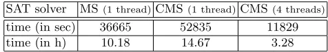
For the second set of experiments, we first interreduced the fault polynomials using the computer algebra systemApCoCoA(see [1]) and then appended the linear polynomials to the system. In this way we were sometimes able to find more linear dependencies between the key indeterminates, thereby reducing the dimension even further. Moreover, the SAT-solvers appear to benefit from this simplification, because it is typically the number of terms in a polynomial that complicates its logical representation. This seemingly minor modification results in a meaningful speed-up, as we can see in Table 5.

SAT solver MS(1 thread)CMS(1 thread)CMS(4 threads)

time (in sec) 36665 52835 11829

time (in h) 10.18 14.67 3.28

Table 5.Average SAT Solver Timings with Additional Linear Equations.

In summary, it is clear that the proposed attack is able to break theLED-64 encryption scheme. While it is slower than the direct fault attack presented in [12], it does not rely on the specific properties underlying the key filtering steps there, and it offers numerous possibilities for optimization.

5

Conclusions and Future Work

After providing a complete algebraic description of the LED block cipher and showing how to convert the previously introduced fault equations into fault polynomials, it turned out that the combined polynomial system was solvable by state-of-the-art SAT solvers. Therefore the idea of combining an algebraic attack on a block cipher with fault-injection cryptanalysis is able to break the LED-64encryption algorithm in practice. This demonstrates that analysing the results of fault injection by algebraic methods is a promising approach. It may make it possible to attack ciphers for which the polynomial system resulting from a purely algebraic attack could not be solved in a reasonable time previously.

methods to more challenging encryption schemes such as LED-128or PRESENT. Furthermore, we plan to generalize the attack to other kinds of block ciphers, e.g. to Feistel network block ciphers such asDES, and to public key encryption schemes.

Acknowledgements. The authors are grateful to Mate Soos for numerous discussions and valuable information about the program CryptoMiniSat, about SAT-solving in general, and for being always ready to help with solver-related problems.

References

1. ApCoCoA: Applied Computations in Commutative Algebra, available for download athttp://www.apcocoa.org.

2. H. Bar-El, H. Choukri, D. Naccache, M. Tunstall, C. Whelan, The Sorcerer’s Ap-prentice Guide to Fault Attacks, Proceedings of the IEEE, vol.94, IEEE Computer Society, 2006, pp. 370–382.

3. E. Biham ans O. Dunkelman, Techniques for cryptanalysis of block ciphers, Springer, Heidelberg 2011.

4. A. Bogdanov, L.R. Knudsen, G. Leander, C. Paar, A. Poschmann, M.J.B. Rob-shaw, Y. Seurin and C. Vikkelsoe, PRESENT: An Ultra-Lightweight Block Cipher, In: P. Paillier and I. Verbauwhede (eds.) CHES2007, LNCS, vol.4727, Springer, Heidelberg 2007, pp. 450–466.

5. D. Boneh, R.A. DeMillo and R.J. Lipton, On the Importance of Elimination Errors in Cryptographic Computations, J. Cryptology14(2001), 101–119.

6. C. Carlet, J-C. Faugere, C. Goyet, G. Renault, Analysis of the algebraic side channel attack, Journal of Cryptographic Engineering, vol.2nr. 1, Springer Heidelberg 2012, pp. 45–62.

7. J. Guo, T. Peyrin, A. Poschmann and M. Robshaw, The LED Block Cipher, In: B. Preneel and T. Takagi (eds.)CHES 2011, LNCS, vol. 6917, Springer, Heidelberg 2011, pp. 326–341.

8. D. Hong, J. Sung, S. Hong, J. Lim, S. Lee, B. Koo, C. Lee, D. Chang, J. Lee, K. Jeong, H. Kim, J. Kim, S. Chee, HIGHT: A New Block Cipher Suitable for Low-Resource Device, In: L. Goubin and M. Matsui (eds.)CHES2006, LNCS, vol.4249, Springer, Heidelberg 2006, pp. 46–59.

9. M. Hojs´ık and B. Rudolf, Differential Fault Analysis of Trivium, In: K. Nyberg (ed.)

FSE2008, LNCS, vol.5086, Springer, Heidelberg 2008, pp. 158–172.

10. M. Hojs´ık and B. Rudolf, Floating Fault Analysis of Trivium, In: D.R. Chowd-hury, V. Rijmen and A. Das (eds.)INDOCRYPT2008, LNCS, vol.5365, Springer, Heidelberg 2008, pp. 239–250.

11. P. Jovanovic and M. Kreuzer, Algebraic Attacks using SAT-Solvers, Groups – Complexity – Cryptology2(2010), pp. 247–259.

12. P. Jovanovic, M. Kreuzer, I. Polian, A Fault Attack on the LED Block Cipher, In: W. Schindler and S. Huss (eds.) COSADE 2012, LNCS, vol. 7275, Springer Heidelberg 2012, pp. 120–134.

14. M. Kreuzer and L. Robbiano, Computational Commutative Algebra 1, Springer Verlag, Heidelberg 2000.

15. M.S.E. Mohamed, S. Bulygin and J. Buchmann, Using SAT Solving to Improve Differential Fault Analysis of Trivium, In: T-H. Kim, H. Adeli, R.J. Robles and M.O. Balitanas (eds.) ISA 2011, CCIS, vol. 200, Springer, Heidelberg 2011, pp. 62–71.

16. D. Mukhopadhyay, An Improved Fault Based Attack of the Advanced Encryption Standard, In: B. Preneel (ed.) AFRICACRYPT2009, LNCS, vol.5580, Springer, Heidelberg 2009, pp. 421–434.

17. National Institute of Standards and Technology (NIST). Advanced Encryption Standard (AES). FIPS Publication 197, available for download at

http://www.itl.nist.gov/fipsbups/, 2001.

18. M. Renauld, F-X. Standaert and N. Veyrat-Charvillon, Algebraic Side-Channel Attacks on the AES: Why Time also Matters in DPA, In: C. Clavier and K. Gaj (eds.)CHES2009, LNCS, vol.5747, Springer Heidelberg 2009, pp. 97–111. 19. M. Tunstall, D. Mukhopadhyay and S. Ali, Differential Fault Analysis of the