R E S E A R C H
Open Access
Cross-layer design for decentralized detection
in WSNs
Ashraf Tantawy
1*, Xenofon Koutsoukos
2and Gautam Biswas
2Abstract
A wireless sensor network (WSN) deployed for detection applications has the distinguishing feature that the sensors cooperate to perform the detection task. Therefore, the decoupled and maximum throughput design approaches typically used to design communication networks do not lead to the desired optimal detection performance. Recent work on decentralized detection has addressed the design of media access control (MAC) and routing protocols for detection applications by considering independently the quality of information (QoI), channel state information (CSI), and residual energy information (REI) for each sensor. However, little attention has been given to integrate the three quality measures (QoI, CSI, and REI) in the system design. In this work, we present a cross-layer approach to design a QoI, CSI, and REI-aware transmission control policy (XCP) that coordinates communication between local sensors and the fusion center, in order to maximize the detection performance. We formulate and solve a constrained non-linear optimization problem to find the optimal XCP design variables, for both ALOHA and time-division multiple access (TDMA) sensor networks. We show the detection performance gain compared to the typical decoupled and maximum throughput design approaches, without utilizing additional network resources. We compare ALOHA and TDMA MAC schemes and show the conditions under which each transmission scheme outperforms.
Keywords: Decentralized detection; Wireless sensor networks; Networked information fusion; Multiaccess communication
1 Introduction
The deployment of wireless sensor networks (WSNs) in decentralized detection applications is motivated by the availability of low-cost sensors with computational capabilities, combined with advances in communication network technologies. In decentralized detection (DD), multiple sensors collaborate to distinguish between two or more hypotheses, and the classical problem is to find the local sensor detection strategies (quantization rules) to minimize a system-wide cost function using differ-ent network topologies and channel models [1,2]. Despite the fact that this classical problem is insightful, current research on detection using modern WSNs has shifted the focus away from this classical quantization problem for two main reasons: (1) performance loss due to quantiza-tion decays rapidly with the number of informaquantiza-tion bits in the packet payload [3,4], and (2) the payload of a packet could be considered large enough to represent local sensor
*Correspondence: [email protected]
1Global Operations Organization, British Petroleum Egypt, Cairo 11728, Egypt Full list of author information is available at the end of the article
information with adequate accuracy, as additional bits in the payload are unlikely to affect power or delay, given the relatively large packet overhead [5,6] (e.g., IEEE 802.15.4 standard has a minimum of 9 bytes for the medium access control (MAC) overhead [7]). On the other hand, the deployment of WSNs in detection applications brings new challenges to the field. In addition to the design of sig-nal processing algorithms at the application layer that has been previously addressed [8], protocols for other com-munication layers have to be optimized to maximize the detection performance.
The layered approach commonly adopted to design wireless networks may not be appropriate for detec-tion applicadetec-tions. Although the layered approach provides simplicity in the design due to the decoupling of sys-tem layers, it neither provides the optimal resource allo-cation nor exploits the appliallo-cation domain knowledge. As an example, throughput is a common performance metric used to design media access control protocols. In DD applications, maximizing the throughput is not the prime objective, rather maximizing the quality of
the information received that yields the best detection performance is the prime objective. Accordingly, a cross-layer design approach is desired for efficient implementa-tion of WSNs in decentralized detecimplementa-tion applicaimplementa-tions.
In this paper, we pursue a cross-layer approach to design a WSN deployed for detection applications. We integrate the physical, MAC, and detection application layers in one unified model that captures different sensor quality mea-sures. In making our modeling choices, we are motivated by the desire to develop a system model that captures the basic features of practical sensor networks while being amenable to analysis. Specifically, we make the following design assumptions:
1. Digital transmission. Although uncoded analog transmission is optimal in a sensor network under certain conditions (see, e.g., [9]), digital transmission is still the choice for cost-effective, commercial off-the-shelf deployments of sensor network applications.
2. Slotted ALOHA/time-division multiple access (TDMA) MAC. The traditional assumption of a dedicated orthogonal channel between each sensor node and the fusion center may not be feasible in practice. On the other hand, random access techniques and TDMA are frequently used MAC protocols. Therefore, tuning of the protocol parameters to optimize the detection performance can be done in practice without a need to redesign the system.
3. Single hop networks. We focus on the case where sensor nodes cannot communicate with each other to form a multihop network to the fusion center, e.g., radio-frequency identification (RFID) sensors communicating to an RFID reader. Preliminary results for multihop tree networks are presented in [10,11].
The rest of the paper is organized as follows: Section 2 summarizes the related work. Section 3 presents the detection problem formulation for WSNs. Section 4 explains the derivation of the system model. Section 5 presents the solution of the optimization problem. Section 6 presents the performance comparison between the proposed design approach and the classical design approaches. Section 7 presents a performance comparison between the TDMA and ALOHA networks. The work is concluded in Section 8.
2 Related work
Early work on cross-layer design has focused on the design of channel-aware decentralized detection schemes [12]. More recent work on channel-aware design considers sequential detection schemes [13]. The cross-layer design approach has been recently explored for the design of
MAC and routing protocols for detection applications. Cooperative MAC, where individual sensor transmissions are superimposed in a way that allows the fusion center to extract the relevant detection information, is considered in [14]. This approach leads to significant gains in per-formance when compared to conventional architectures allocating different orthogonal channels for each sen-sor. However, technical issues such as symbol and phase synchronization have to be taken into account for prac-tical implementations [5,15]. Data-centric MAC, where existing protocols are tuned/modified for optimal perfor-mance, represents a viable alternative to cooperative MAC and, therefore, has gained considerable attention recently. Decision fusion over slotted ALOHA MAC employing a collision resolution algorithm is studied in [16], where the objective is to analyze the performance, rather than to design the MAC layer, in order to optimize the detection performance. A more thorough investigation of the design of MAC transmission policies to minimize the error prob-ability has been considered in [17], where the system model includes the MAC and detection application lay-ers, excluding the physical channel model, and assuming a stochastic MAC policy. Although stochastic transmis-sion policy results in performance gains compared to deterministic policies, the extension of this framework to include the physical channel model is challenging mathe-matically.
The integration of the channel model and the MAC layer in the context of distributed estimation has been considered in [18], where analog transmission of sensor data is assumed. The cross-layer approach is also consid-ered in [6], where an integrated model for the physical channel and the queuing behavior for sensors is devel-oped. The design problem is to choose the code rate and the number of sensors to minimize the error probability for an frequency-division multiple access (FDMA) system, where orthogonal channels are used between sensors and the fusion center.
Routing for decentralized detection has been consid-ered separately from the MAC design problem. Energy-efficient routing for signal detection in WSNs is consid-ered in [19], where the objective is to find the optimal route for local data from a target location to the fusion center. Cooperative routing for distributed detection in large sensor networks is studied in [20] using a link met-ric that characterizes the detection error exponent. For a survey on the interplay between signal processing and net-working in sensor networks, see [21] and the references therein.
We summarize the contributions of this paper, as com-pared to existing literature, in the following main points:
detection application layer in one unified system model.
2. Integration of different sensor quality measures. The model captures three sensor quality measures, namely, quality of information (QoI), channel state information (CSI), and residual energy information (REI). In addition, delay for detection and network lifetime are considered as additional design constraints.
3. Design of a complete transmission control policy. We design an optimal transmission control policy that includes not only the transmission probabilities but also the communication rate and the energy allocation for each sensor. The authors are not aware of a literature work on cross-layer design for
detection applications, where an integrated model is developed that captures different communication layers and several sensor quality measures, while simultaneously considering different transmission design parameters as well as the delay for detection. 4. Non-asymptotic analysis. We assume a finite number
of sensor nodes and do not resort to asymptotic analysis as commonly adopted in detection studies. Therefore, the analysis results are applicable on small-scale and large-scale sensor networks.
5. Enhanced detection performance. Without
additional resources, the proposed design approach outperforms the classical decoupled and maximum throughput design approaches.
6. Slotted ALOHA-TDMA comparative analysis. We
show the conditions under which each transmission scheme outperforms. These conditions represent a guideline for the designer to choose between the two protocols based on the available system resources and design constraints.
The work presented in this paper is an extension of our previous work in [22], where only ALOHA networks were considered, and the energy allocation scheme was fixed. In addition, a more detailed simulation experiment and
a full comparison between ALOHA and TDMA sensor networks are presented.
3 Problem formulation
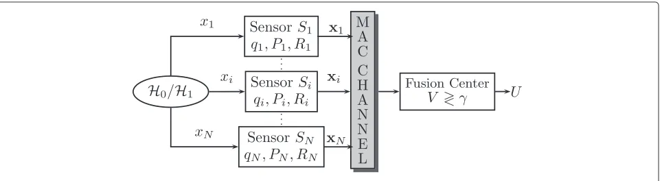
Figure 1 illustrates the detection system architecture, where a set ofN wireless sensors,S = {S1,S2,. . .,SN}, and a fusion center (FC) collaborate to detect the phe-nomenon of interest in a geographic area divided into a number of resolution cells. We can summarize our design problem as “Given the CSI, REI, and QoI for each sensor, how can we find the optimal transmission control policy (XCP) for each sensor that maximizes the system detection performance?”
Initially, the fusion center broadcasts a message con-taining the location of the resolution cell to be surveyed, soliciting information from different sensors. Each sensor responds with the following information: (1) channel state between the sensor and the fusion center, which could be estimated using channel measurement techniques [23,24]; (2) signal-to-noise ratio for the reflected probing signal used by the sensor to illuminate the target, which could be estimated from sensor location (estimated using dif-ferent localization methods [25]), resolution cell location, and channel measurement techniques; and (3) the energy reserve, representing the REI, which could be estimated by the sensor from the battery charging state. We call this communication process the handshaking cycle, which starts with the broadcast message from the fusion center and ends when the fusion center receives the informa-tion from all sensors. This handshaking cycle is repeated periodically to cope with changes in the environment that impact the sensor quality measures. Therefore, the overhead of the handshaking cycle is proportional to the environment dynamics, i.e., how fast the environment changes to affect the quality measures for sensors. We ignore the handshaking overhead in the development of the system model in Section 4. In Section 4.6, we provide an upper bound on the environment dynamics such that the handshaking overhead could be safely ignored without affecting the model accuracy.
After the handshaking cycle, the fusion center calculates the optimal transmission control policy for each sensor based on the quality measures received. The values of the XCP variables are then sent back to the sensors that have reliable quality measures to contribute to the detec-tion task. The resulting values of the XCP variables are stored in a lookup table in the sensor memory (for each resolution cell), which remain valid for the given location as long as the quality measures for each sensor have not changed from the last run of the optimization algorithm. The detection process then proceeds as follows: the fusion center broadcasts a message to initiate a detection cycle for a specific resolution cell. The local sensors selected by the optimization algorithm will sample the environment by collecting a number of observations xi, form a data packet, and communicate their messages directly to the fusion center over the MAC channel. Finally, the fusion center makes a final decision after a fixed amount of time representing the maximum allowed delay for detection.
4 System model
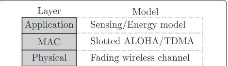
The detection scheme described above suggests a layered approach to system modeling, as depicted in Figure 2. The physical layer represents the wireless channel model and defines system parameters such as the communication bit rate as well as the energy consumed in communicat-ing sensor information to the fusion center. The media access control layer represents either the slotted ALOHA or the TDMA protocol model and defines the protocol-specific parameters such as the transmission probability. Finally, the application layer represents the sensing and energy models and defines the model of the observations obtained by local sensors, as well as the WSN energy con-straints. In what follows, we derive the model for each layer of the system.
4.1 Wireless channel model
We focus on the case where the sensor nodes and the fusion center have minimal movement and the environ-ment changes slowly. Accordingly, only the slow-fading component of the wireless channel is considered. Figure 3 shows the fading channel model, wherew(t)is an AWGN with PSDN0/2, andm(dc)is the mean path attenuation
for a sensor node at a distancedcfrom the fusion center.
Figure 2A layered approach to detection system modeling.
Using the Hata path-loss model, the total decibel power loss is given by [26]
PL=20 log
4πd0/λp
+10ρclog(dc/d0)
μc
+Xσc dB
(1)
whered0is a reference distance corresponding to a point
located in the far field of the transmit antenna,λpis the wavelength of the propagating signal,ρc is the path loss
exponent, andXσc ∼N(0,σc2).
The wireless channel represents an unreliable bit pipe for the data link layer, with instantaneous Shannon capac-ityC= Wlog2(1+Pr/N0W)bps, whereW is the
chan-nel bandwidth and Pr is the signal power received by
the fusion center. Using Shannon’s coding theorem and given the state-of-the-art coding schemes that approach the Shannon capacity, we can approximately assume that the fusion center can perform error-free decoding for any transmission with bit rateR<C, i.e., the channel is con-sidered ‘ON’ when R < C and ‘OFF’ otherwise, giving rise to the two-state channel model akin to [6]. Using (1), the probability of the channel being ON during sensori
transmission could be expressed as
λi
c=
1 σi
c
10 log P
i
t
N0W(2Ri/W−1) −μ
i
c
, (2)
wherePtis the average transmitted signal power, and(.)
is the cumulative distribution function for the standard normal PDF. We note that the CSI relevant to our model is represented by the statisticsσc,μc, andN0. These
statis-tics are required to be estimated by each sensor, and no instantaneous channel state information is required for the XCP design. Since we assume fixed nodes and a slowly varying channel, the estimation process could be executed less frequently to save sensor node resources. This is par-ticularly important in wireless sensor networks since the estimation of the channel state is both time and power consuming.
It should be highlighted that the large-scale fading model presented here allows us to obtain the closed form solution in (2). More complex fading models, e.g., small-scale fading, can be integrated similarly, but they may allow only numerical solutions.
4.2 Media access control protocol model
The detection cycle initiated by the fusion center is illus-trated in Figure 4. We assume a slotted multiaccess com-munication scheme with number of comcom-munication slots
Figure 3Block diagram for the wireless communication channel.
transmission over the wireless channel, with communica-tion rate:
Ri=bLni/τ, (3)
wherebis the number of encoding bits for each observa-tion. The sensorithen attempts to transmit to the fusion center according to the MAC scheme:
1. Slotted ALOHA. Sensor attempts transmission in every slot during the detection cycle, with probabilityqi, despite the state of their last transmission.
2. TDMA. Sensor transmits to the fusion center only in its dedicated time slot, assigned using the fixed assignment TDMA scheme.
Unequal priority TDMA, where a single sensor may be assigned more than one time slot, could also be used and may lead to a better detection performance. How-ever, the resulting optimization problem is an integer programming problem that is generally hard to solve in real time. Therefore, only equal-priority TDMA is consid-ered in this work. Without loss of generality, we assume thatL = mN, wheremis a positive integer, i.e., at each detection cycle, all sensors transmit the same number of times. This assumption facilitates the comparison with the slotted ALOHA scheme. The decision takes place at the end of the detection cycle by the FC. The process repeats for every detection request initiated by the fusion center. To simplify the analysis, the MAC protocol does not consider the acknowledgement slots and any protocol specifics required for synchronization or rate negotiation. Also, we ignored the packet overhead, which is a rea-sonable approximation for practical WSN protocols with large packet payload.
Now, we calculate the overall probability of a successful packet transmission:
1. Slotted ALOHA. At any given time slot, the probability of a successful packet transmission by sensori is given byqij=i(1−qj). Further, this packet will be successfully received by the fusion center if the state of the physical channel between the sensor and the fusion center is ON during this time slot.
2. TDMA. Since collisions are eliminated, the probability of successful packet transmission depends solely on the physical channel condition, as given by (2).
The total probability of a successful packet transmission by sensoriis then given by
λi=
qij=i(1−qj)
λi
c ALOHA
λi
c TDMA
(4)
4.3 Energy model
To formulate the energy model for each sensor, we first define the sensor network lifetime. Different definitions exist in the literature [27,28], and the choice of a specific definition is usually governed by the application and the tractability of the resulting problem formulation. A gen-eral definition for network lifetime is presented in [29]. The definition holds regardless of the underlying net-work model, including netnet-work architecture and protocol, channel fading characteristics, and energy consumption model. The lifetime is given by
L=E0−Ew/f
rEr=
N
i=1
(e0i −ewi) fr N
i=1 eri ,
(5)
whereE0 = Ni=1e0i is the total initial energy in all sen-sors at the time of deployment,Ew=Ni=1ewi is the total wasted energy remaining in sensor nodes when the net-work dies,fr is the average sensor reporting rate defined here as the number of detection cycles per unit time, and
Er =N
i=1eri is the expected reporting energy consumed by all sensors in one detection cycle.
Our objective is to allocate the reporting energyeri for each sensor in such a way that maximizes the detec-tion performance. In what follows, we derive the energy constraints for the sensor network.
4.3.1 Total energy constraint
In practice, it is desired to have a minimum network life-time, where sensors can perform the assigned task, i.e., L≥lt. Using (5), we get:
Er≤E0−Ew/f
rlt=
N
i=1
(e0i −ewi )
frlt=εt.
(6)
The total energy constraint is thus expressed as
N
i=1
eri ≤εt. (7)
4.3.2 Individual energy constraints
Since the network lifetime tends towards the least lifetime of sensor nodes, it is desired to keep a minimum lifetime for each sensor. This prolongs the network lifetime and avoids depleting the energy reserve for high-quality sen-sors, resulting in a quick expiry of the sensor network. In addition, depleting sensor energy may result in loss of coverage for the area under surveillance. Therefore, we impose the constraintLi ≥l,i=1, 2,. . .,Non all sensor nodes. Accordingly, we get:
eri ≤e0i −eiw/frl=εi, (8)
where we note that l < lt, i.e., εt < Ni=1εi. Other-wise, each sensor trivially allocates its maximum energyεi. Obviously, the reporting energy≥0; hence, the individual energy constraint is summarized as
0≤eri ≤εi i=1, 2,. . .,N. (9)
The constraint (9) essentially limits the energy expended by each sensor in each detection cycle to avoid fast deple-tion of the sensor energy. Finally, we need to relate the transmission powerPtin (2) to the reporting energyerin
each detection cycle. We note thatPit= eri/T, whereTis the total time the sensor is transmitting during a detection cycle.
1. ALOHA : We note that the expected number of
transmissions by sensori during a detection cycle is
Lqi. Therefore,T=(τ/L)Lqi=τqi, and we get
Pit=eri/τqi.
2. TDMA : Since we assumeL=mN, each sensor
transmitsm times, and we getPit=Neri/τ.
The total probability of successful packet transmission is then expressed as
λi=
qij=i(1−qj)
(ρi) ALOHA
(ρi) TDMA,
(10)
ρi=
ai+
10/σcilogeriqi(2Ri/W−1)
ALOHA
ai+
10/σi
c
logeriN(2Ri/W−1) TDMA,
(11)
ai= −
1/σci 10 log(N0Wτ)+μic
. (12)
We note that in the above discussion, we neglected the energy consumed by each sensor to report its quality mea-sures to the fusion center. This energy component could be included in the analysis by subtracting it from the initial sensor energy. However, for slowly varying environments, where the sensor characteristics need to be updated less frequently, this energy component could be neglected compared to the periodic sensor reporting energy.
4.4 Sensing model
We focus our work on detection using signal amplitude measurements. Therefore, the observation at sensor i, located at distancedi from an object at a specific resolu-tion cell, could be expressed as
xi= /dη/i 2+wi, (13)
where is the amplitude of the emitted signal at the object, ηis a known attenuation coefficient, typically between 2 and 4, andwiis an additive white Gaussian noise with zero mean and varianceσsi2. We note that the above model con-siders passive sensing [25]. In the active sensing case, the observation model is given byxi = ζ tr/(2di)η/2+ wi, where ζ is a known reflection coefficient at the object, tris the amplitude of the signal transmitted by the active sensor (illuminating signal), and 2di is the round trip distance traveled by the signal [19]. We note that the two observation models differ only in the scaling factor ζ/2η/2. Therefore, without loss of generality, we assume
the active sensing model in the following discussion. If passive sensing is assumed, then the detection problem will be slightly different than the problem presented here, since the amplitude of the source signal, , is unknown and has to be estimated from sensor observations.
The detection problem could be defined as the following binary hypothesis testing problem, for each time slotk:
H0:xi[j,k]=wi[j,k] j=1, 2,. . .,ni
H1:xi[j,k]=μi+wi[j,k] j=1, 2,. . .,ni, (14)
obtained by sensoriat each time slot. We note that noise samples are independent across sensors, i.e., the obser-vations at local sensors are independent across time and space, but not necessarily identically distributed since some sensors may be closer to the resolution cell, and noise variances are assumed unequal. In the following, we designate the vector of sensor observations at time slot k by xi[k]= [xi[1,k] xi[2,k] . . . xi[ni,k] ]. We note that xi[k] has the multivariate Gaussian distribu-tion N(0,C) under hypothesis H0 and N(μ,C) under
Proposition 1. The optimal test statistic at the fusion
center is given by
V =
Bernoulli random process representing the success (ri =1)
or failure (ri = 0) of receiving a packet from sensor i in
communication slot k. The sample space and probability measure of riare defined asri = {0, 1}and P[ri = 1]=
λi, respectively, whereλiis given by (4).
Proof.At the fusion center, the log likelihood ratio (LLR) is the sum of the individual observations received at each time slot. Therefore, the test could be expressed as
ns number of times sensor i successfully transmitted to the fusion center in ns time slots. The random vector z = [z1 z2 . . . zN ze], where ze = ns − Ni=1zi, is multinomially distributed with probability vector p =
[λ1 λ2 . . . λN λe], where the probability of collision or idle slot λe = 1 −
N
i=1λi, and the sample space Z represents all possible combinations ofzisuch thatze+
N
4.5 Measurement of detection performance
One of the widely used performance measures for detec-tion applicadetec-tions is the receiver operating characteristics (ROC) curve [30]. The curve relates the probability of detection PD to the probability of false alarm PFA for
different threshold values γ of the detector. For exam-ple, for the centralized shift-in-mean Gaussian detection problem, where all observations are available at the fusion center, the ROC curve is expressed as
PD=Q Q−1(PFA)− μ1−σ μ0
, (19)
whereQ[ .]= 1−[ .] is the complementary cumulative distribution function for the standard normal PDF,μ1−
μ0is the shift-in-mean value, andσ2is the measurement
variance. For our detection problem, the expressions for
PDandPFAcould be derived as follows:
PD=P[V > γ;H1]=
We note from (15) thatv|zis a Gaussian random
Similarly, the probability of false alarm is given by
Equations 21 and 22 represent the ROC curve, which is a function of the detector threshold (γ),
channel drop probabilities (λ), number of successful trans-missions for each sensor (z), number of transmission slots (L), and measurement signal-to-noise ratios (μ/σs). This ROC curve cannot be expressed by one equation by elim-inating the detector threshold, as in (19), due to the complexity of the equations. Furthermore, optimization with respect to the expressions in (21) and (22) is compu-tationally prohibitive. Therefore, we adopt the deflection coefficient, a closely related performance measure that leads to a computationally less intensive problem, defined as [30]
D2= (E[V;H1]−E[V;H0]) 2
var[V;H0]
. (23)
The deflection coefficient is a measure of the separation between the two probability density functions under the two hypotheses. Under Gaussian assumptions, it is known that maximizing the deflection coefficient leads to the maximization of the detection performance in terms of the ROC curve [31]. In fact, it can be shown that for the centralized shift-in-mean Gaussian detection problem, the ROC curve in (19) could be expressed as [30]
PD=Q
Q−1(PFA)−
√
D2. (24)
Under non-Gaussian assumptions, there is no general result that enhancement of the deflection coefficient will lead to a better performance in terms of the ROC curve. However, it is likely that more separation between the two density functions will lead to a better detection perfor-mance.
Proposition 2. The deflection coefficient for the detector
in (15) is given by
Proof. We consider the ALOHA network case(ns = L). For the TDMA network, the proof is identical, except that
Lis replaced bym. To calculate the deflection coefficient for the detector in (15), we use the fact that bothri[k]
andxi[j,k] are strict-sense stationary random processes (being IID) and independent of each other. Therefore,
Combining (3), (11), and (25) we obtain the objective function:
D2=
τ b
N
i=1ciRiqij=i(1−qj)
(ρi) ALOHA
τ bN
N
i=1ciRi (ρi) TDMA
.
(30)
We note thatci= 2/σi
2
s dηi; therefore, the signal ampli-tude at the object to be detected appears as a scaling factor only in the objective function. This means that the signal amplitude does not affect the optimal operating point for the system. However, the amplitude does affect the detec-tion performance, as intuitively expected. We further note that the objective function does not depend directly on
Landni. Rather, from the optimal communication rates and (3), L and ni could be arbitrarily chosen such that
Lni = τRi/bfor any non-zero communication rate, i.e.,
Ri>0,ni ≥1, and consequentlyL≤τRi/b.
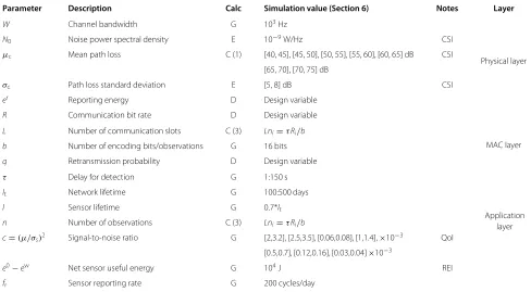
Table 1 lists the essential model parameters and their description. The third column classifies each parameter according to its method of calculation as given from the application knowledge, estimated online, calculated, or as a design parameter. The ‘Notes’ column highlights the parameters that are a measure of the REI, CSI, or QoI for each sensor. The last column classifies each parameter according to its relevant layer in the system model.
4.6 Handshaking overhead
While developing the system model, we ignored the over-head of the handshaking protocol used by the fusion center to collect the quality measures of each sensor, as outlined in Section 3. In this section, we derive the condi-tions that have to be satisfied to ensure that the developed model accuracy is not affected by ignoring the handshak-ing overhead. We measure the protocol overhead by (1) the total delay time taken by the fusion center to collect the quality measures from all sensors in one handshaking cycle (τh) and (2) the total energy spent in the
handshak-ing cycle (eh). We designate the communication rate and
transmission power used by all sensors during the hand-shaking process by Rh andPh, respectively. We further
designate the rate at which the environment changes by
fh(handshaking cycles per day). Our objective is to derive
an upper bound onfhfor a given network that enables us
to ignore the handshaking overhead without affecting the model accuracy. The delay condition could be expressed as
τhfh< α(τfr), (31)
whereαrepresents the allowed percentage of resources to be consumed in the handshaking process, such that the handshaking overhead could be ignored. To calculateτh,
we assume IEEE 754 half-precision binary floating-point format (2 bytes) to represent the quality measures of each
Table 1 Model parameters for the wireless sensor network
Parameter Description Calc Simulation value (Section 6) Notes Layer
W Channel bandwidth G 103Hz
Physical layer
N0 Noise power spectral density E 10−9W/Hz CSI
μc Mean path loss C (1) [40, 45], [45, 50], [50, 55], [55, 60], [60, 65] dB CSI
[65, 70], [70, 75] dB
σc Path loss standard deviation E [5, 8] dB CSI
er Reporting energy D Design variable
R Communication bit rate D Design variable
L Number of communication slots C (3) Lni=τRi/b
MAC layer
b Number of encoding bits/observations G 16 bits
q Retransmission probability D Design variable
τ Delay for detection G 1:150 s
Application layer
lt Network lifetime G 100:500 days
l Sensor lifetime G 0.7*lt
n Number of observations C (3) Lni=τRi/b
c=(μ/σs)2 Signal-to-noise ratio G [2,3.2], [2.5,3.5], [0.06,0.08], [1,1.4],×10−3 QoI [0.5,0.7], [0.12,0.16], [0.03,0.04]×10−3
e0−ew Net sensor useful energy G 104J REI
fr Sensor reporting rate G 200 cycles/day
sensor [32]. According to Table 1, we have five values rep-resenting the sensor quality measures: CSI (N0,μc,σc),
QoI (μ/σs), and REI. Therefore, each sensor requires 10 bytes of payload. Assuming 9 bytes of overhead, the total handshaking delay is given by
τh=
Combining (31) and (32):
fh< α τ fr
152N
Rh. (33)
The energy condition could be expressed as
ehfhl< αe0, (34)
where e0 is the initial energy in each sensor battery, which is assumed the same for all sensors. The energy spent in the handshaking process by each sensor could be expressed as
Combining (34) and (35),
fh< α
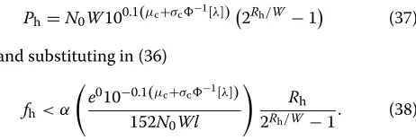
Equations 33 and 36 represent the two conditions that need to be satisfied to ensure that the derived model accu-racy will not be affected by ignoring the handshaking overhead. These two conditions could be verified for any values of the design parametersRhandPh. However, since
we ignored the channel drop probability during the hand-shaking process in the analysis, one more constraint is required to guarantee minimum probability of successful transmission,λ, and hence reliable communication during the handshaking cycle. Since all sensors need to transmit during the handshaking process, we assume that TDMA is the protocol used during handshaking. Accordingly, we can use (2) to get
Ph=N0W100.1(μc+σc
−1[λ])
2Rh/W−1 (37)
and substituting in (36)
fh< α
We note thatfhneeds to satisfy (33) and (38)
simultane-ously. Since the right-hand side of (33) is a monotonically increasing function ofRh and the right-hand side of (38)
is a monotonically decreasing function of Rh, the upper
bound on fh is at the intersection of the two functions.
Hence,
and finally, the upper bound onfhis given by
fh< α τ
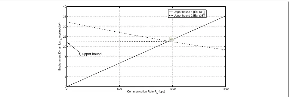
Example 1.We evaluate the upper bound for the exam-ple network simulated in Section 6, where the parameters are shown in Table 1. We useσc = 6dBand an average
value ofμc =50dBfor all sensors. Further, we needλ=
0.9 to ensure reliable communication during the hand-shaking cycle and a percentage of resources consumed in the handshaking α = 0.05. For delay for detectionτ = 25sec, and network lifetimel=250days, we get:
Design parameters : Rh=965bps
Ph=0.56W
Upper bound : fh<22.69cycles/day
Resources consumed : τhfh=242sec/day ehfh=1.94J/day.
(42)
Figure 5 plots the operating point for the two conditions (33) and (38). Accordingly, for the given sensor network, the analysis and the developed model could be used with sufficient accuracy as long as the environment dynam-ics do not require more than 22 cycles/day to update the fusion center. If the environment dynamics are much faster, then the handshaking overhead has to be included in the model development.
5 Transmission control policy design for optimal detection
In Section 4, we developed an integrated model for the detection system, obtained an expression for the detec-tion performance measure (the deflecdetec-tion coefficient), and defined our design constraints. Now, we have the complete optimization problem that we need to solve to obtain the optimal system design variables (sensor communication rateRi, reporting energyeri, and retrans-mission probability for the ALOHA caseqi). We start by summarizing the optimization problem:
0 500 1000 1500 0
5 10 15 20 25 30 35 40
X: 966 Y: 22.7
Communication Rate Rh (bps)
Environment Dynamics f
h
(cycles/day)
Upper bound 1 [Eq. (33)] Upper bound 2 [Eq. (38)]
fh upper bound
Figure 5Handshaking overhead constraints for the example sensor network.
subject to 0≤qi≤1 (ALOHA) (44)
0≤Ri (45)
0≤eri ≤εi i=1, 2,. . .,N (46) N
i=1
eri ≤εt. (47)
In the following discussion, we consider the ALOHA optimization problem only, since the TDMA optimization problem has the same structure, with one of the decision variables omitted (q). We denote the decision variables by
x=q1 . . . qN R1 . . . RN er1 . . . erN
, (48)
wherex ∈ R3N, and the objective function byJ(x). The optimization problem could be rewritten in the form:
min
x −J(x) subject to Ax≥b, (49)
A= ⎡
⎣0 0I −I 0 0 0I 0 0 00
0 0 0 I −I −1
⎤ ⎦
T
, (50)
b= −0 1 0 0 ε εtT. (51)
I is the identity matrix, 0(1) is the vector/matrix of all zeros (ones), with appropriate dimensions, and ε =
ε1 ε2 . . . εN
. We note that our objective function is not convex. Instead of following the classical approach to simplify the system model to obtain a convex func-tion, which may ignore important system dependencies and may lead to a less accurate model, our approach is to analyze the optimization problem to obtain a possible set of candidate points that may speed up the convergence process for existing numerical optimization algorithms, then resort to simulation experiments for performance evaluation.
Although the objective function is not convex, we note that the inequality constraints are linear. Therefore,
the Karush-Kuhn-Tucker (KKT) conditions represent a necessary condition for a local maximizer of the objective function [33]. We first form the Lagrangian:
L(x,ν)= −J(x)−νT(Ax−b), (52)
whereνis the vector of Lagrange multipliers, defined as
νT =ν q0
1 . . . νq0N νq11 . . . νq1N νR1 . . . νRN
νe0
1 . . . νe0N νe1 . . . νeN νeT
(53)
νq0i andνq1i are the Lagrange multipliers for the constraints
in (44),νRiis the Lagrange multiplier for the constraint in
(45),νe0
i andνeiare the Lagrange multipliers for the
con-straints in (46), andνeT is the Lagrange multiplier for the
constraint in (47). We denote the primal and dual optimal points byx∗andν∗, respectively. The KKT conditions are thus given by
−∇J(x∗)−ATν∗=0 (Stationarity) (54)
ν∗T
(Ax∗−b)=0 (Complementary slackness) (55)
(Ax∗−b)0 (Primal feasibility) (56)
ν∗0 (Dual feasibility) (57)
−ZT∇2J(x∗)Z0, (58)
−Z+T∇2J(x∗)Z+0 (59)
where Z+ is a null space matrix for the matrix of non-degenerate active constraints atx∗, i.e., constraints with Lagrange multipliers = 0. The stationarity condition could be expressed as
τ
The given KKT conditions cannot be solved analyti-cally. However, the optimization problem could be solved efficiently using a variety of constrained optimization algorithms, e.g., the interior point method. The following two theorems provide a possible set of candidate points for a local maximizer, hence speeding up the conver-gence process and providing a set of initial points for the optimization algorithm.
Theorem 1. A candidate point for a local maximizer of
the objective function in (43) is when one sensor trans-mits with probability one (q = 1) and maximum energy (eri =εi), while all other sensors remain silent. The optimal
communication rate is given by
R∗i =arg max
Proof. Whenqi = 1, the objective function reduces to
D2=(τ/b)ciRi (ρi)j=i(1−qj). Any value ofqj=0 will
cause the objective function value to decrease. Physically,
qj = 0 corresponds to a guaranteed collision, i.e., loss of information. Therefore, qj = 0. Since Rj anderj do not affect the objective function, we arbitrarily setRj = 0.erj should be set to 0 to save the energy budget for the non-contributing sensor. The solutionqj = Rj = erj = 0 for
j = i could be shown to satisfy the KKT conditions by direct substitution. The objective function monotonically increases witheri. Therefore,eri should be set to its maxi-mum value, i.e.,eri = min(ε,εt). Finally, optimalRi is set to maximize the objective function and, hence, given by (63).
We conclude that we have a set ofNcandidate points, (qi = 1,qj = 0,j = i), for a local maximum, which could be checked easily in N time steps, in addition to the computations required to find the optimal communi-cation rate, which could be implemented efficiently for a single-variable function.
Theorem 2. A candidate point for a local maximizer of
the objective function in (43) is when a subset of the sensors, defined by the index set Sε, transmit with their maxi-mum energy, while all other sensors remain silent. Optimal design variables for the active sensors are at x∗, where
∇J(x∗)=0. The unallocated energy is equal toεt−
i∈Sε
εi.
Proof. For the active sensors, 0 < qi < 1. The total energy constraint is inactive, i.e.,νeT = 0. Iferi < εi, then from the complementary slackness conditionνe0
i =νe1i =
0. From the stationarity condition, we get ∇eriJ = 0, but
∇eriJ = 0 if and only ife
r
i = 0, a contradiction. There-fore, the only option left is eri = εi. In this case, the constraint eri ≤ εi is active; hence, νe0
i = 0. From the
stationarity condition, we get∇er
iJ|eri=εi = νe1
i, which
sat-isfies the dual feasibility condition, since the left-hand side is ≥ 0. Therefore, this point is a candidate for a local maximizer.
We conclude that all active sensors in this case should transmit with maximum energy. Since all other con-straints are inactive, all Lagrange multipliers are equal to 0, and therefore, from the stationarity condition, the opti-mal values forqandRare equal to the stationary pointx∗, where∇J(x∗)=0.
Algorithm 1Optimization Problem Solution
Input:system parameters as in Table 1
Output: optimal decision variables x∗, objective
functionJ(x∗)
setqi = 1/N ∀i,Ri = R0,eri = εt/N {initial pointx0
for the optimization algorithm}
x∗,J(x∗) = OptAlg(J(x),x0, constraints)
We compare our design approach with two other approaches commonly used to design the transmission control policy for practical sensor networks. We do not attempt to compare with specific designs treated in the lit-erature that are optimized for detection applications with very specific hardware configurations not typically used in practical WSNs. We call our approach cross layer design (CLD) hereafter, since it integrates the physical, MAC, and application layers. In both approaches, we assume equal energy allocation scheme, where the energy is divided equally across sensor nodes. This allocation scheme is typically used when sensor quality measures are not inte-grated in the design, and therefore, all sensors are treated equally. Sensor energy is thus given byeri = εt/N. This
allocation scheme is feasible ifεt/N ≤ εi. Otherwise,εi is allocated to each sensor, i.e., eri = min(εt/N,εi). For the special case when all sensors have the same initial and wasted energies, i.e.,e0−ewis the same, we have from (6) and (8)
εt=N(e0−ew)/frlt=(l/lt)Nεi, (64)
whereεiis the same for all sensors. Sincel < lt, we have
εt/N < εi, and therefore, the equal energy allocation is feasible in this case. This case is the one considered in the numerical example in Section 6.4. Finally, we present an upper bound on the system performance to better assess how well the CLD performs compared to the best possible performance, achievable only in theory.
6.1 Maximum throughput design
The throughput for a given WSN is calculated as T =
N
In maximum throughput designs, the design variablesRi andqiare chosen to maximize the throughput in (65). The maximum throughput design thus does not consider the QoI for each sensor. This is clearly shown by comparing (65) to (30), where we note that the maximum throughput design is equivalent to the CLD if all sensors have the same quality of information.
6.2 Decoupled design
In the conventional slotted ALOHA, the MAC sublayer is designed to minimize the probability of collision, without regard to the QoI or CSI of each node. Minimum proba-bility of collision occurs atqi = 1/N. For both ALOHA and TDMA, the physical layer is designed to guarantee a minimum probability of successful packet transmission,λ, i.e.,
Accordingly,Riis given by
Ri=Wlog2
and using (30), the deflection coefficient is given by
D2=
In practice, λ is pre-determined from the application. However, to make a fair comparison, we use the value of λ that maximizes the deflection coefficient in (68), i.e., λ=arg maxλD2, 0≤λ≤1.
6.3 Performance upper bound
6.4 Simulation results
In this section, we evaluate the proposed cross-layer design approach for the system in Figure 1, as com-pared to the classical approaches summarized in Section 6, via a numerical example. We consider a network with 70 sensors (N = 70) deployed for detection, with parameter values as shown in Table 1. To avoid manual entry of parameter values for the 70 sensors, the mean path loss, path loss variance, and the signal-to-noise ratio for each sensor are generated using uniform random number generators. The evaluation is performed both numerically and through Monte Carlo Simulation (MCS) experiments.
6.4.1 Numerical evaluation
We use Algorithm 1 to calculate the optimal solution for the CLD in (30) and the maximum throughput design in (65), where the interior point method is used as the core optimization algorithm. The interior point method is also used to find the optimal probability of successful packet transmission for the decoupled design in (68).
6.4.2 Simulation study
We use the optimal solution for the design variables obtained from the numerical evaluation to set up an MCS for the wireless network, as follows:
• Hypothesis. MCS is performed for bothH0andH1.
to evaluate the deflection coefficient, ROC curve, and probability of error.
• Sensors. Observations are generated locally at each sensor for each communication slot. For ALOHA channels, each sensor attempts transmission
randomly according to its retransmission probability. For TDMA channels, each sensor transmits in its allocated slots only.
• Communication channel. The channel state for each
sensor is simulated for each detection cycle. • Fusion center. The fusion center performs the
likelihood ratio test on the observations received. Equivalently, the fusion center calculates the test statistic in (15) and compares it to a threshold value. • Performance evaluation. The deflection coefficient is
evaluated statistically according to (23). The ROC curve is evaluated by running MCS for different thresholdγ values.
We run the MCS experiment 5,000 times for each delay for detection/network lifetime values to obtain accurate results.
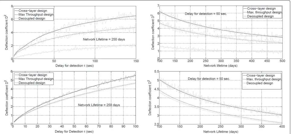
6.4.3 Deflection coefficient
Figure 6, left graph, shows the performance surface for the slotted ALOHA sensor network for the pro-posed CLD approach, for different delay and network
lifetime values. For a fixed network lifetime, the deflection coefficient increases with the delay for detection, as more observations are expected at the fusion center. For a fixed delay for detection, the deflection coefficient decreases with network lifetime. This is mainly because the energy budget allocated for each detection cycle decreases to pro-long the network lifetime. Decreasing the energy budget reduces the probability of successful packet transmission, hence causing less observations at the fusion center. The TDMA sensor network exhibits a similar behavior as illus-trated in Figure 6, right graph. The drop in the deflection coefficient at around 60-s delay and 100-day network lifetime is due to local convergence of the optimiza-tion algorithm. This point represents a local maximum, and a point with larger deflection coefficient could be obtained by varying the initial point of the optimization algorithm.
We resort to two-dimensional plots to compare between the different design approaches. Figure 7, top left graph, shows the deflection coefficient versus the delay for detection for the three design approaches for the ALOHA network, where network lifetime is set to 250 days. The decoupled design approach has the worst performance, even when choosing the optimal value for the probabil-ity of successful transmission λ. This is mainly because the parameters at each layer are specified independently, without regard to the application. The maximum through-put design has a better performance since it seeks to maximize the quantity of the information at the fusion center, by integrating the physical and MAC layers. How-ever, since increasing the quantityof the information is not equivalent to increasing the information quality, as sensors have different QoI, the maximum throughput is outperformed by the proposed CLD approach. The per-formance of the proposed design represents an upper bound on the maximum throughput performance. This upper bound is achieved if all sensors have the same QoI. The MCS results are superimposed on the numerical curves. The simulated results coincide with the numeri-cal results (apart from MCS accuracy), hence verifying the correctness of the analysis.
Figure 6Wireless sensor network performance for the ALOHA (left graph) and TDMA (right graph) sensor networks.
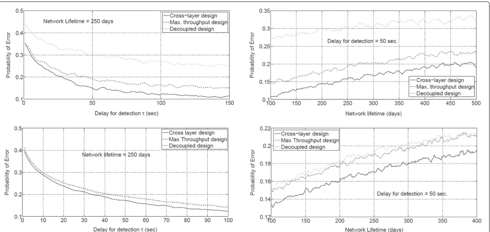
6.4.4 ROC curves
For the probability of error and the ROC curves, we resort to MCS experiments to obtain the performance curves. Figure 8, top left graph, shows the probability of error versus the delay for detection for the ALOHA sensor network, where network lifetime is equal to 250 days. Since the probability of error is directly propor-tional to the deflection coefficient, we obtain the same relative performance, i.e., the proposed CLD approach outperforms the other two approaches, while the max-imum throughput approach outperforms the decoupled design one. The same results are obtained for the proba-bility of error as it varies with the network lifetime, for a fixed delay for detection, which is shown in Figure 8, top right graph. The TDMA sensor network exhibits a similar behavior as illustrated in Figure 8, bottom graphs. The dif-ference between the decoupled design and the maximum throughput design is not noticed in Figure 8, bottom left graph, due to MCS accuracy.
Figure 9 shows the simulated ROC curves for τ =
50 s and lifetime = 250 days and for different values of the thresholdγ ∈[ 0,∞). The figure shows the perfor-mance enhancement using the CLD approach. For the same probability of false alarm, the proposed cross-layer approach results in higher probability of detection than the other approaches. Therefore, by integrating different system layers and quality measures in the design process, we obtain performance enhancement that would not be possible without increasing the delay and/or shortening the network lifetime. Figure 9 also shows the upper bound on the performance, given by (24), whereD2is calculated from MCS assuming no channel drops or contentions. The upper bound is achievable only for ideal channels, and the CLD approaches the upper bound by an amount proportional to the given channel quality.
In practice, a family of these ROC curves are provided for different values of the delay for detection and network lifetimes. The operating point is located on a specific ROC
Figure 8Probability of error for the ALOHA (top graphs) and TDMA (bottom graphs) wireless sensor networks.MCS curves smoothed out for better presentation.
curve, and the relevant values of the detector threshold and the WSN design variables are set accordingly.
7 Slotted ALOHA-TDMA comparison
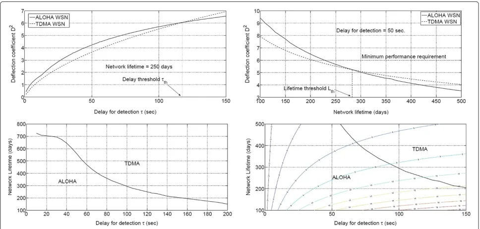
One important question to be answered is whether the TDMA scheme is superior to slotted ALOHA for our detection application. On one hand, elimination of colli-sions results in energy-saving and guaranteed transmis-sion for sensor data. On the other hand, TDMA scheme treats all sensors equally, as it assigns each sensor a time slot while ignoring its quality measures. In this section, we compare the performance of the slotted ALOHA and TDMA sensor networks, based on the numerical example in Section 6. Figure 10, top left graph, shows the deflection coefficient for different delay constraints. We note that the ALOHA network outperforms TDMA if the delay is below
a threshold value, τth. If the delay is increased further,
TDMA outperforms the ALOHA network. For τ < τth,
the ALOHA network outperforms because of its selectiv-ityproperty, where sensors with relatively lower quality measures compared to other sensors are excluded from the detection task. Thisselectivityproperty is lacking in the TDMA network, where all sensors are treated equally and scheduled to transmit their observations, regardless of their quality measures. For τ > τth, TDMA
outper-forms ALOHA, mainly because the average energy per detection cycle (average power) decreases with increasing delay. Therefore, transmission attempts for each sensor for the ALOHA network have to be lowered to con-serve energy wasted in probable collisions. On the other hand, TDMA does not suffer from collisions. Therefore, even with very small energy per detection cycle, sensors
Figure 10ALOHA-TDMA comparison.
may be able to transfer their information to the fusion center, and therefore, the detection performance will be higher. In general, the delay thresholdτth gets higher as
the reporting energy per detection cycle for each sensor,
er, increases. For the given example, the delay thresh-old τth ≈ 120 s. Since detection applications are delay
sensitive, the ALOHA network would be the choice for network design. However, for scarce energy applications, with very low energy per sensor, TDMA maybe a viable alternative.
Figure 10, top right graph, shows the deflection coef-ficient for different lifetime values. Similarly, the TDMA outperforms the ALOHA for lifetime values greater than the threshold lifetime Lth. The threshold lifetime gets
higher as the delay for detection decreases. For the given numerical example, the threshold lifetime Lth ≈ 285
days. Since the performance degrades with increasing net-work lifetime, the deflection coefficient at the threshold lifetime may be below the minimum design value, and therefore, TDMA may not be a feasible design option. For example, in Figure 10, top right graph, the minimum detection performance is specified byD2=6, and there-fore, the ALOHA is the design option. At the threshold lifetime,D2 ≈ 5.2, which is below the minimum design
requirement, and therefore, TDMA cannot be used with such design requirements. However, for scarce energy applications, the threshold lifetime gets smaller, so that TDMA maybe the only viable design option to extend the network lifetime, on the expense of degraded detection performance.
Figure 10, bottom left graph, summarizes the perfor-mance comparison in the delay lifetime two-dimensional
space. The curve represents the boundary between the ALOHA and TDMA regions. For any pair of (delay, life-time) in the ALOHA region, the ALOHA sensor network has a superior performance and similarly for the TDMA region. The figure could be augmented by the contour lines for the deflection coefficient for both ALOHA and TDMA to show the performance measure value. Using the deflection coefficient values, the designer can check whether the selected operating point satisfies the mini-mum performance requirement. Figure 10, bottom right graph, shows the performance regions with the contour lines for the ALOHA region.
8 Conclusion
In this paper, we pursued a cross-layer, model-based approach to design a single-hop ALOHA and TDMA WSNs deployed for detection applications. We developed an integrated model for the detection system that includes the communication network, sensing, and energy models. We considered the QoI, CSI, and REI quality measures in the design process. We designed a complete transmission control policy that includes the transmission probabili-ties, communication rate, and energy allocation for each sensor. We showed a significant performance increase over the decoupled and maximum throughput design approaches with equal energy allocation scheme, for both ALOHA and TDMA networks.
delays, TDMA outperforms the ALOHA network unless the network lifetime is reduced. The designer chooses the best option based on the delay and lifetime constraints, in addition to the minimum allowed performance measure.
The cross-layer design approach results in a no-cost performance increase, since the designer obtains a per-formance increase for the same delay and lifetime con-straints. However, the cross-layer design has its own pitfalls. First, a mathematical model that captures the inter-relationships between different layers has to be developed. This model is, in general, complex, and it maybe required to go through the design process sev-eral times to refine the assumptions in order to obtain a tractable model. Second, the optimization problem obtained has to be solvable in real time with existing optimization algorithms. This is not always possible, as the optimization problem complexity is closely coupled to the model complexity. Finally, the optimality of the design depends on the availability of the global informa-tion in real time. This assumpinforma-tion may not always be true in practice. Despite these pitfalls, the cross-layer design complexity is justified when it is desired to optimize the performance with limited system resources that cannot be replenished (e.g., remote WSN in a battlefield). The decoupled approach, on the other hand, maybe justified for systems with enough resources such that the perfor-mance loss could be compensated by additional resource allocation.
Several extensions could be made to the work pre-sented in this paper. Multi-hop sensor networks could be addressed instead of single-hop networks. Small-scale fading could be incorporated in the system model, provid-ing a more general model that is applicable in a variety of sensor network applications. Finally, other channel access schemes could be considered, e.g., FDMA, CDMA, and SDMA.
Competing interests
The authors declare that they have no competing interests.
Acknowledgements
This work is supported in part by the National Science Foundation (CNS-1238959, CNS-1035655).
Author details
1Global Operations Organization, British Petroleum Egypt, Cairo 11728, Egypt. 2Institute for Software Integrated Systems, Department of Electrical Engineering and Computer Science, Vanderbilt University, Nashville, TN 37235, USA.
Received: 8 October 2013 Accepted: 10 March 2014 Published: 31 March 2014
References
1. R Viswanathan, P Varshney, Distributed detection with multiple sensors I. Fundamentals. Proc. IEEE.85, 54–63 (1997)
2. AS Abu-romeh, DL Jones, Decentralized detection in censoring sensor networks under correlated observations. EURASIP J. Adv. Signal Process. 2010, 1–10 (2010)
3. T Duman, M Salehi, Decentralized detection over multiple-access channels. IEEE Trans. Aerosp. Electron. Syst.34(2), 469–476 (1998) 4. M Longo, T Lookabaugh, R Gray, Quantization for decentralized
hypothesis testing under communication constraints. IEEE Trans. Inform. Theory.36(2), 241–255 (1990)
5. VV Veeravalli, JF Chamberland, ed. by A Swami, Q Zhao, TW Hong, and Tong L, Detection in sensor networks, inWireless Sensor Networks: Signal Processing and Communications Perspectives(Wiley West Sussex, 2007), pp. 119–148
6. L Liu, JF Chamberland, Cross-layer optimization and information assurance in decentralized detection over wireless sensor networks (2006). Paper presented at the fortieth Asilomar conference on signals, systems and computers (ACSSC ’06), Asilomar, CA, USA, 29 Oct–1 Nov 2006, 271–275 (2006)
7. IEEE Computer Society,IEEE Standard for Local and Metropolitan Area Networks–Part 15.4: Low-Rate Wireless Personal Area Networks (LR-WPANs). (IEEE, New York, 2011)
8. JN Tsitsiklis, ed. by HV Poor, JB Thomas, Decentralized detection, in Advances in Signal Processing(JAI Press Oxford, 1993), pp. 297–344 9. M Gastpar, Uncoded transmission is exactly optimal for a simple Gaussian
sensor network. IEEE Trans.Inform. Theory.54(11), 5247–5251 (2008) 10. A Tantawy, X Koutsoukos, G Biswas, Transmission control policy design
for decentralized detection in tree topology sensor networks. Paper presented at the 14th international conference on information fusion, Chicago, IL, USA, July 5–8 2011, 1–8
11. A Tantawy, X Koutsoukos, G Biswas, A cross-layer design for decentralized detection in tree sensor networks. Paper presented at the IEEE international conference on distributed computing in sensor systems (DCOSS), Hangzhou, China, 16–18 May 2012
12. B Chen, R Jiang, T Kasetkasem, PK Varshney, Channel aware decision fusion in wireless sensor networks. IEEE Trans. Signal Process. 52(12), 3454–3458 (2004)
13. Y Yilmaz, GV Moustakides, X Wang, Channel-aware decentralized detection via level-triggered sampling. IEEE Trans. Signal Process. 61, 300–315 (2013)
14. G Mergen, V Naware, L Tong, Asymptotic detection performance of type-based multiple access over multiaccess fading channels. IEEE Trans. Signal Process.55(3), 1081–1092 (2007)
15. YW Hong, PK Varshney, ed. by A Swami, Q Zhao, YW Hong, and L Tong, Data-centric and cooperative MAC protocols for sensor networks, in Wireless Sensor Networks: Signal Processing and Communications (Wiley West Sussex, 2007), pp. 311–344
16. Y Yuan, M Kam, Distributed decision fusion with a random-access channel for sensor network applications. IEEE Trans. Instrum. Meas. 53(4), 1339–1344 (2004)
17. TY Chang, TC Hsu, PW Hong, Exploiting data-dependent transmission control and MAC timing information for distributed detection in sensor networks. IEEE Trans. Signal Process.58(3), 1369–1382 (2010) 18. YW Hong, KU Lei, CY Chi, Channel-aware random access control for
distributed estimation in sensor networks. IEEE Trans. Signal Process. 56(7), 2967–2980 (2008)
19. Y Yang, R Blum, B Sadler, Energy-efficient routing for signal detection in wireless sensor networks. IEEE Trans. Signal Process.57(6), 2050–2063 (2009)
20. Y Sung, S Misra, L Tong, A Ephremides, Cooperative routing for distributed detection in large sensor networks. IEEEJ. Select. Areas Commun.25(2), 471–483 (2007)
21. Q Zhao, A Swami, L Tong, The interplay between signal processing and networking in sensor networks. IEEE Signal Process. Mag.23(4), 84–93 (2006)
22. A Tantawy, X Koutsoukos, G Biswas,Transmission control policy design for decentralized detection in sensor networks
23. R Gallager,Principles of Digital Communication. (Cambridge University Press, New York, 2008)
24. S Salous,Radio Propagation Measurement and Channel Modelling, 1st edn. (Wiley, West Sussex, 2013)
25. F Zhao, L Guibas,Wireless Sensor Networks: An Information Processing Approach. (Morgan Kaufmann, New York, 2004)
27. M Bhardwaj, T Garnett, A Chandrakasan, Upper bounds on the lifetime of sensor networks. ICC.3, 785–790 (2001)
28. J Deng, Y Han, W Heinzelman, P Varshney, Scheduling sleeping nodes in high density cluster-based sensor networks. Mobile Netw. Appl. 10(6), 825–835 (2005)
29. Y Chen, Q Zhao, On the lifetime of wireless sensor networks. IEEE Commun. Lett.9(11), 976–978 (2005)
30. SM Kay,Fundamentals of Statistical Signal Processing: Detection Theory, vol. 2. (Prentice Hall, New Jersey, 1998)
31. B Picinbono, On deflection as a performance criterion in detection. IEEE Trans. Aerosp. Electron. Syst.31(3), 1072–1081 (1995)
32. IEEE,IEEE Standard 754-2008: IEEE Standard for Floating-Point Arithmetic. (IEEE, New York, 2008)
33. S Boyd, L Vandenberghe,Convex Optimization. (Cambridge University Press, Cambridge, 2004)
doi:10.1186/1687-6180-2014-43
Cite this article as:Tantawyet al.:Cross-layer design for decentralized
detection in WSNs. EURASIP Journal on Advances in Signal Processing
20142014:43.
Submit your manuscript to a
journal and benefi t from:
7Convenient online submission
7Rigorous peer review
7Immediate publication on acceptance
7Open access: articles freely available online
7High visibility within the fi eld
7Retaining the copyright to your article