FULL PAPER
3D inversion of full gravity gradient
tensor data in spherical coordinate system using
local north-oriented frame
Yi Zhang
1, Yulong Wu
1*, Jianguo Yan
2, Haoran Wang
3,4, J. Alexis P. Rodriguez
5and Yue Qiu
6Abstract
In this paper, we propose an inverse method for full gravity gradient tensor data in the spherical coordinate system. As opposed to the traditional gravity inversion in the Cartesian coordinate system, our proposed method takes the curvature of the Earth, the Moon, or other planets into account, using tesseroid bodies to produce gravity gradient effects in forward modeling. We used both synthetic and observed datasets to test the stability and validity of the proposed method. Our results using synthetic gravity data show that our new method predicts the depth of the den-sity anomalous body efficiently and accurately. Using observed gravity data for the Mare Smythii area on the moon, the density distribution of the crust in this area reveals its geological structure. These results validate the proposed method and potential application for large area data inversion of planetary geological structures.
Keywords: Gravity gradient tensor, Inversion, Density distribution, Spherical coordinate system, Local north-oriented frame
© The Author(s) 2018. This article is distributed under the terms of the Creative Commons Attribution 4.0 International License (http://creativecommons.org/licenses/by/4.0/), which permits unrestricted use, distribution, and reproduction in any medium, provided you give appropriate credit to the original author(s) and the source, provide a link to the Creative Commons license, and indicate if changes were made.
Introduction
The gravity gradient tensor (GGT) is the second deriva-tive of the gravity potential. Compared to the general gravity field Tz, GGT contains nine components and has
much higher resolution in inverting the spatial position of target anomaly bodies, which means it will offer more information to better understand the interior structure of the earth or some other planets (Li 2001; Bouman et al.
2016).
In 1886, a torsion balance gradiometer was first devel-oped by Lorand Eotvos, becoming a useful tool for mining and hydrocarbon exploration (Pedersen and Ras-mussen 1990; Bell and Hansen 1998). 3D inversion of GGT data was originally introduced by Vasco (1989) and Vasco and Taylor (1991), who focused on the covariance and resolution measures of the solution appraisal. More recently, several algorithms were developed to inverse GGT data (e.g., Li 2001; Zhdanov et al. 2004; Uieda and
Barbosa 2012; Oliveira and Barbosa 2013; Martinez et al. 2012; Geng et al. 2015; Meng 2016). The differ-ences among these algorithms are related to the choice of model object functions in the inversion procedure; all the model object functions can be retraced back to the inver-sion methods used in the inverinver-sion of the general gravity field (e.g., Last and Kubik 1983; Guillen and Menichetti
1984; Barbosa and Silva 1994; Li and Oldenburg 1996,
1998; Farquharson 2008).
In addition to the choice of model object functions, there is little agreement on best component of GGT for the inversion. Li (2001) combined five independent com-ponents excluding Tzz. Zhdanov et al. (2004) used the
horizontal components Txy and Tuv= (Txx−Tyy)/2.
Mar-tinez et al. (2012) combined the horizontal components and Tzz. Capriotti et al. (2015) employed a combination
of the GGT and general gravity field Tz. Pilkington (2012)
used an eigenvalue spectra method to evaluate the utility of combining different GGT components, preferring the
Tzz component, indicating that the source-model
infor-mation is improved by adding more components only at close distance to the anomaly sources. Later, Pilkington (2013) used estimated parameter errors from parametric
Open Access
*Correspondence: [email protected]
1 Key Laboratory of Earthquake Geodesy, Institute of Seismology, China Earthquake Administration, 48 Hongshan Side Road, Wuhan 430071, Hubei, China
Page 2 of 23 Zhang et al. Earth, Planets and Space (2018) 70:58
inversions, concluding that the Tzz component gave the
best performance, while the horizontal components Txx
and Tyy performed poorly. Paoletti et al. (2016) used
a singular value decomposition (SVD) tool to analyze both synthetic data and gradiometer measurements. This research showed that the main factors controlling the reliability of the inversion are algebraic ambiguity (the difference between the number of unknowns and the number of available data points) and signal-to-noise ratio.
All these inversion methods mentioned are imple-mented in the Cartesian coordinate system (CCS). For small-scale problems such as mining or hydrocarbon exploration on earth, the target area is usually relatively small compared to the radius of the earth and can be considered as a flat surface, so inversion in CCS works fine and obtains reliable inversion results with high accu-racy. However, for large-scale inversion problems, such as density imaging of the lunar mascon with the satel-lite gravity datasets, the target area of the lunar mascon was usually large and covered an area with hundreds or thousands of kilometers in both longitude and latitude directions. Moreover, the radius of the moon was rela-tively small (1738 km), and this meant the inversion area of the mascon was no longer a flat area; hence, inversion methods cannot ignore the influences of the lunar curva-ture. To deal with this problem, the inversion method in the SCS must be considered. Liang et al. (2014) extended Li and Oldenburg’s (1996, 1998) inversion method to the SCS using the general gravity field.
In the history of the Moon exploration, one of the most amazing discoveries was the concentrated areas of mass found on the near side of the moon (Muller and Sjogren
1968; Melosh et al. 2013; Freed et al. 2014). These con-centrated areas of mass, referred to as mascons, usually have a positive gravity anomaly peak and surrounded by negative gravity anomalies with low geographical eleva-tion. The knowledge of the interior density structure of mascons will help to understand its origin mechanism (Wang et al. 2015; Jansen et al. 2017). There has a signifi-cant improvement on lunar gravity field model develop-ment (Matsumoto et al. 2010; Yan et al. 2012), and the recent high solution gravity field model GL1500E derived from GRAIL mission (The Planetary Data System 2016) makes it possible to investigate the interior density struc-ture of the mascons (Zuber et al. 2013a, b) using lunar gradient data.
The high-resolution lunar gradient data produced from GRAIL gravity was applied by Andrews-Hanna et al. (2014) to investigate the structure and evolution of the lunar Procellarum region. The fault geometry, thermal structure, and material content were considered to gener-ate rectilinear patterns of the gradient data in this region.
A forward modeling method coupling with finite element method (FEM) was employed this work. GGT is the dif-ference of gravity in different directions, which helps to remove the influence of the long-wave part in the lunar gravity, and it is easier to highlight the lunar gravity’s shortwave effect and to get a better resolution for density imaging. In this work, we will focus on inversion of the lunar gradient data, which is different from the previous work (Andrews-Hanna et al. 2013).
The remainder of this paper is as follows: a brief intro-duction of this inversion method is presented in second section. Third section details two different models and experiments with synthetic GGT datasets and inversion of GGT observation datasets of moon. The interior den-sity structure of the Mare Smythii mascon is discussed in fourth section. Finally, in fifth section we present the conclusions of this study.
Methodology
GGT in the spherical coordinate system
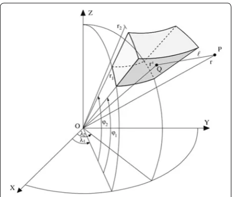
The two most commonly used frames in SCS are the geocentric spherical frame (GSF) and the local north-oriented frame (LNOF). The GGT is expressed in terms of the second derivatives of the gravitational potential U
in the r, λ, and ϕ directions of GSF, where r, λ, and ϕ refer to the radial, longitude, and latitude, respectively (Eq. 1).
In LNOF, where z has the geocentric radial downward direction, x points to the north, and y is directed to the east with a right-handed system, relationship between the LNOF and GSF can be described as in Eq. (2) (Reed
1973; Petrovskaya and Vershkov 2006).
In this paper, we choose to use LNOF, which will not be singular when calculating GGT components from a gravity spherical harmonics model (Eshagh 2008, 2010) and because the GGT is symmetric and the trace of the
GGT equals zero; hence, there are only five independent components.
Forward modeling
Theoretically, forward modeling is the basis of the inver-sion, as it forms the relationship between the model and data space. The forward modeling method we use here was developed by Asgharzadeh et al. (2007) for calculat-ing a gravity field and its gradients in the SCS with LNOF. This method makes use of the Gauss–Legendre quad-rature integration for numerically modeling theoretical gravity effects caused by the tesseroids (Anderson 1976; Heck and Seitz 2006) (Fig. 1).
According to Asgharzadeh et al. (2007), each compo-nent of the GGT can form its own relationship between the model and dataset and can be described as:
In Eq. (3), m and Gij refer to the model and kernel
matrix, respectively.
To make full use of the GGT dataset, we adopt the new kernel function G as the linear combination of the five independent components of GGT:
kij here refers to the weighting factor of each
compo-nent, and it can be considered as the data accuracies (or the reliabilities) of each component.
Due to the relationship of Txx+Tyy+Tzz= 0, the
lin-ear combination of the components Txx and Tyy can be
described by the vertical components Tzz; hence, we do
not employ the components Txx and Tyy in Eq. (4).
Similarly, the GGT dataset ds can be also adopted into
the linear combination of the independent components:
For each independent component Tij, the error
stand-ard deviation is σij. According to error theory, the error
standard deviation of the GGT will be:
In Eq. (6), Cov represents the sum of the error covari-ance of all components. On the assumption that the error of the GGT follows the Gaussian random distribution and one independent component has no connection with each other, then Cov= 0.
In general, because of an insufficient observed dataset, the multiple solutions problem becomes a serious issue for the 3D gravity inversion. To deal with the problem, a suitable model objective function is required.
Li and Oldenburg (1996) and Li (2001) designed a model objective function with a maximum smoothing method; however, this model objective function is only suitable for CCS. Liang et al. (2014) extended it to the SCS using the spherical derivative operators:
The model object function of Eq. (7), also called sta-bilized function, was initially introduced by Backus and Gilbert (1967, 1968, 1970) to solve ill-posed inverse problems. It can be divided into two parts: the first item of Eq. (7) is the smallest model between recovered and reference model, and the last three items are the smooth-est model between recovered and reference model in
(7)
Page 4 of 23 Zhang et al. Earth, Planets and Space (2018) 70:58
longitudinal, latitudinal, and radial directions, respec-tively. In Eq. (7), m and mref refer to the recovered and
reference model, respectively. αi (i=s, r, λ, ϕ) are length
scales, which control the balance of the smoothness ver-sus smallness for the whole model, αs for smallness, and
αr, αλ, and aϕ for smoothness (Oldenburg and Li 2005;
Williams 2008). In practice, αs usually can be assigned to
a value of 1.0 or other suitable value; however, different to those in CCS (Williams 2008), αλ, and aϕ are variable
because of the different tesseroid body sizes along the radial direction. w(r) here represents the depth weight-ing function, and it can be used to avoid the skin effect in the inversion (Li and Oldenburg 1996; Li 2001). The depth weighting functions match the decay of the gravity or magnetic kernel functions, and they are in proportion to 1/r2 in gravity and 1/r3 in magnetic inversion problem.
Without them, the inversion will get results concentrated on the surface of the target area (Li 2001). Unlike the uniform prism cells in CCS, the tesseroid cells become smaller along the radial direction from surface to the core, so it must rescale them into the same level. Liang’s et al. (2014) main contribution is the modification of the depth weighting function in SCS by rescaling the cell vol-ume to the surface (see Additional file 1).
In Eq. (8), R is the radius of the reference sphere and H
is the average height of observed dataset above the refer-ence sphere, while r0 and r are the radial distance of the
surface and for computing tesseroid cells, respectively. In addition, geological and geophysical constraints play an important role in the gravity inversion. The geologi-cal and geophysigeologi-cal constraints are varied, and they can be classified into two different kinds: (1) geometry con-straints like structure boundaries, orientations, and loca-tions information; (2) physical property constraints such as surface material content and information from drill holes. All these constraints can be described as the func-tion of the physical property and posifunc-tions. In our inver-sion method, as we divided the subspace into different tesseroid cells, the constraints become the function of
(8) w2(r)= r
2
r2
0(H+R−r)2
the physical property and index number of the tesseroid cells.
Different from the model objective function, which aims to solve the non-uniqueness in ill-posed inverse problems, the purpose of using a prior geological and geophysical information during the inversion is to improve the inversion result. In this paper, we use the Lagrangian multipliers method, introduced by Zhang et al. (2015), to fit for the different prior geological or geophysical information during the inversion procedure; the additional penalty function of the density bound con-straints makes the recovered model more reliable.
Examples of synthetic GGT data
In this section, we will give two examples of the artificial synthetic model used to validate our inversion method.
Single model
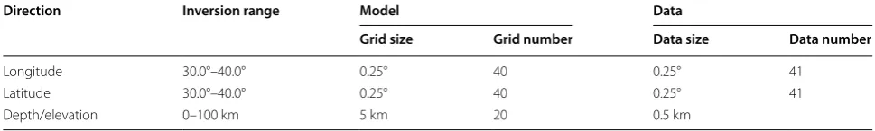
Table 1 shows the 3D mesh and dataset setting for inver-sion. The reference radius we use is 1738 km, which is the same as the mean radius of the moon.
The artificial synthetic model we use here is a horizon-tal spherical prism body with constant residual density of 0.5 g/cm3 and covers an area of 33°–37° in both the
lon-gitude and latitude directions as well as 1648–1698 km in radial direction. The background density was set to 0 g/ cm3. Figure 2 shows the horizontal slice and vertical
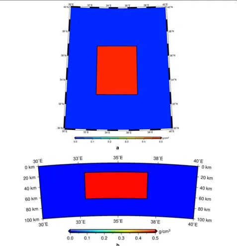
pro-file of the artificial synthetic model used for inversion. In Figs. 3, 4, we showed the artificial theoretical data-sets for all the components of the GGT. Considering the geometric relationships between the model mesh and the data grids in Table 1, we also obtained the kernel matrixes Gs=Gxy+Gxz+Gyz+Gzz and the GGT dataset
ds=dxy+dxz+dyz+dzz, as shown in Fig. 4c.
Furthermore, independent Gaussian random noise was added to each component of the GGT dataset. The mean value of the Gaussian noise was zero, the standard devia-tion was approximately 1% of the difference between the maximum and minimum value of each component, and the artificial theoretical datasets with noise are shown in Figs. 5, 6.
In the inversion, we assigned a density constraint between 0 and 0.5 g/cm3 to each inverted cell. The
L-curve method (Calvetti et al. 2000) was used to search
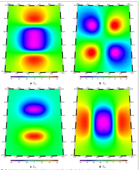
Table 1 3D mesh and dataset for inversion
Direction Inversion range Model Data
Grid size Grid number Data size Data number
Longitude 30.0°–40.0° 0.25° 40 0.25° 41
Latitude 30.0°–40.0° 0.25° 40 0.25° 41
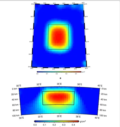
for the best Tikhonov regularization parameter (Tik-honov and Arsenin 1977), and the recovered model is shown in Fig. 7. Tikhonov regularization parameter here is the trade-off between the model objective function and data objective function (also named data misfit). The Tik-honov regularization parameter we chose is 10, which is located at the corner of L-curve, but slightly offset to the right with a smaller data misfit (Zhang et al. 2015). The
black lines in Fig. 7 indicate the boundary of the artificial synthetic model, and the recovered model was fitted well. The recovered model with minimum-structure inversions using L2-norm measures usually has blurred boundaries,
and if sharp boundaries and blocky features are needed, the non-L2 inversions may provide an alternative method
(Sun and Li 2014).
Page 6 of 23 Zhang et al. Earth, Planets and Space (2018) 70:58
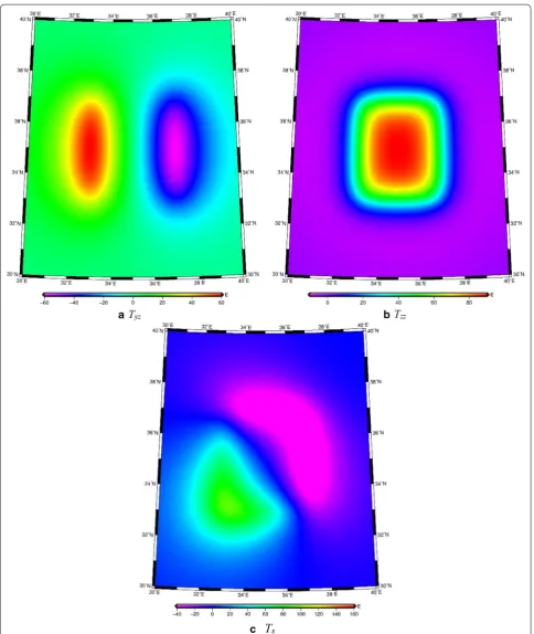
Fig. 4 Artificial theoretical datasets of the GGT for single model, a and b are Tyz and Tzz components of the GGT, respectively, and c Ts is the
Page 8 of 23 Zhang et al. Earth, Planets and Space (2018) 70:58
Fig. 6 Artificial theoretical datasets of the GGT with noise for single model, a and b are Tyz and Tzz components of the GGT, respectively, and c Ts is
Page 10 of 23 Zhang et al. Earth, Planets and Space (2018) 70:58
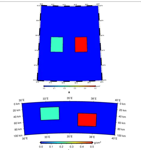
Composite models
Here we designed two composite models. One model covered an area of 34°–36°, 32°–34°, and 1678–1718 km in latitude and longitude as well as radial direction, respectively, with a small residual density of 0.2 g/cm3.
The residual density of the other model was 0.7 g/cm3,
and its geological setting was 34°–36°, 36°–38°, and 1658–1698 km in latitude and longitude as well as radial direction, respectively. The 3D mesh and dataset set-tings we used are shown in Table 1. The horizontal slice and vertical profile of the artificial synthetic models are shown in Fig. 8.
Similarly, we obtained the artificial theoretical datasets of all the components of the GGT (Figs. 9, 10), as well as the added 1% Gaussian random noise, as shown in Figs. 11, 12.
Using the same scheme, with a density bound of 0–0.7 g/cm3, the recovered model was obtained, as in
Fig. 13; the recovered model was well fitted with the blank lines indicating the boundaries of the theoretical models.
Through the artificial theoretical models, we tested our inversion method in the SCS with LNOF. The results indicated that the method is possible to be employed in interior density structure model inversion. In the next
Page 12 of 23 Zhang et al. Earth, Planets and Space (2018) 70:58
Fig. 10 Artificial theoretical datasets of the GGT for composite models, a and b are Tyz and Tzz components of the GGT, respectively, and c Ts is the
Page 14 of 23 Zhang et al. Earth, Planets and Space (2018) 70:58
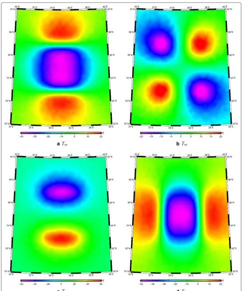
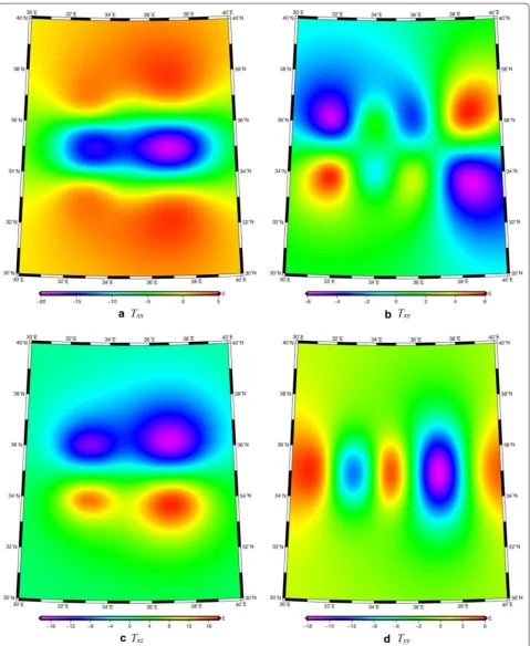
Fig. 11 Artificial theoretical datasets of the GGT with noise for composite models, a, b, c and d are Txx, Txy, Txz and Tyy component of the GGT,
Page 16 of 23 Zhang et al. Earth, Planets and Space (2018) 70:58
Fig. 13 Recovered density distribution for composite models. a Horizontal slice of the recovered model with a radial length of 1698 km, b vertical profile of the recovered model at the latitude of 35°
Table 2 3D mesh and datasets for the inversion of Mare Smythii
Direction Inversion range Model Data
Grid size Grid number Data size Data number
Longitude 76.0°–97.0° 0.25° 84 0.25° 85
Latitude − 10.0°–9.0° 0.25° 76 0.25° 77
section, we will make use of the actual lunar GGT data-sets to validate our inversion method.
Inversion of GGT data at lunar mascon
We selected the Mare Smythii mascon as an exam-ple. The Mare Smythii is a lunar mare located along the equator on the easternmost edge of the lunar near side (Wilhelms 1987). According to Liang et al. (2014), our model mesh should have a grid size that approximately equaled to 8 km, i.e., 0.25° by 0.25° on sphere (Table 2),
which meant the suitable maximum degree of the lunar gravity model should be 720. Hence, the GGT datasets of this mare derived from lunar gravity field GL1500E with a degree and order up to 720 (The Planetary Data System
2016) are shown in Figs. 14, 15, and the expressions for GGT in LNOF we used came from spherical harmonics (Eshagh 2010). We used a Bouguer correction to remove the gravity effect of the lunar topography and deployed a Gaussian averaging function with an averaging radius of 10 km, which matched the size of the divided cells, to
Page 18 of 23 Zhang et al. Earth, Planets and Space (2018) 70:58
reduce the leakage errors caused by high-degree spheri-cal harmonic coefficients. Actually, the Gaussian averag-ing function was proved to be double-edged (Jekeli 1981); if the selected radius was too large, the filter will remove the useful information and the calculated components will be too smooth. In this paper, we preferred to choose
a smaller Gaussian averaging radius which keeps more useful details.
The spherical harmonic coefficients below degree 6 were removed from the GGT datasets we used, and the gravity signal from the left degrees was assumed to be only affected by the lunar crust. The average density of
Fig. 15 Lunar GGT datasets derived from GL1500E, a and b are Tyz and Tzz components of the lunar GGT, respectively, and c Ts is the summation of
the lunar crust we use here is generally 2.56 g/cm3, at a
range of 2.30–2.90 g/cm3 (Wieczorek et al. 2013). This
was also considered as the geological constraint during the inverse process. The 3D mesh and datasets for the inversion of the Mare Smythii are described in Table 2.
By using the GGT datasets as well as the density bounds, we produced an image of the relative density dis-tribution of the Mare Smythii, as shown in Figs. 16, 17
and 18, and the density distribution shows that the depth of Mare Smythii is deeper than which referred from Wieczorek et al. (2013) and similar with the result from Andrews-Hanna et al. (2013).
The gravity gradient reflects the density anomaly; Figs. 16, 17 and 18 shows that there are multi-ring struc-tures (Spudis 1993) at the Mare Smythii site. As the density distribution of the Mare Smythii we extracted
Page 20 of 23 Zhang et al. Earth, Planets and Space (2018) 70:58
through inversion showed some annulus density struc-tures in the shallow stratums and these annulus density structures had the mascon center as the origin point, therefore we infer that there are significant density changes occurred from inside to outside. The formation of these annulus density structures is possibly explained by impacts and crater excavations (Melosh et al. 2013; Montesi 2013). When impacts occur, the kinetic energy is intense and is transformed into heat; this may cause
melting and even vaporize the lunar crust, with cracked lunar crust rocks splashing out of the impact basin. After an impact, a rebalancing of the lunar crust and mantle will likely promote an uplifting of the deeper magma to fill in or eject around an impact basin. The density dif-ference as well as the distance of an ejection could be the reason behind the annulus density structures in this area.
The recovered Ts (Fig. 19a) is similar to the original Ts
shown in Fig. 15c and the data residual in Fig. 19b, and
the difference between original Ts and recovered Ts also
meets our standard deviation expectation of about 5 E. From Fig. 19b, we can see that the residuals inside the Mare Smythii region are close to zero, and it means the good performance of our inversion method. The random big residual values at the verge are caused by the bound-ary effects.
Conclusion
An inversion method is fundamental when developing an advanced understanding of the interior structure of planetary geological structures. We presented an effec-tive algorithm that uses full gravity gradient tensor data in spherical coordinate system using local north-oriented frame. In the test case using simulated data, we used two
Fig. 18 Relative density distribution for different depths at Mare Smythii area, a and b are 80 ~ 85 km, 90 ~ 95 km, respectively
Page 22 of 23 Zhang et al. Earth, Planets and Space (2018) 70:58
different models, single and composite models. By check-ing the differences between the simulated and recovered models, we demonstrated the reliability of our method. We also tested the method on observed data from the Mare Smythii mascon area located on the lunar near side and obtained its interior density distribution. This method could also be applied more generally in magnetic data inversion and in exploratory studies of geological structures of large areas.
Abbreviations
GGT: gravity gradient tensor; SCS: spherical coordinate system; CCS: Cartesian coordinate system; SVD: singular value decomposition; FEM: finite element method; GSF: geocentric spherical frame; LNOF: local north-oriented frame.
Authors’ contributions
YZ and JY conceived and designed the experiment; YZ performed the computation; YW analyzed the data; HW interpreted the results; and JAPR and YQ discussed the results and polished the manuscript. YZ and JY wrote the paper, and all the authors improved it. All authors read and approved the final manuscript.
Author details
1 Key Laboratory of Earthquake Geodesy, Institute of Seismology, China Earthquake Administration, 48 Hongshan Side Road, Wuhan 430071, Hubei, China. 2 State Key Laboratory of Engineering in Surveying, Mapping and Remote Sensing, Wuhan University, 129 Luoyu Road, Wuhan 430070, Hubei, China. 3 MOE Key Laboratory of Fundamental Physical Quantities Measurement, School of Physics, Huazhong University of Science and Technol-ogy, 1037 Luoyu Road, Wuhan 430074, Hubei, China. 4 Hubei Key Laboratory of Gravitation and Quantum Physics, School of Physics, Huazhong University of Science and Technology, 1037 Luoyu Road, Wuhan 430074, Hubei, China. 5 Planetary Science Institute, 1700 East Fort Lowell Road, Suite 106, Tucson, AZ 85719-2395, USA. 6 DFH Satellite Co. LTD, 104 Youyi Road, Beijing 100094, China.
Acknowledgements
The authors thank Stephen McClure for fruitful and informative discussions.
Competing interests
The authors declare that they have no competing interests.
Data and resources
The source codes for this work can be obtained by contacting the corre-sponding author. Some of the figures were produced using Generic Mapping Tools (GMT).
Funding
This work is supported by grant of the National Natural Science Foundation of China (41374024, 41704082), Director Foundation of the Institute of Seis-mology, China Earthquake Administration (IS201616249), Key Laboratory of Geospace Environment and Geodesy, Ministry of Education, Wuhan University (16-01-02), and Hubei Province Natural Science Foundation innovation group Project (2015CFA011).
Publisher’s Note
Springer Nature remains neutral with regard to jurisdictional claims in pub-lished maps and institutional affiliations.
Received: 15 September 2017 Accepted: 27 March 2018 Additional file
Additional file 1. Length scale in spherical coordinate system.
References
Anderson EG (1976) The effect of topography on solutions of Stokes’ problem, Unisurv S-14, Rep, School of Surveying, University of New South Wales, Kensington
Andrews-Hanna JC, Asmar SW, Head JW, Kiefer WS, Konopliv AS, Lemoine FG, Matsuyama I, Mazarico E, McGovern PJ, Melosh HJ, Neumann GA, Nimmo F, Phillips RJ, Smith DE, Solomon SC, Taylor GJ, Wieczorek MA, Williams JG, Zuber MT (2013) Ancient igneous intrusions and early expansion of the Moon revealed by GRAIL gravity gradiometry. Science 339:675–678. https://doi.org/10.1126/science.1231753
Andrews-Hanna JC, Besserer J, Head JW III, Howett CJA, Kiefer WS, Lucey PJ, McGovern PJ, Melosh HJ, Neumann GA, Phillips RJ, Schenk PM, Smith DE, Solomon SC, Zuber MT (2014) Structure and evolution of the lunar Procellarum region as revealed by GRAIL gravity data. Nature 514:68–71. https://doi.org/10.1038/nature13697
Asgharzadeh MF, von Frese RRB, Kim HR, Leftwich TE, Kim JW (2007) Spherical prism gravity effects by Gauss–Legendre quadrature integration. Geo-phys J Int 169:1–11. https://doi.org/10.1111/j.1365-246X.2007.03214.x Backus G, Gilbert J (1967) Numerical applications of a formalism for
geophysi-cal inverse problems. Geophys J R Astron Soc 13:247–276. https://doi. org/10.1111/j.1365-246X.1967.tb02159.x
Backus G, Gilbert F (1968) The resolving power of gross Earth data. Geophys J R Astron Soc 16:169–205. https://doi.org/10.1111/j.1365-246X.1968. tb00216.x
Backus G, Gilbert F (1970) Uniqueness in the inversion of inaccurate gross Earth data. Philos Trans R Soc Lond Ser A Math Phys Sci 266:123–192 Barbosa V, Silva J (1994) Generalized compact gravity inversion. Geophysics
59:57–68. https://doi.org/10.1190/1.1443534
Bell R, Hansen R (1998) The rise and fall of early oil field technology: the torsion balance gradiometer. Lead Edge 17:81–83. https://doi. org/10.1190/1.1437836
Bouman J, Ebbing J, Fuchs M, Sebera J, Lieb V, Szwillus W, Haagmans R, Novak P (2016) Satellite gravity gradient grids for geophysics. Sci Rep 6:21050. https://doi.org/10.1038/srep21050
Calvetti D, Morigi S, Reichel L, Sgallari F (2000) Tikhonov regularization and the L-curve for large discrete ill-posed problems. J Comput Appl Math 123:423–446. https://doi.org/10.1016/S0377-0427(00)00414-3 Capriotti J, Li Y, Krahenbuhl R (2015) Joint inversion of gravity and gravity
gradient data using a binary formulation. In: International workshop and gravity, electrical & magnetic methods and their applications, Chenghu, China, 19–22 April 2015. Society of Exploration Geophysicists and Chinese Geophysical Society, pp 326–329. https://doi.org/10.1190/ gem2015-085
Eshagh M (2008) Non-singular expressions for the vector and the gradient tensor of gravitation in a geocentric spherical frame. Comput Geosci 34:1762–1768. https://doi.org/10.1016/j.cageo.2008.02.022 Eshagh M (2010) Alternative expressions for gravity gradients in local
north-oriented frame and tensor spherical harmonics. Acta Geophys 58:215–243. https://doi.org/10.2478/s11600-009-0048-z
Farquharson CG (2008) Constructing piecewise-constant models in multidi-mensional minimum-structure inversions. Geophysics 73:K1–K9. https:// doi.org/10.1190/1.2816650
Freed AM, Johnson BC, Blair DM et al (2014) The formation of lunar mascon basins from impact to contemporary form. J Geophys Res (Planets) 119:2378–2397. https://doi.org/10.1002/2014JE004657
Geng M, Yang Q, Huang D (2015) 3D joint inversion of gravity-gradient and borehole gravity data. Explor Geophys 48:151–165. https://doi. org/10.1071/EG15023
Guillen A, Menichetti V (1984) Gravity and magnetic inversion with minimi-zation of a specific functional. Geophysics 49:1354–1360. https://doi. org/10.1190/1.1441761
Heck B, Seitz K (2007) A comparison of the tesseroid, prism and point-mass approaches for mass reductions in gravity field modeling. J Geod 81:121–136. https://doi.org/10.1007/s00190-006-0094-0
Jansen JC, Andrews-Hanna JC, Li Y et al (2017) Small-scale density variations in the lunar crust revealed by GRAIL. Icarus 291:107–123. https://doi. org/10.1016/j.icarus.2017.03.017
Jekeli C (1981) Alternative methods to smooth the Earth’s gravity field. NASA technical report
Li Y (2001) 3-D inversion of gravity gradiometer data. In SEG technical program expanded abstracts 2001; SEG technical program expanded abstracts; society of exploration geophysicists, pp 1470–1473
Li Y, Oldenburg D (1996) 3-D inversion of magnetic data. Geophysics 61:394– 408. https://doi.org/10.1190/1.1443968
Li Y, Oldenburg D (1998) 3-D inversion of gravity data. Geophysics 63:109–119. https://doi.org/10.1190/1.1444302
Liang Q, Chen C, Li Y (2014) 3-D inversion of gravity data in spherical coor-dinates with application to the GRAIL data. J Geophys Res (Planets) 119:1359–1373. https://doi.org/10.1002/2014JE004626
Martinez C, Li Y, Krahenbuhl R, Braga MA (2012) 3D inversion of airborne grav-ity gradiometry data in mineral exploration: a case study in the Quad-rilátero Ferrífero, Brazil. Geophysics 78:B1–B11. https://doi.org/10.1190/ geo2012-0106.1
Matsumoto K, Goossens S, Ishihara Y et al (2010) An improved lunar gravity field model from SELENE and historical tracking data: revealing the farside gravity feature. J Geophys Res. https://doi.org/10.1029/2009JE003499 Melosh HJ, Freed AM, Johnson BC et al (2013) The origin of Lunar mascon
basins. Science 340:1552–1555. https://doi.org/10.1126/science.1235768 Meng Z (2016) 3D inversion of full gravity gradient tensor data using SL0
sparse recovery. J Appl Geophys 127:112–128. https://doi.org/10.1016/j. jappgeo.2016.02.010
Montesi LGJ (2013) Solving the mascon mystery. Science 340:1535–1536. https://doi.org/10.1126/science.1238099
Muller PM, Sjogren WL (1968) Mascons: Lunar mass concentrations. Science 161:680–684. https://doi.org/10.1126/science.161.3842.680
Oldenburg D, Li Y (2005) Inversion for applied geophysics: a tutorial. In: Near-surface geophysics. Society of exploration geophysicists, pp 89–150 Oliveira VC, Barbosa VCF (2013) 3-D radial gravity gradient inversion. Geophy J
Int 195(2):883–902
Paoletti V, Fedi M, Italiano F, Florio G, Ialongo S (2016) Inversion of gravity gradient tensor data: does it provide better resolution? Geophys J Int 205:192–202. https://doi.org/10.1093/gji/ggw003
Pedersen LB, Rasmussen TM (1990) The gradient tensor of potential field anomalies: some implications on data collection and data processing of maps. Geophysics 55:1558–1566. https://doi.org/10.1190/1.1442807 Petrovskaya MS, Vershkov AN (2006) Non-singular expressions for the gravity
gradients in the local north-oriented and orbital reference frames. J Geod 80:117–127. https://doi.org/10.1007/s00190-006-0031-2
Pilkington M (2012) Analysis of gravity gradiometer inverse problems using optimal design measures. Geophysics 77:G25–G31. https://doi. org/10.1190/geo2011-0317.1
Pilkington M (2013) Evaluating the utility of gravity gradient tensor compo-nents. Geophysics 79:G1–G14. https://doi.org/10.1190/geo2013-0130.1 Reed GB (1973) Application of kinematical geodesy for determining the short
wave length components of the gravity field by satellite gradiometry, Ohio State University
Spudis PD (1993) The geology of multi-ring impact basins. Cambridge Univer-sity Press
Sun J, Li Y (2014) Adaptive Lp inversion for simultaneous recovery of both blocky and smooth features in a geophysical model. Geophys J Int 197:882–899. https://doi.org/10.1093/gji/ggu067
The Planetary Data System (2016) GRAIL Moon LGRS derived gravity science data products V1.0
Tikhonov AN, Arsenin VY (1977) Solution of ill-posed problems. W. H. Winston & Sons Inc, Washington
Uieda L, Barbosa VCF (2012) Robust 3D gravity gradient inversion by planting anomalous densities. Geophysics 77:G55–G66. https://doi.org/10.1190/ geo2011-0388.1
Vasco DW (1989) Resolution and variance operators of gravity and gravity gradiometry. Geophysics 54:889–899. https://doi.org/10.1190/1.1442717 Vasco D, Taylor C (1991) Inversion of airborne gravity gradient data,
southwest-ern Oklahoma. Geophysics 56:90–101. https://doi.org/10.1190/1.1442961 Wang X, Liang Q, Chao C et al (2015) Crust-mantle structure beneath the sinus iridum mare imbrium basin of the Moon. Earth Sci 40:1566–1575. https:// doi.org/10.3799/dqkx.2015.141
Wieczorek MA, Neumann GA, Nimmo F, Kiefer WS, Taylor GJ, Melosh HJ, Phillips RJ, Solomon SC, Andrews-Hanna JC, Asmar SW, Konopliv AS, Lemoine FG, Smith DE, Watkins MM, Williams JG, Zuber MT (2013) The crust of the Moon as seen by GRAIL. Science 339:671–675. https://doi.org/10.1126/ science.1231530
Wilhelms DE (1987) Geologic history of the Moon, US Geological Survey professional paper 1348
Williams NC (2008) Geologically-constrained UBC-GIF gravity and mag-netic inversions with examples from the Agnew-Wiluna greenstone belt, Western Australia. University of British Columbia. https://doi. org/10.14288/1.0052390
Yan J, Goossens S, Matsumoto K et al (2012) CEGM02: an improved lunar grav-ity model using Chang’E-1 orbital tracking data. Planet Space Sci 62:1–9. https://doi.org/10.1016/j.pss.2011.11.010
Zhang Y, Yan J, Li F, Chen C, Mei B, Jin S, Dohm JH (2015) A new bound con-straints method for 3-D potential field data inversion using Lagrangian multipliers. Geophys J Int 201:267–275. https://doi.org/10.1093/gji/ ggv016
Zhdanov MS, Ellis R, Mukherjee S (2004) Three-dimensional regularized focus-ing inversion of gravity gradient tensor component data. Geophysics 69:925–937. https://doi.org/10.1190/1.1778236
Zuber MT, Smith DE, Lehman DH, Hoffman TL, Asmar SW, Watkins MM (2013a) Gravity Recovery and Interior Laboratory (GRAIL): mapping the lunar inte-rior from crust to core. Space Sci Rev 178:3–24. https://doi.org/10.1007/ s11214-012-9952-7