LEGO for Two Party Secure Computation

(1)

LEGO for Two Party Secure Computation

Jesper Buus Nielsen and Claudio Orlandi

BRICS, Department of Computer Science, Aarhus Universitet, ˚

Abogade 34, 8200 ˚Arhus, Denmark {buus,orlandi}@cs.au.dk

Abstract The first and still most popular solution for secure two-party computation relies on Yao’s garbled circuits. Unfortunately, Yao’s construction provide security only against passive adversaries. Several constructions (zero-knowledge compiler, cut-and-choose) are known in order to provide security against active adversaries, but most of them are not efficient enough to be considered practical. In this paper we propose a new approach called LEGO (Large Efficient Garbled-circuit Optimization) for two-party computation, which allows to construct more efficient protocols secure against active adversaries. The basic idea is the following: Alice constructs and provides Bob a set of garbled NAND gates. A fraction of them is checked by Alice giving Bob the randomness used to construct them. When the check goes through, with overwhelming probability there are very few bad gates among the non-checked gates. These gates Bob permutes and connects to a Yao circuit, according to a fault-tolerant circuit design which computes the desired function even in the presence of a few random faulty gates. Finally he evaluates this Yao circuit in the usual way.

For large circuits, our protocol offers better performance than any other existing protocol. The protocol is universally composable (UC) in the OT-hybrid model.

(2)

In secure two-party computation we have two parties, Alice and Bob, that want to compute a function f(·,·) of their inputs a, b, and learn the result y = f(a, b). The term ‘secure’ refers to the fact that Alice and Bob don’t trust each other, and therefore want to run the computation with some security guarantees: informally they want to be sure thaty is computed correctly and they don’t want the other party to be able to learn anything about their secret (except for what they can efficiently learn from the output of the computation itself). Secure two-party computation was introduced by Yao in [Yao86] and later generalized to the multi-party case in [GMW87]. Those solutions offer computational security and are based on the evaluation of an “encrypted” Boolean circuit. For the multi-party case, assuming that some majority of the parties are honest, it is possible to achieve information theoretically secure protocols [CCD88,BGW88].

Yao’s original construction is only secure against a passive adversary, i.e. an adversary that doesn’t deviate from the protocol specifications but can inspect the exchanged messages trying to extract more information about the inputs of the other parties. A more realistic definition of security allows the adversary to arbitrarily deviate from the protocol: in this case a cheating party can try to learn the inputs of the other party or force the computation to output an incorrect value. Such an adversary is called malicious or active.

A way to design protocols that are secure against active adversaries is to start with a passive protocol and then compile it into an active one using standard techniques. The main idea here is that the parties commit to their inputs, randomness and intermediate steps in the computation. Then they prove in zero-knowledge that the values inside the commitments were computed according to the protocol. The compiler technique is of great interest from a theoretical point of view, but unfortunately it is not really practical, because of the generic zero-knowledge proofs involved.

Our Contribution: In this paper we focus on the two-party protocol based on Yao’s garbled circuits [Yao86]. We assume the reader to be familiar with the protocol.1

In Yao’s protocol Alice constructs a garbled circuit and sends it to Bob: a malicious Alice can send Bob a circuit that doesn’t compute the agreed function, therefore the computation loses both privacy and correctness. In our protocol instead Alice and Bob both participate in the circuit construction. The main idea of our protocol is to have Alice prepare and send a bunch of garbled NAND gates (together with some other components) to Bob. Then Bob uses these gates to build a circuit that computes the desired function. Bob can in fact, with a limited help from Alice, solders the gates as he likes. Then the circuit is evaluated by Bob as in Yao’s protocol: Bob gets his keys running oblivious transfers (OT) with Alice and he evaluates the circuit.

As usual in Yao’s circuit, it is easy to cope with a malicious Bob, as he can’t really deviate from the protocol in a malicious way. It is more challenging (and interesting) to try to prevent Alice from cheating, as Alice can cheat in several ways, including: Circuit generation: In the standard Yao’s protocol, Alice can send to Bob a circuit

(4)

However she could still cheat and send some bad gates: Alice could cheat by sending something that is not a NAND gate, meaning either another Boolean function or some gate that outputs error on some particular input configuration. In this case the circuit will output an incorrect value and eventually compromise Bob’s security. Input phase: As in Yao’s protocol, suppose Bob has an input bit b and he needs to

retrieve the corresponding key Kb for an input gate. To do so, Alice and Bob run an

OT where Alice inputs K0, K1 and Bob learns Kb. If Alice is malicious, she might

input just one real key, together with a bad formed one. For instance, Alice could input K0, R, withR a random string. In this case, if Bob’s input is 0, he gets a real key and he succeed in the circuit evaluation. If Bob’s input is 1, he gets a bad key, so he cannot evaluate the circuit and therefore he aborts the protocol. Observing Bob’s behavior, Alice learns Bob’s input bit. This kind of cheating is usually referred to as

selective failure.

To deal against a malicious Alice, Bob has the following tools:

Gate verification: When Alice provides the components to Bob, he will ask with some probability to open the components to check their correctness. The test on the com-ponents is destructive, and will induce on the untested comcom-ponents a probability of being correct. So at the end of this preprocessing phase Bob knows that the amount of bad components is limited by some constant with some small probability —sbad gates with probability 2−s_{, say.}

Gate shuffling: Once Bob gets a suitable amount of gates, he randomly permutes them in a circuit computing the desired function. In this way, the bad gates that might have passed the first test are placed in random positions, so Alice can’t force adversarial errors, but just random errors.

Fault-tolerant circuit design: To cope with the residual bad gates, Bob computes every gate with some redundancy and takes a majority vote of the outputs.

Leakage-tolerant input layer: To protect against possible selective error in the input phase, Bob encodes his input in a way that even if Alice learns some bits of the encoded input, she doesn’t actually learn anything but some random bits.

These techniques lead to an efficient protocol for two-party secure computation. The sketch of the protocol is the following: first Alice prepares and sends to Bob components of the following kind:

NAND gates: A gate is defined by 6 keysL0, L1, R0, R1, K0, K1, representing the two possible values for the input wires L, R and the output wire K. When Bob inputs two keys La, Rb, he gets as output the key Ka·b.

Key check (KC): A KC is defined by two keysK0, K1representing the Boolean values on that wire. When Bob gets a key K′ for that wire, the wire check signals whether K′ _{is correct (i.e.} _K′ _{∈ {}_K

0, K1}) or not.

Any of these components can be malfunctioning and lead to an erroneous compu-tation. To check that most of the components are actually working, Bob checks the correctness of a fraction of them, in a cut-and-choose flavor.

(5)

input wires of the next layer of gates. Alice sends the keys corresponding to her input bits, while Bob retrieves his keys using OTs. Finally Bob evaluates the Yao circuit and sends the output keys to Alice, that can therefore retrieve the output of the circuit.2

We prove the protocol to be UC secure [Can01] in the OT hybrid model.

Related Work: In the last years many solutions have been proposed to achieve two-party computation secure against malicious adversaries: in Lindell and Pinkas’ solution [LP07], Alice sends s copies of the circuit to be computed. Bob checks half of them and computes on the remaining circuits. Due to the circuit replication, they need to introduce some machinery in order to force the parties to provide the same inputs to every circuit, resulting in an overhead of s2 commitments per input wire for a total of O(s|C|+s2|I|), where |C|is the size of the circuit and |I|is the size of the input. The protocol offers a non-UC simulation proof of security. The complexity of our protocol is of the orderO(slog(|C|)−1|C|) i.e. our replication factor is reduced by the logarithm of the circuit size. Therefore, our construction is especially appealing for big circuits.

Going more into the details, the protocol in [LP07] requires scopies of a circuit of size|C|+|D|, whereDis an input decoder, added to the circuit to deal with the selective failure attack. They propose a basic version of it with sizeO(s|I|) and a more advanced with sizeO(s+|I|). However, because of thes2_|_I_|_{commitments, their optimized encoding} gives them just a benefit in the number of OT required. With our construction, we can fully exploit their encoding. In fact we need just to replicate s/log(|C|) times a circuit of size O(|C|+s+|I|) =O(|C|).

The protocol from [LP07] was recently implemented in [LPS08]. It would be interest-ing to implement also our protocol, to find out which protocol offers better performance for different circuit sizes. In particular, we note that we can instantiate our primitives (encryption scheme, commitments, OT) with the ones they used. In this case our proto-col should achieve a weaker security level, the same as [LPS08]. Clearly we can’t preserve UC security if we instantiate our protocol with a non-UC OT.

Other related works include: To optimize the cut-and-choose construction, Woodruff [Woo07] proposed a way of proving input consistency using expander graphs: using this construction it is possible to get rid of the dependency on the input size and there-fore achieving communication and computational complexity of O(s|C|). Considering UC security, in [JS07] a solution for two party computation on committed inputs is presented. This construction uses public key encryption together with efficient zero-knowledge proofs, in order to prove that the circuit was built correctly. Their asymptotic complexity is O(|C|). However, due to their massive use of factorization-based public key cryptography, we believe that our protocol will offer better performance.

2 Preliminaries and Notation

Security parameters: the protocol has two security parameters: κ is a computational security parameter for the commitment schemes, oblivious transfers, encryption schemes and hash functions used, while sis a statistical security parameter that deals with the

(6)

probability that the computation fails due to bad components.3 Alice’s security relates just toκ, while Bob’s security relates to both κand s.

For the protocol to work, we choose a prime numberpof size O(κ). The keys for the Yao gates are going to live in the group (Zp,+), and every time we write K +K′ we

actually mean K+K′ _mod _p_.

Hash function: The protocol needs a hash-function H : Zp → Zp. In the analysis we

model it as a non-programmable and non-extractable random oracle for convenience. This assumption can be replaced by a complexity theoretical assumption very similar to the notion of correlation robustness in [IKNP03]. Most hash functions of course work on bit-strings. We can use any non-programmable and non-extractable random oracle G :{0,1}∗ → {0,1}ℓ as H(x) = G(x) modp, where ℓ >log₂(p) +s and x ∈ {0,1}ℓ is considered a numberx∈[0,2ℓ_).

Encryption scheme: We implement our symmetric encryption scheme with the hash function in the following way: Our encryption scheme has the functionalityE :Zp×Zp →

Zp,D:Zp×Zp → Zp. To encrypt we computeC =EK(M) =H(K) +M. To decrypt

we compute M =DK(C) =C−H(K).

3 The Ideal Functionality

The ideal functionality is described in Fig. 1. It is “insecure” in the sense that it allows Alice to guess input bits. This can be solved in a block-box manner by computing a function of a randomized encoding of the input, where anysbits are uniformly random and independent. This allows Alice to guess s or more bits with probability at most 2−s _{and ensures that guessing less bits will not leak information: The guessed bits are}

uniformly random and independent. One method for this is given in [LP07]. The extra number of gates used is O(|b|+s), where |b| is the length of Bob’s input and s the statistical security parameter. From now on we can therefore focus on implementing the slightly insecure ideal functionality above.

The ideal functionalityFSFE

runs as follows:

Circuit and inputs: Alice inputs (a, cA), Bob inputs (b, cB), andcA and cB are leaked to the

adversary. IfcA6=cB, then the ideal functionality outputsdisagreement!to both parties and

terminates. Otherwise, letc=cAand parsecas (ℓA, ℓB, ℓy, C, ℓ), whereℓA, ℓB, ℓ∈NandC is

a NAND circuit withℓA+ℓB input wires andℓy output wires. The size of the circuitC is L

NAND gates. Parseaas a∈ {0,1}ℓ_A _and

b∈ {0,1}ℓ_B_{. Here}

ℓis a replication parameter. Corrupt Alice: If Alice is corrupted, she can specify a set {(i, βi)}i∈I, where I ⊆ {1, . . . , ℓB}

and βi ∈ {0,1}. If βi = bi for i ∈ I, then output correct! to Alice. Otherwise, output

You were nicked!to Alice and outputAlice cheats!to Bob.

Evaluation: If both parties are honest or Alice was not caught above, then the ideal functionality computesy=f(a, b) and outputsyto Alice. The adversary decides the time of delivery.

Figure 1.The ideal functionality for secure circuit evaluation.

3_{We use}_κ_{to instantiate cryptographic primitives. Given that all cryptographic primitives were}

per-fectly secure, the insecurity inswould be 2−s_{, independent of the running time of the adversary. For}

a given desired security level 2−σ _{one therefore needs}_κ_{to grow with the computational capability of}

(7)

4 The Protocol

The main structure of the protocol is as follows.

Setup: Alice and Bob agree on the parameters (κ, s, p). They run in the hybrid world with an ideal functionality for OT and agree on a hash function H.

Commitment scheme: Alice and Bob samples a public keypk for the trapdoor com-mitment scheme using an UC-secure coin flip protocol (see Appendix H). All later commitments from Alice to Bob are performed under this key.

Global difference: Alice samples∆, r∆∈RZp with∆6= 0 and sends the commitment

[∆;r∆] to Bob. She also gives a zero-knowledge UC-secure proof of knowledge of∆

(see Appendix I). We return to the use of ∆later.

Component production: Alice produces a number of components and sends them to Bob. For each type of component Alice sends a constant factor more components than needed.

Component checking: For each type of component Bob randomly picks a subset of the components to be checked. Alice sends the randomness used to generate them, and Bob checks the components.

Soldering: Bob permutes the remaining components, and use them to build a Yao circuit which computes the desired function. The circuit is constructed such that it can tolerate a few bad components when they occur at random positions. To connect the components we require Alice to open some commitments towards Bob.

Evaluation: Bob gets his input keys using the OT, and Alice sends her keys. Then Bob evaluates the circuit in a similar way as in Yao’s protocol. Bob sends Alice the output keys.

Alice and Bob do not have to agree on the function to be computed until the soldering step and do not have to know their inputs until the evaluation step.

4.1 Commitment Scheme

We need a perfectly hiding trapdoor commitment scheme, homomorphic inZp: for this

purpose we can use a Pedersen’s commitment scheme over the group of points of an elliptic curve of size p. Once the elliptic curve is selected, we have a group (G, p,·, g) where G is a multiplicative abelian group of order p, and g generates G. To generate a key for the commitment scheme, a random element h will be sampled, using an UC coin-flip protocol. For the proof to work we need in fact the simulator to be able to extract the trapdoort∈Zp s.t.h=gt. Now the public key ispk= (G, p,·, g, h) and the

trapdoor is t. To commit compute commpk(x;r) =gxhr. The commitment is perfectly

hiding and computationally binding, and given the trapdoortit is possible to open the commitment to any value.

To keep the notation simple we will write [K] for commpk(K;r), for some randomness

r. When computing with the commitments we will write [K0+K1] = [K0]+[K1] meaning commpk(K0+K1;r+s) = commpk(K0;r)·commpk(K1;s) for somer, s. When we want to stress the randomness, we write [K;r] for commpk(K;r). When we writex= open([x])

we mean: Alice sends Bob x, r, and Bob checks thatgx_hr _{= [}_x_{]. If not Bob aborts the}

(8)

4.2 Global Difference

To each wire we associate one uniformly random key K0, which we call the zero-key. We then defineKc =K0+c∆fori= 1,2, . . .. In the evaluation of the circuit, if a wire carries the value c ∈ {0,1,2, . . .} 4 then Bob will learn the key Kc, and only the key

Kc. Since K0 is uniformly random, Kc is uniformly random, and thus does not reveal

the value ofc. We here note that it is important that the global difference ∆is hidden from Bob, as ∆would allow Bob to compute all keys for a given wire from just one of the keys.

We will have gates with the functionalitye:{0,1, . . . , C}×{0,1, . . . , D} → {0,1, . . . , E} for positive integers C, D and E. Let L0 be the zero-key for the left wire, let R0 be the zero-key for the right wire and let O0 be the zero-key for the output wire. Then the garbled version ofewill map (Lc, Rd) toOe(c,d) for (c, d)∈ {0,1, . . . , C} × {0,1, . . . , D}. We already now note that the addition gate can be garbled in a trivial manner.5 _The garbling consists of the shift value S =L0 +R0−O0. Given Lc and Rd one evaluates

the garbling by computing Lc +Rd−S = (L0 +c∆) + (R0+d∆)−L0−R0 +O0 = (c+d)∆+O0 =Oc+d.

4.3 Component Production

We describe how the components are generated and checked, and describe their intended use. Later we describe how to connect components to get a Yao circuit. For all compo-nents we call the randomness used by Alice to compute the component thegenerator of the component. It is insecure for Alice to send the entire generator to Bob in the check, as it would reveal∆to Bob, which would violate the security of Alice. Therefore a finite challenge setEwill be given. In the check Bob will sende∈E to Alice and Alice returns part of the generator. Bob then checks that part. In Appendix L it is argued that the checks are complete in the sense that given an answer to all challenges one can compute a generator.

NT Gates The first component is the not-two gate or NT gate. It is a slightly fuzzy garbling of the unary function nt : {0,1,2} → {0,1} where nt(c) = 0 iff c = 2. It will be used to implement a NAND gate by applying it to the sum of the two input bits.6 The generator for an NT gate consists of two keys I0, O0 ∈Zp, two randomizers for the

commitment scheme rI, rO ∈ Zp and a permutation π of {0,1,2}. The gate is of the

form

([I0;rI],[O0;rO], C0, C1, C2) = NT(I0, O0, rI, rO, π) ,

where Cπ(0) = EI0(O1), Cπ(1) = EI1(O1), Cπ(2) = EI2(O0). Here Ic = I0 +c∆ and Od=O0+d∆ for the global difference∆. Note that Cπ(c)=EIc(Ont(c)) for c= 0,1,2.

Intended Use:Given an NT gateN T = ([I0, rI],[O0, rO], C0, C1, C2) = NT(I0, O0, rI, rO, π)

and a valid input key Ic =I0+c∆, forc∈ {0,1,2}, one can computeKd=DIc(Cd) for

d= 0,1,2. One of these keys will be the keyDIc(Cπ(c)) =Ont(c). I.e., the NT gate N T

mapsIc to a set of threecandidate keys which contains Ont(c). For a given NT gateN T and a key I we denote the set of candidate keys by N T(I). Another component, called

4_Usually_c_{∈ {0}_,_{1}, but other values are possible.}

5_{In fact any linear function can be garbled in this way, see Appendix E.}

(9)

key checks, will be used to find the correct key among the three candidatesN T(I). Key checks are described below.

It is convenient to introduce the concept of a shifted NT gate, as we will need it in the soldering phase. Ashifted NT (SNT) is of the form (ΣI, ΣO, N T) withΣI, ΣO∈Zp

being shift values. The two shifts define a new zero-key I₀′ = I0 −ΣI for the input

wire and a new zero-key O₀′ = O0 −ΣO for the output wire. These zero-keys define

I′

c =I0′ +c∆and Od′ =O0′ +d∆. GivenIc′ one can evaluate the gate by computing the

candidate keys SN T(Ic′) = N T(Ic′ +ΣI)−ΣO, which contains Ont(c) −ΣO = O′_nt(_c₎.

We call SN T a SNT for the keys I′

0, O′0. We can consider an NT gate a SNT gate with ΣI =ΣO = 0. Alice will only produce NT gates. The SNT gates are produced as part

of the soldering.

Check: Clearly Alice cannot send the whole generator to Bob when an NT gate is being checked, as it would leak∆to Bob. Therefore Bob will pick a uniformly random challenge e∈ {0,1,2} and Alice will reveal partial information on the generator as follows:

– If e= 0, then Alice sendsπ0=π(0) andI0 = open([I0]) andO1 = open([O0] + [∆]) to Bob who checks that Cπ0 =EI0(O1).

– Ife= 1, then Alice sendsπ1 =π(1) andI1 = open([I0] + [∆]) andO1= open([O0] + [∆]) to Bob who checks thatCπ1 =EI1(O1).

– Ife= 2, then Alice sendsπ2=π(2) and I2= open([I0] + 2[∆]) andO0 = open([O0]) to Bob who checks that Cπ2 =EI2(O0).

We note that while checking the correctness of the NT gates, Bob is also checking the that ∆ 6= 0. It’s trivial to notice that ∆ 6= 0 iff C0 6= C1 6= C2 or Alice can find collisions for the hash function.

Key Checks A generator for akey check (KC) consists of a keyK0 ∈Zp, a randomizer

rK ∈Zp and a bitπ∈ {0,1}. The KC is of the form

([K0;rK], T0, T1) = KC(K0, rK, π) ,

whereTπ =H(K0), T1−π =H(K0+∆).

When a KC is checked, the challenge is e∈ {0,1}. The replies are as follows: – Ife= 0, then Alice sendsπ andK0 = open([K0]) and Bob checks thatTπ =H(K0). – If e = 1, then Alice sends π and K1 = open([K0] + [∆]) and Bob checks that

T1−π =H(K1).

Intended Use: Given a KC KC = ([K0;rK], T0, T1) = KC(K0, rK, π) and an arbitrary

keyK one outputs KC(K) = 1 ifH(K)∈ {T0, T1}and outputsKC(K) = 0 otherwise. It is clear that ifK∈ {K0, K0+∆}, thenKC(K) = 1. Assume then thatKC(K) = 1 but K 6∈ {K0, K0 +∆}. Assume that we are in addition given ∆ and the generator of the KC. Since KC(K) = 1 we have that Tb = H(K) for some b. We know that

(10)

A shifted KC (SKC) is of the form (Σ, KC) for ([K0;rK], T0, T1) = KC(K0, rK, π)

andΣ∈Z_p. It defines a new zero-keyK′

0 =K0−ΣandKb′ =K0′ +b∆. We callSKC a SKC for the key K₀′. We evaluateSKC asSKC(K) =KC(K+Σ). SinceKC(K) = 1 iff K ∈ {K0, K1} (except with negligible probability), we have that SKC(K′) = 1 iff K′ _{∈ {}_K′

0, K1′}. Alice will only produce KCs. The SKCs are generated as part of soldering.

Details of Component Production We now describe the details of the component production.

NT gates: We letLbe the number of NAND gates in the circuit, andℓbe the replica-tion factor. ThenN = (ℓ+1)Lis the number of NT gates needed. Alice preparesφ1N NT gates and sends them to Bob. Bob picks a random subsetC of size about and at most (φ1−1)N for testing, such that about and at most a fractionǫ1= (φ1−1)/φ1 is checked. For each i6∈C Bob sends e(i) _{= 3 to Alice to indicate that component}_i is not checked. For i∈ C Bob picks random e(i) _{∈ {0}_,₁_,_2} _{and sends} _e(i) _{to Alice.} Alice reveals parte(i) _{of the randomizer of component}_i_{to Bob, and Bob checks it.} If any check fails, then Bob terminates with output Alice cheats!. If all checks succeed, N of the remaining NT gates are used.

KCs: HereN = (2ℓ+ 1)L is the number of KCs needed. Alice prepares φ2N and Bob checks about and at most (φ2−1)N, or about and at most a fractionǫ2 = (φ2−1)/φ2. If any check fails, then Bob terminates with output Alice cheats!. If all checks succeed, N of the remaining KCs are used.

For the checks to be zero-knowledge, as detailed in the analysis in Section 5, we need the challenge from Bob to be flipped using a UC secure coin-flip protocol. This can be implemented via the OT functionality (see Appendix H). Since UC secure coin-flipping is inefficient, we use an optimization trick, which to the best of our knowledge is new: We use the UC coin flip to flip a short seedS ∈ {0,1}O(s)_{. We then define the set}_C _and the challenges e(i) from S. The set C makes up at most a fraction ǫi of the whole set

and has a distribution such that for all fixed subsets I with |I| ≤βi (where βi =O(s)

is some threshold fixed by the analysis) and for fixed challenges e(₀i) ∈ Ei fori ∈ I, it

holds that

Pr[∄i∈I(e(i) 6=e(₀i))]≤ 4

3(1−ǫi/|Ei|)

|I|_{+ 2}−βi _,

where E1 = {0,1,2} and E2 = {0,1} are the challenge spaces used when checking components. Using challenges with such a distribution is sufficient to extract witnesses for all butO(s) components. We discuss in Appendix F how to construct such challenges by using a 2O(s)-almostO(s)-wise independent sampling space with seed length O(s).

4.4 Key Alignment

(11)

Aligning Output Wires with Input Wires Given two NT gates

N T(1) = ([I₀(1)],[O₀(1)], C₀(1), C₁(1), C₂(1)), N T(2)= ([I₀(2)],[O₀(2)], C₀(2), C₁(2), C₂(2)) and an NT gate N T = ([I0],[O0], C0, C1, C2), Bob can ask Alice to make N T(1) and N T(2) the input gates of N T. In response to this Alice showsΣI= open([I0]−[O(1)0 ]− [O(2)₀ ]) to Bob and they both replaces N T with SN T = (ΣI,0, N T). Now SN T is an

SNT for input key I′

0 =I0−ΣI =O(1)₀ +O₀(2).

In particular, given O(1)a = O(1)₀ +a∆ and O_b(2) = O(2)₀ +b∆ for a, b ∈ {0,1}, Bob

can compute Oa(1)+O(2)_b = O(1)₀ +O(2)₀ + (a+b)∆ =I_a′₊_b. If in addition the NT gate

N T is correct, Bob can then compute SN T(I_a′₊_b) =Ont(a+b)=OaNANDb.

Intuitively, the alignment is secure as the only value which is leaked is Σ = I0− O₀(1)−O₀(2). SinceI0 is uniformly random, andN T is placed in only one position in the circuit,I0 acts as a one-time pad encryption of the sensitive information O(1)0 −O

(2) 0 .

Aligning NT Gates The above way to connect NT gates allows to build a circuit of NAND gates. Such a circuit can, however, be incorrect, and even insecure, if just one NT gate is incorrect. To deal with this we use replication of NT gates. For this we need to be able to take two NT gates and make their input keys the same and their output keys the same. We say that we align the keys of the NT gates.

Given two NT gates

N T(1)= ([I₀(1)],[O₀(1)], C₀(1), C₁(1), C₂(1)] , N T(2)= ([I₀(2)],[O(2)₀ ], C₀(2), C₁(2), C₂(2)], Bob can ask Alice to align the keys of N T(2) _{with those of} _{N T}(1)_{. In response to this} Alice will sendΣI = open([I0(2)]−[I

(1)

0 ]) andΣO= open([O0(2)]−[O (1)

0 ]) to Bob and they both letSN T(2) = (ΣI, ΣO, N T(2)). It is clear that if N T(2) was a correct NT gate for

keys (I₀(2), O₀(2)), then it is now a correct SNT gate for keys (I₀(1), O₀(1)).

Intuitively, the alignment is secure as I₀(2) acts as a one-time pad encryption ofI₀(1) and O(2)₀ acts as a one-time pad encryption of O(1)₀ — each N T(2) will have its keys aligned with at most one NT gate.

Given N T, N T(1)_{, . . . , N T}(ℓ) _{we can produce}_{N T, SN T}(1)_{, . . . , SN T}(ℓ) _{by doing the} ℓ alignments from (N T, N T(i)) to (N T, SN T(i)) for i = 1, . . . , ℓ. As a result all the (S)NT gates N T, SN T(1), . . . , SN T(ℓ) _{will be for the same keys (}_I

0, O0).

The intended use of aligned NT gates is as follows: Given Ic for c ∈ {0,1,2} each

correct SN T(i) (let SN T(0) =N T with the all-zero shifts) will have the property that Ont(c)∈SN T(i)(Ic). The incorrectSN T(i) might produce only wrong keys, but if there

is just one correct gate among theℓ+ 1 gates, then∪iSN T(i)(Ic) will contain Ont(c). We use KCs to identify the correct key, as described now.

Aligning KCs with NT gates Given an NT gate N T = ([I0],[O0], C0, C1, C2) and a key checkKC = ([K0], T0, T1) we alignKC withN T by Alice sendingΣ= open([K0]− [O0]) to Bob and both lettingSKC = (Σ, KC). IfSKC was a correct KC forK0, then it is now a correct SKC for O0.

(12)

The intended use of aligned KCs is as follows: Assume that we are given a set {Ki}

of keys withOb ∈ {Ki}forb∈ {0,1}and that we are given a correct SKCSKC forO0. Now compute SKC(K) for all keys K ∈ {Ki}. Since SKC(Ob) = 1, there will be at

least one K for which SKC(K) = 1, and if SKC(K) = 1 for exactly one key K, then K =Ob was found.

If SKC(K) = 1 and SKC(K′_{) = 1 for} _K ₆₌_K′_{, then except with negligible}

proba-bility{K, K′_}₌_{_O

0, O0+∆}. Even thought we cannot determine the right key, we can compute∆from these two keys. We return to how this case is dealt with in Section 5.

4.5 Fault-Tolerant Circuit Design

Given a pool of unused NT gates and KCs, Alice and Bob constructs a Yao circuit for f(a, b) as follows.

Circuit: First Alice and Bob agree on a NAND circuit C which computes the function f(a, b). We assume that they agree on f, so we can assume that they agree on the circuit too. Before each input wirew, where one of the parties is to provide the input bit a, the parties prepend one NAND gate which outputs to wirew — we call this

input gate w. This creates two new input wires. When evaluating the circuit, we will input ¯aon both of them, to makea= ¯aNAND ¯aappear on wire w.7

Backbone: For each NAND gate g in C, Bob picks a uniformly random unused NT gate N T and associates N T with g, we write N T(g) ₌ _{N T}_{, and announces this} association to Alice. For eachl, r, g∈C, wherelandr are the input gates ofg, Alice and Bob then makes N T(l) _and _{N T}(r) _{the input gates of}_{N T}(g) _{by a key alignment.} Replication: For each g∈C, Bob

– picks ℓuniformly random unused NT gates N T(g,1)_{, . . . , N T}(g,ℓ)_{and aligns their} keys with the keys ofN T(g)_{. Let}_{N T}(g,0)₌_{N T}(g)_.

– picks 2ℓ+1 unused KCsKC(g,1)_{, . . . , KC}(g,2ℓ+1) _{and aligns these with the output} key ofN T(g)_.

4.6 Circuit Evaluation

The circuit is evaluated as follows.

Alice’s Input: For each input gate g ∈ C for which Alice is to provide the input bit ai, Alice sends the keyIai+1=I2−ai to Bob, whereI0 is the input key ofN T

(g)_{. Bob} lets I(g) ₌_I

2−ai denote the received key. Note that nt(2−ai) =ai. So, if N T

(g) _is correctly evaluated it will outputO(agi).

Bob’s Input: For each input gate g∈C for which Bob is to provide the input bitbi,

Alice and Bob run an OT. Alice offers the values ((I2, r2),(I1, r1)), where (I2, r2) = open([I0] + 2[∆]) and (I1, r1) = open([I0] + [∆]) and [I0] is the input commitment of N T(g)_{. Bob uses the input bit} _b

i as selection bit, to learn (I2−bi, r2−bi). Bob checks

that (I2−bi, r2−bi) is an opening of [I0] + (2−bi)[∆], Note that nt(2−bi) =bi. So, if

N T(g) _{is correctly evaluated it will output}_O(g)

bi .

Evaluation: Bob then computes an output keyO(g) _{for all gates}_g_∈_C _{as follows:} 7_{The reason for this construction is that the gate will be implemented by an NT gate, which has only}

(13)

– Ifg is an input gate, then let I(g) _{be the key defined above. Otherwise, let} _l _and r be the input gates of g and letI(g)₌_O(l)₊_O(r)_.

– LetK=∪ℓ

i=0N T(g,i)(I(g)).

– ComputeKC(g,1)_(K)_{, . . . , KC}(g,2ℓ+1)_{(K) and let}_O(g)_{consist of the keys}_K _which are in at least ℓ+ 1 of these sets. If|O(g)|= 0, then output Alice cheats!. If |O(g)_| _{= 1, then let} _O(g) _{be the element in} _O(g)_{. If} _|O(g)_| _> _{1, then} _O(g) ₌ {O₀(g), O(₁g)}. If g is an input gate then Bob outputsAlice cheats!. Otherwise, Bob can extract ∆ as explained in Appendix J and use it to determine c such thatI(g)₌_I(g)

c . Then Bob lets O(g)=O(_nt(g)_c₎.

Output: For each output gateg∈C Bob sendsO(g)_{to Alice. If}_O(g)_{6∈ {}_O(g) 0 , O

(g) 1 }for some output gate, then Alice outputs Bob cheats!. Otherwise she determines for each output gate yi such thatO(g)=O(ygi), which defines the outputy.

5 Analysis

In the analysis with use the following lemma (formalized and proved in Appendix K). Informal Lemma 1 Assume that Alice is corrupted and Bob is honest. Let ǫ1 denote

the fraction of NT gates being checked and letǫ2denote the fraction of KCs being checked.

– Let γ1= 1−ǫ1/3. If Bob accepts the checks of the NT gates with probability ≥2γ1β1,

then generators for all NT gates used in the protocol, except at most β1, can be

extracted in expected poly-time.

– Let γ2= 1−ǫ2/2. If Bob accepts the checks of the KCs with probability≥2γ2β2, then

generators for all KCs used in the protocol, except at most β2, can be extracted in

expected poly-time.

The extractor uses black-box rewinding access to the environment and the adversary. I.e., it is not a “UC extractor”.

It is fairly easy to see that if each gate is made out ofℓ+ 1 NT gates of which at most ℓ are bad8 and 2ℓ+ 1 KCs of which at most ℓare bad, then Bob will compute correct keys. We are therefore interested in the probability that all Lgates are composed of at least one good NT gate andℓ+ 1 good KCs.

Here is a ball game: There areLbuckets. The player picksB = (ℓ+ 1)Lballs, where β1 balls are red and the rest green. A player picking β1 red balls is let into the second phase of the game with probability 2γβ1

1 for some fixed γ1 ∈[0,1]. In the second phase, the balls will be distributed uniformly at random into the L buckets. The player wins if it is let into the second phase of the game and at least one bucket ends up containing only red balls. There is a second variant of the game, where β2 balls are let into the second phase with probability 2γβ2

2 , where buckets have size 2ℓ+ 1 and where the player wins if it gets at least ℓ+ 1 red balls in the same bucket. It is straight-forward to prove the following lemma (see Appendix A).

Lemma 1. Consider a player which plays both games in parallel and wins if it wins either game. There is no strategy which allows it to win with probability better than

L−ℓ₍₂₍₀_._37(ln_γ−1

1 )−1)ℓ+1+ (0.99(lnγ2−1)−1)ℓ+1).

(14)

Combining the above lemmas we get the following informal lemma.

Informal Lemma 2 Assume that Alice is corrupted and Bob is honest. Let ǫ1 denote

the fraction of NT gates being checked, let ǫ2 denote the fraction of KCs being checked.

There exists an expected poly-time extractor with black-box rewinding access to the envi-ronment and the adversary which can extract generators for at least one NT gate and at leastℓ+ 1KCs per gate in the circuit when Bob accepts the check with probability at least

P =L−ℓ(2(0.37(lnγ₁−1)−1)ℓ+1+ (0.99(lnγ₂−1)−1)ℓ+1) with γ1 = 1−ǫ1/3, γ2 = 1−ǫ2/2 We pick the parameters (ℓ, ǫ1, ǫ2) such that P ≤ 2−s. For fixed constants ǫ1, ǫ2, the size of the garbled circuit is O(ℓL) = O(sL/logL). Note that P drops and the communication complexity of the protocol grows with all three parameters ℓ,ǫ1 and ǫ2. It is therefore by far trivial for a given sizeL of the circuit to pick the parameter triple (ℓ, ǫ1, ǫ2) which optimizes the protocol under the constraint thatP ≤2−s. Some possible choices for the parameters are provided in Appendix B.

5.1 Cheating Alice

We argue security against a cheating Alice by showing that all ways to cheat can be simulated in the ideal world. The sketch easily translates into a simulation proof in the UC model.

When Bob rejects the checks in the simulation, then the simulator will inputabort!

to the ideal functionality on behalf of Alice. Assume now that Bob accepts the proof with probability ≤ 2−s. This is negligible in the security parameter s, so this case is simulated by Alice inputting abort! to the ideal functionality, except with negligible probability.

We can now assume that Bob accepts the proof with probability ≥2−s. This means that there exists an expected poly-time extractor which could extract a generator for one NT gate and ℓ+ 1 KCs per gate in the circuit. We call the components for which generators are known correct, the others incorrect. Given the generator for the correct components we can define9thecorrect output keysO(₀g), O(₁g)for each gate as the output keys occurring in the correct NT gate, properly shifted. In the same way we can compute thecorrect input keys I₀(g), I₁(g).

It is easy to see that O(g) _{⊆ {}_O(g) 0 , O

(g)

1 }, except with negligible probability, where O(g) _{is the set computed by Bob.}10 _{Furthermore, if} _I(g) ₌ _I(g)

c for c ∈ {0,1,2}, then

O_nt((g)_c₎ ∈ O(g)_{, as the correct NT gate outputs} _O(g)

nt(c). We can also assume Alice, so the simulator, knows∆as she gives a proof of knowledge detailed in Appendix I.

Alice’s Input:When Alice sendsI(g)_{she could herself compute the}_K_and_O(g)_computed by Bob in Evaluation. If |O(g)|= 0, then Bob aborts, which Alice can accomplish in the ideal world by inputting abort!. If |O(g)_| _{= 1, then Bob assigns the element in} O(g) _to _O(g)_{. This element is either} _O(g)

0 or O (g)

1 . Let ai be the smallest bit such that

O(g) ₌_O(g)

ai . Alice can computeO

(g) _{and can use the}_ℓ_{+ 1 correct KCs to compute}_O(g) 0 and O(₁g), and therefore ai.11 In the ideal world Alice would simply use ai as her input

9_{We are not describing a behavior of the simulator, just making definitions!} 10_{By the majority voting, each}_K _in_O(g) _{was accepted by at least one correct KC.}

11_{If Alice knows one correct output key, then because she knows} _∆_{, she can compute the other one.}

(15)

bit. If|O(g)_|_>_{1, then}_O(g) ₌_{_O(g) 0 , O

(g)

1 }. Bob letsO(g) be a random of these elements. In the ideal world Alice could simply have input a uniformly random ai to the ideal

functionality.

Bob’s Input: When Alice offers values ((I2, r2),(I1, r1)) then call (Ic, rc) bad if it is not

an opening of the corresponding commitment. If both values are bad for some OT, then Bob will always see a bad value and terminate. In the ideal world Alice could have input

abort!. Otherwise, let I be the indices of OTs for which Alice inputs exactly one bad

value, and let βi be the value of bi which would lead Bob to not see the bad value. If

Bob terminates then Alice knows thatbi 6=βifor somei∈I. If Bob does not terminate,

then Alice knows thatbi =βi for alli∈I. Alice could accomplish the same in the ideal

world by inputting I and{βi}i∈I to the ideal functionality.

Evaluation: If Bob did not yet abort, then Bob now has O(g)₌_O(g)

ai for each of Alice’s

input gates and O(g) ₌ _O(g)

bi for each of his own input gates, corresponding to Alice

and Bob having input a and b in the ideal world. From a and b we can compute the valuecthat should go into all NT gates given these initial inputs to the circuit and the bit d = nt(c) that the gates should output. The output wire of input gates holds the corresponding correct keys (as defined above). So, we can assume inductively that the input key to an internal NT gate g is Ic(g) for the correct c∈ {0,1,2}. This means that

O_d(g) will be in O(g)_{. In particular,} _|O(g)_|_{= 1 or} _|O(g)_| _>_{1. If} _|O(g)_|_{= 1 then because} O_d(g) is in O(g)_{, Bob set} _O(g) ₌_O(g)

d , as desired. If|O(g)|>1, then O(g) ={O

(g) 0 , O

(g) 1 }. This gives him ∆′ = ±∆. It is easy to see that Bob can use the good components to find ∆from ∆′ (details in Appendix J).

He then determines the correct output value dfor gate g and lets O(g) ₌_O(g)

d . The

valuedis found as follows: For each input gategof Alice, Bob takes the keyO(g)₌_O(g)

ai ,

which at this point we can assume correct. Then he uses ∆ and the ℓ+ 1 KCs of g to determine the value ofai: He checks if there is a hash of O(g)−∆orO(g)+∆and set

ai= 1 respectivelyai= 0 and he takes the majority vote. Then he computesy=f(a, b)

and the valuec and dfor all internal NT gates along the way.

At the end Bob sends O(g) _{to Alice for all output gates. We argued above that all} keys were computed correctly, soO(g)₌_O(g)

yi for the correct output bityi iny=f(a, b).

In the ideal world Alice can learn y from the ideal functionality by not gambling for the input. Given yi she could then have computed O(g) = O(ygi) = O

(g)

0 +yi∆ herself.

Note that to compute O(g) = O(ygi) = O

(g)

0 +yi∆ she needs ∆ and O(₀g). The value

∆ she knows, as she gave a proof of knowledge. There is no a priori reason why she should know O(₀g) as she could have prepared the components used to build gate g in any fashion, in particular without knowing the correct output key. Note, however, that she does know the values she offered in the OT — we are in the OT-hybrid model. This means that Alice knows a correct keyI(w)_{for all of Bob’s input wires}_w_{. She also knows} the keys that she sent to Bob — we assume an ideal secure channel. From these she can (as done by Bob) compute at least one correct key O(w) _{for all input gates} _w_{. She can} evaluate the circuit on these keys —as done by Bob— and learn one output key O_y(g′)

i

(16)

5.2 Cheating Bob

We consider the case where Alice is honest and Bob is cheating. Here the simulator gets the inputbof Bob and nothing else.

The simulator discards the value b, as the real input of Bob is going to be defined via how Bob behaves in the protocol. The simulator runs Alice honestly, with input a= 0∗_{. If Bob sends keys which makes Alice reject in the simulation, then the simulator}

inputs abort! to the ideal functionality on behalf of Bob. Otherwise, the simulator takes the input bitbi of Bob to be the negation12 of his selection bit in the OT for the

corresponding input wire.

Correctness: For each output wirew, Bob learnsOy(iw), wherey=f(a, b′), and Bob knows

which value O′(_yw_i) he is sending to Alice, as we assume ideal secure channels. We can therefore define∆(w)=O′(ywi)−O

(w)

yi for each output wire. It is clear that if Alice accepts

the keys, then it holds for each output wire w that ∆(w) _{= 0 or} _∆(w) _{∈ {}_∆,₋_∆_{}. I.e.,} either all keys are correct or Bob can guess ∆with probability negligibly close to 1₂.13 It is easy to see that whenH is a correlation robust hash function, then the probability with which Bob can guess ∆ is negligible. It follows that when Alice accepts, then all keys sent by Bob are correct.

Privacy: The above argument, that Alice only accepts correct keys, did not depend on the use of the correct inputa. It also holds in the simulation wherey=f(0∗, b′). In fact, Bob will know when he sends the keys whether Alice rejects or not. The simulator can therefore simulate Bob by inputtingabort!to the ideal functionality on behalf of Bob if there is some output wirew for which Bob uses∆(w)6= 0.

What remains is then to show that the view of Bob is indistinguishable in the simulation and the real protocol. The only difference between the two is in whether Alice uses inputa′ = 0∗ or the reala.

For now, let us ignore the way the components are checked and assume that Alice simply prepares enough good components to build the circuit. It is straight-forward to verify that when H is a uniformly random function, the soldered circuit leaks no information onato a party which did not query H on a pair of pointsP1 andP2 of the form P2 = P1+∆ or P2 = P1 + 2∆. And, until this happens ∆ is uniformly random in the view of Bob. We can therefore use the birthday bound to pick p such that no adversary can make such queries except with negligible probability.

Let’s now also consider the way the components are checked: The problem with the previous argument for the indistinguishability of circuits with different a’s is that during the check Alice sends parts of the generators to Bob, and the generators include ∆. The way around this problem is that the simulator can make Bob accepts the checks even without knowing∆: The checks are simulatable by knowing the challenges and the trapdoor for the commitments, which allows to answer exactly one challenge without knowing∆, as explained in Appendix L. The simulator gets the trapdoor as it simulates the coin flip protocol for the commitment pk. To foresee which challenge Bob is going to send, the simulator picks a random seedS and prepares the incorrect components to pass the check against the challenges sampled given S. When it is time to generate the seed, it simulates the coin flip protocol to hit the seedS.

(17)

References

[AGHP92] Noga Alon, Oded Goldreich, Johan H˚astad, and Ren´e Peralta. Simple construction of almost k-wise independent random variables. Random Struct. Algorithms, 3(3):289–304, 1992. [BGW88] Michael Ben-Or, Shafi Goldwasser, and Avi Wigderson. Completeness theorems for

non-cryptographic fault-tolerant distributed computation (extended abstract). In STOC, pages 1–10. ACM, 1988.

[Can01] Ran Canetti. Universally composable security: A new paradigm for cryptographic protocols. InFOCS, pages 136–145, 2001.

[CCD88] David Chaum, Claude Cr´epeau, and Ivan Damg˚ard. Multiparty unconditionally secure pro-tocols (extended abstract). InSTOC, pages 11–19, 1988.

[GMW87] Oded Goldreich, Silvio Micali, and Avi Wigderson. How to play any mental game or a completeness theorem for protocols with honest majority. InSTOC, pages 218–229, 1987. [IKNP03] Yuval Ishai, Joe Kilian, Kobbi Nissim, and Erez Petrank. Extending oblivious transfers

efficiently. In Dan Boneh, editor, CRYPTO, volume 2729 of Lecture Notes in Computer Science, pages 145–161. Springer, 2003.

[JS07] Stanislaw Jarecki and Vitaly Shmatikov. Efficient two-party secure computation on commit-ted inputs. In Moni Naor, editor,EUROCRYPT, volume 4515 ofLecture Notes in Computer Science, pages 97–114. Springer, 2007.

[LP04] Yehuda Lindell and Benny Pinkas. A proof of yao’s protocol for secure two-party computation.

Electronic Colloquium on Computational Complexity (ECCC), (063), 2004.

[LP07] Yehuda Lindell and Benny Pinkas. An efficient protocol for secure two-party computation in the presence of malicious adversaries. InEUROCRYPT, pages 52–78, 2007.

[LPS08] Yehuda Lindell, Benny Pinkas, and Nigel P. Smart. Implementing two-party computation efficiently with security against malicious adversaries. In Rafail Ostrovsky, Roberto De Prisco, and Ivan Visconti, editors, SCN, volume 5229 ofLecture Notes in Computer Science, pages 2–20. Springer, 2008.

[Woo07] David P. Woodruff. Revisiting the efficiency of malicious two-party computation. In EURO-CRYPT, pages 79–96, 2007.

(18)

A Proof of Lemma 1

For the second variant of the game the player picks B = (2ℓ+ 1)L balls. Consider a player pickingβ2 red balls. It is let into the second phase with probability 2γ2β2. Now the balls are distributed at random into the buckets under the condition that each bucket contains exactly 2ℓ+ 1 balls. Let ρ denote the probability that some bucket contains at least ℓ+ 1 red balls. We assume that β2 ≥ℓ+ 1 (or ρ= 0). It is then easy to see that the probability that at least ℓ+ 1 balls in bucket j are red is no more than

2ℓ+1

X

i=ℓ+1

2ℓ+ 1 i

(β2/B)i≤ 2ℓ+1

X

i=ℓ+1

2ℓ+ 1 i

(β2/B)ℓ+1

= (β2/B)ℓ+1 2ℓ+1

X

i=ℓ+1

2ℓ+ 1 i

= (β2/B)ℓ+122ℓ

= 22ℓ(β2/(2ℓ+ 1))ℓ+1L−ℓ−1 .

We use the union bound to get

ρ < L22ℓ₍_β

2/(2ℓ+ 1))ℓ+1L−ℓ−1 = 22ℓ(β2/(2ℓ+ 1))ℓ+1L−ℓ . The probability of winning is then

2γβ2 2 ρ <2γ

β2

2 22ℓ(β2/(2ℓ+ 1))ℓ+1L−ℓ .

It is easy to see that for fixed γ2, L and ℓ the right-hand side is maximal when γβ2

2 βℓ2+1 is maximal, which happens when β2 = −(ℓ+ 1)(lnγ2)−1. We plug this into 2γβ2

2 22ℓ(β2/(2ℓ+ 1))ℓ+1L−ℓ and get the following bound on winning

2γ₂−(ℓ+1)(lnγ2)−122ℓ(−(ℓ+ 1)(lnγ2)−1/(2ℓ+ 1))ℓ+1L−ℓ ≤e−(ℓ+1)22(ℓ+1)(−(2/3)(lnγ2)−1)ℓ+1L−ℓ ≤e−(ℓ+1)22(ℓ+1)(−(2/3)(lnγ2)−1)ℓ+1L−ℓ = (e−14(2/3)(lnγ₂−1)−1)ℓ+1L−ℓ

<(0.99(lnγ₂−1)−1)ℓ+1L−ℓ .

Consider then a player pickingβ1 red balls and playing the first variant of the game. It is let into the second phase with probability γβ1

1 . Now the balls are distributed at random into the buckets under the condition that each bucket contains exactly ℓ+ 1 balls. Let ρ denote the probability that some bucket contains only red balls. We as-sume that β1 ≥ ℓ+ 1. It is easy to see that the probability that all ℓ+ 1 balls in bucket j are red is no more than (β1/B)ℓ+1 = (β1/(ℓ+ 1))ℓ+1L−ℓ−1. We use the union bound to get ρ < L(β1/(ℓ+ 1))ℓ+1L−ℓ−1 = (β1/(ℓ+ 1))ℓ+1L−ℓ. The probabil-ity of winning is then 2γβ1

1 ρ < γ

β1

1 (β1/(ℓ+ 1))ℓ+1L−ℓ. It is easy to see that for fixed γ1, L and ℓ the right-hand side is maximal when β1 = −(ℓ+ 1)(lnγ1)−1. We plug this into 2γβ1

(19)

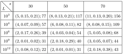
B Parameters choice

In Fig. 2 we show some possible values for (ℓ, ǫ1, ǫ2), for different security parameterss and circuit sizesL. In particular, we have chosen parameters that minimize the cost per gate – defined as 1 for any commitment or hash that needs to be transmitted per gate in the original circuit. The quantity we tried to minimize is therefore given by the cost expression

c= 5(ℓ+ 1)/(1−ǫ1) + 3(2ℓ+ 1)/(1−ǫ2) ,

under the constraint that P ≤2−s_{, with} _P _{as defined in Lemma 2. Every entry in the}

table is of the form (ℓ, ǫ1, ǫ2);c.

L s

30 50 70

103 (5,0.15,0.21); 77 (8,0.13,0.21); 117 (11,0.13,0.20); 156 104 (4,0.07,0.09); 57 (6,0.08,0.11); 82 (8,0.08,0.15); 109 106 ₍₂_,₀_.₁₇_,₀_._{26); 39 (4}_,₀_.₀₃_,₀_._{04); 54} ₍₅_,₀_.₀₅_,₀_._{08); 68}

109 ₍₂_,₀_.₀₁_,₀_._{02); 31 (2}_,₀_.₁₈_,₀_._{29); 40} ₍₃_,₀_.₀₅_,₀_._{07); 44}

1012 ₍₁_,₀_.₀₈_,₀_._{12); 22 (2}_,₀_.₀₁_,₀_._{01); 31} ₍₂_,₀_.₁₈_,₀_._{38); 43}

Figure 2.Parameters choice for different security parameterss and circuit sizesL, and resulting cost per gate.

To better understand the significance of the numbers in the table, it’s useful to recall that in the standard (passive secure) Yao protocol the cost per gate is 4, while in the protocol from [LPS08] the cost per gate is 4s, plus O(s2) commitments for every input gate.

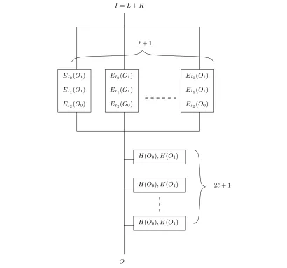
C A Replicated Gate

Fig. 3 illustrates the structure of a replicated gate with key checks.

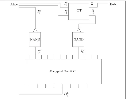
D Input/Output Structure

Fig. 4 illustrates how Alice and Bob provide their inputs to the garbled circuit, and how Alice gets her output.

E NOT gates for free

(20)

EI0(O1) EI1(O1) EI2(O0)

H(O0), H(O1)

EI0(O1) EI1(O1) EI2(O0)

ℓ+ 1

2ℓ+ 1

O I=L+R

Figure 3.The alignment ofℓ+ 1 NT gates and 2ℓ+ 1 KCs. Illustrated for the case where all components are correct.

In particular, if we have a set of keys Ki xi = K

i

0+xi∆, with i∈ {1, n}, and some

known integersa0, . . . , an∈N, we can compute a keyOy withy=Pn_i₌₁aixi+a0 in the following way: Alice opens the value S = open(Pn

i=1ai[K0i]−a0[∆]−[O0]), then Bob can computePn

i=1aiKxii −S=

Pn

i=1ai(K0i +xi∆)−Pni=1aiK0i+a0∆+O0 =Oy.

A special case of this is when n= 1, a0 = 1, a1 =−1, in which case we get a NOT gate. When we align two output wires with an input wire we can negate any of the inputs by setting the three values (a0, a1, a2) to: (0,1,1) for straight connection, (1,−1,1) to negate the left input, (1,1,−1) to negate the right input and (2,−1,−1) to negate both inputs.

F Sampling the Challenges using a Short Seed

(21)

Oky

Bob Alice

Encrypted CircuitC OT

b

Iw a

Iv b

Iv

0

Iv

1

NAND NAND

Figure 4.Alice inputs a bita into the input wireIi, while Bob inputs a bitbinto the input wire Ij. After the evaluation, Alice gets thek-th output key, encoding the bity.

Fix a subset I of the indices of the components and for each i∈I pick a challenge e(₀i) ∈ {0, . . . ,|E| −1}. If we picked each e(i) _{independently with Pr[}_e(i) ₌_e

0] = ǫ/|E| fore0∈ {0, . . . ,|E| −1}and Pr[e(i)=|E|] = 1−ǫ, then we would have that

Pr[∄i∈I(e(i) =e₀(i))] = (1−ǫ/|E|)|I| .

For simplicity we assume that the distribution (ǫ/|E|, ǫ/|E|, . . . , ǫ/|E|,1 −ǫ) can be sampled using a finite number of uniformly random bits, such that we can sample e = e(r) for a uniformly random r ∈ {0,1}c _{for a constant} _c_{. We can then sample all}

N elements e(i) _from _r _{∈ {0}_,_1}cN_{. If we instead use} _r _{which is} _δ_{-close to uniform on}

{0,1}cN, then

Pr[∄i∈I(e(i) =e₀(i))]≤(1−ǫ/|E|)|I|+δ . (1) In fact, it is enough that r isδ-almostk-wise independent on {0,1}cN _with_k_≥_c_|_I_{|, as}

the|I|values e(i) _{depend on at most} _c_|_I_|_{bits from}_r_.

To sample r we use a δ-almost k-wise independent sampler space sspc : {0,1}σ _→

{0,1}m_{, where for a uniformly random} _seed _S _{∈ {0}_,_1}σ _{the string} _r

I is δ-close to

uniformly random, wherer= sspc(S),I ⊂ {1, . . . , m},|I| ≤kandrI denotes the|I|-bit

string consisting ofr projected to coordinatesi∈I. We can e.g. use a construction from [AGHP92], where

(22)

We needk=O(s) andδ = 2−O(s)_{, and can safely assume that the bit length of}_r _{is less} that 22s

, giving us a seed length ofO(s), as desired.

The distribution of eache(i)isδ-close to the distribution (ǫ/|E|, ǫ/|E|, . . . , ǫ/|E|,1− ǫ), so the expected number of i for which e(i) ₌ _|_E_| _{is at least} _N₍₁₋_ǫ₎₋_{N δ}_{. We} always need to be left with N(1−ǫ) components. By pickingδ ≤2−s _{and by starting}

withN any small constant fraction larger than now (like 10%), we can by Chebychev’s inequality, ensure that the probability that we end up with N(1−ǫ) components not checked being at least 3₄. This very soon holding for large enough L and still with (1) holding for all I with|I| ≤k/c(we will soon fix k).

Now, letH denote the event that ∄i∈I(e(i)=e(₀i)) and let E denote the event that we are left with enough components (N(1−ǫ)). We have that Pr[H|E]≤Pr[H]/Pr[E]≤

4

3Pr[H]≤ 43((1−ǫ/|E|)|I|+δ).

For any β =O(s), let k=βc and δ = min(2−s,2−β−2). Then for all I with|I| ≤ β we have that

Pr[∄i∈I(e(i)6=e(₀i))]≤ 4

3(1−ǫ/|E|)

|I|_{+ 2}−β−1 _. ₍₂₎

By samplingS until it occurs that there are enough components left, we get enough components by using an expected 4₃ tries. Formally the UC model does not allow ex-pected poly-time protocols. We can handle this by terminating with some fixed C and e(i) if β + 1 tries failed. This occurs with probability at most 2−βi−1_{. Since (}4

3(1 − ǫ/|E|)|I|_{+ 2}−β−1_{) + 2}−β−1 ₌ 4

3(1−ǫ/|E|)|I|+ 2−β we get that Pr[∄i∈I(e(i)6=e(₀i))]≤ 4

3(1−ǫ/|E|)

|I|_{+ 2}−β _, ₍₃₎

as desired.

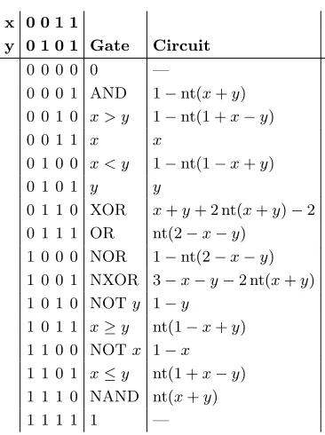
G How to Construct the Circuit

In Fig. 5 we implement the 16 binary Boolean functions using nt() gates and linear com-putation, achievable for free as explained in Appendix E. In this way we can implement any of the Boolean functions using just one nt() gate.

H Coin Flipping via OT

During the protocol we need to sample some random strings in a secure way. In particular we need to sample a random element h in the groupGand the seed S for thes-biased source of Appendix F.

Given that we are in the OT-hybrid model, we will present a way to reduce UC coin flipping to UC OT. The protocol allows the simulator to arbitrarily select the outcome of the coin flip.

The protocol is the following: To flip a random bit r Alice transfers two random strings A0 6= A1 ∈R {0,2s−1}. Bob retrieves one of the two strings at random, say

he picks b∈R{0,1} and he gets Ab. After the OT Alice sends a random bit a. Finally

Bob sends Alice the retrieved stringAb. The outcome of the protocol is the random bit

r=a⊕b. The protocol is intuitively secure, as the probability that Bob guessesA1−b is

negligible in s, and Alice gets no information at all about Bob’s bit bin the OT-hybrid model.

(23)

x 0 0 1 1

y 0 1 0 1 Gate Circuit 0 0 0 0 0 —

0 0 0 1 AND 1−nt(x+y) 0 0 1 0 x > y 1−nt(1 +x−y) 0 0 1 1 x x

0 1 0 0 x < y 1−nt(1−x+y) 0 1 0 1 y y

0 1 1 0 XOR x+y+ 2 nt(x+y)−2 0 1 1 1 OR nt(2−x−y)

1 0 0 0 NOR 1−nt(2−x−y) 1 0 0 1 NXOR 3−x−y−2 nt(x+y) 1 0 1 0 NOTy 1−y

1 0 1 1 x≥y nt(1−x+y) 1 1 0 0 NOTx 1−x

1 1 0 1 x≤y nt(1 +x−y) 1 1 1 0 NAND nt(x+y) 1 1 1 1 1 —

Figure 5.How to implement each of the binary Boolean functions using one NT gate.

wants to force the output to ber′_{: The simulator waits for Alice to send}_a_{and then he}

repliesb=a⊕r′. If Bob is malicious the simulator simply gets Bob’s choice b from the OT, and he replies with a=b⊕r′.

This protocol is composable, so if the parties need to sample ak-long bit-string, they just need to run the protocol ktime in parallel.

I Proof of Knowledge via OT

During the protocol Alice needs to prove in zero-knowledge that she knows an opening of the commitment [∆;r∆]. She doesn’t know the commitment trapdoor, so this defines

a value for∆.

Given that we are in the OT-hybrid model, we will present a way to reduce UC zero-knowledge proof of zero-knowledge to UC OT. The protocol allows the simulator to extract ∆.

The protocol is the following: Alice picks at random K0, r0 ∈R Zp. Define K1 = K0+∆, r1 =r0+r∆. Then Alice offers ((K0, r0),(K1, r1)) to the OT. Bob chooses a random bite∈R{0,1}and accepts ifKe, reis an opening of [K0]+e[∆]. They repeat the protocolstimes in parallel. Therefore, Alice cannot guess Bob’s choice with probability better than 2−s_{. Given that we are in the OT-hybrid model, If Alice is corrupted the}

simulator gets to see K0, K1, and therefore it can compute∆=K1−K0.

(24)

saves the tuples (ei, Keii,[K

i

0]) he gets during the protocol. Later, when he needs an input keyI_b(g)for an input gate g, he can ‘recycle’ those keys permuting them randomly and aligning them to the input wires. As shown in Appendix E this can be done even if b6=ei, using the NOT gate for free construction.

J Extracting ∆

We describe here what Bob should do if, for some internal gate g, he gets a set of keys O(g) _s.t _|O(g)_|_>_{1. In this case, except with negligible probability,}_O(g) ₌_{_O(g)

0 , O (g) 1 }. We call O_d(g), O(₁g₋)_d those two keys, as Bob doesn’t know which key is which. Clearly, ∆ = (−1)d(O(₁g₋)_d−O_d(g)), and therefore Bob needs to find d in order to find the right value of∆. The valuedis found as follows: For each input gateg′ where Bob is supposed to provide input, Bob takes the key O(_bg′)

i , which at this point we can assume correct.

Then he uses his input bit bi and the ℓ+ 1 KCs of g′ to determine the value of d: He

checks if there is a hash of O_b(g′)

i + (−1)

bi₍_O

1−d−Od) or O( g′₎

bi + (−1)

bi₍_O

d−O1−d) and

set d= 0 respectively d= 1 and he takes the majority vote.

K Extracting Most Component Generators with High Probability

We now describe an extractor which allows to extract generators for most components when Bob is honest and accepts the checks. We note that the extractor rewinds the environment. Therefore the extractor is not a sub-routine which can be run by the simulator in a proof in the UC model. This is not a problem, as this is not the intended use. Our UC simulator does not run this extraction. The fact that some imaginary algorithm X could have rewound the environment and the entire execution to produce generators will be used to analyze the simulator, not construct it.

In a bit more details, if Alice is corrupted and Bob is honest, then for all adversaries and all environments we consider an extractor X which can be run on the terminal global state of the environment, the adversary and the execution of the protocol to try to extract components generators for the components used by Alice and Bob. By the

augmented execution we mean: First run the protocol with the given environment and adversary until it terminates, and thenif Bob accepts the checks,then run the extractor on the terminal global state of the environment, the adversary and the execution of the protocol. The extractor X has the following properties:

– The augmented execution is expected poly-time.

– The extractor in the augmented execution computes generators for all components except a few, where the exactly number of missing components relates to the prob-ability the Bob accepts.

We start by some technical definitions and lemmas.

Definition 1. Given a poly-time binary relation R we call (E,reply,accept) a simple proof of knowledge for R if E is a finite set and accept(x, e,reply(w, e)) = 1 for all

(25)

The check we do for NT gates and KCs are clearly simple proofs of knowledge (see Appendix L), with the witness being the generator of the components and the relation being that the generator gives rise to the component.

For a simple proof of knowledge we are interested in the following protocol for gener-ating proved instances, parametrized by some constant ǫ∈(0,1) and integers δ, L∈N. 1. The prover P sends Linstancesx1, . . . , xL _{for which it knows witnesses}_w1_{, . . . , w}L_.

2. The verifier V selects a random subsetC of the instances, and sendsei =|E|fori6∈ C. For each i∈C,V in addition sends a random challengeei_∈_E ₌_{0_{, . . . ,}_|_E_{| −}_1}.

3. For each ei 6=|E|,P sends zi= reply(wi, ei) to P.

4. V checks that verify(xi_{, e, z}i_{) = 1 for all}_ei ₆₌_|_E_{|. If so, the output is (}_accept!_,_{_xi_} ei₌_|_E_|).

Otherwise, the output is reject!.

We pick the challenges ei such that for any fixed subsetI with |I| ≤δ and for fixed challenges ei

0 ∈E fori∈I, it holds that Pr[∄i∈I(ei 6=ei₀)]≤ 4

3(1−ǫ/|E|)

|I|_{+ 2}−δ _.

For each β ∈ {1, . . . , δ−3} we describe an extractor Xβ. It can be run on a state

of the protocol execution right after the verifier accepted the checks, and it will try to extract witnesses forL−β of the instances.

1. For each xi _{and each} _e _∈ _E _{for which no correct reply} _zi

e is stored: rewind the

execution to where the challenges are sent and send a random seed S giving rise to ei ₌_e_{, run the execution to receive some}_zi

e, and store it if it is correct. Note the an

independent rewind and rerun is used for each such (xi_{, e}_{), meaning that the step}

can include as many as L|E|reruns.

2. If for all but β of the instances correct replies zei are stored for all e ∈ E, then

compute witnesses for all theseL−β instances and terminate. Otherwise, go to the above step.

By the β-augmented protocol we mean the following: First run the protocol until V accepts or rejects. If V rejected then stop. Otherwise, run Xβ on the trace of the

execution to extractL−β witnesses.

Lemma 2. If β ≤δ−3 and the probability thatV accepts the proof is ≥2(1−ǫ|E|−1)β_, then the expected running time of the β-augmented protocol is polynomial.

Proof. Fix a state of the protocol execution right after Step 1 is executed, i.e., right after the instances are sent. We make some definitions relative to such a state.

For an index i∈ {1, . . . , L} and a challenge e∈E we define Accept(i, e)∈ [0,1] to be the probability that the prover replies with a correctzi _{if the verifier sends a random}

seed S giving rise toei ₌_e_{. For each} _i _{we let}_ǫi _{be an element} _e_∈_E _{which minimizes}

Accept(i, e) and we let Accept(i) = Accept(i, ǫi).

For each β ∈ {1, . . . , L} we can pick Aβ such that there exists Aβ ⊆ {1, . . . , L} for

which |Aβ| = L−β and Accept(i) ≥Aβ for i ∈ Aβ and Accept(i) ≤ Aβ for i 6∈ Aβ.

Think ofAβ as the largest accept probability we can pick such that at mostβ instances

LEGO for Two Party Secure Computation

LEGO for Two Party Secure Computation

Contents