Vol. 5, Special Issue 8, May 2016
Optimization of Cutting Tool Life Parameters
By Application of Taguchi Method on a
Verticalmilling Machine
A.Manigandan 1, D.Lerin Jose2, S.Mathava Arun 3, P.Ravishankar 4, V.Sakthivel 5
Assistant Professor, Department of Mechanical Engineering, TRP Engineering College, Tiruchirapalli, India1
UG Scholars, Department of Mechanical Engineering, TRP Engineering College, Tiruchirapalli, India 2,3,4,5
ABSTRACT: Our work focuses on the optimization of cutting tool life of a Vertical milling machine and end milling operation is performed on it by using Cubic Boron Nitride (CBN) as the cutting tool material and En8 steel (HRC 46) as work piece material to predict the tool life. End mills are used in tracer controlled profile milling operations. They are employed for making deep grooves in base parts, profile recesses, steps, etc. End mills can be used on horizontal milling machine, but it is better to use them on vertical milling machine. Their diameter varies from about 3mm to 50mm. They are usually made from high speed steel (HSS) or carbide, and have one or more flutes. They are the most common tool used in a vertical mill. The input of the model consists of feed rate, cutting speed and depth of the cut while the output from the model is the tool life which is calculated by Taylor’s tool life equation. This research is to test the collecting data by Taguchi method. The model is validated through a comparison of the experimental values with their predicted counterparts. The optimization of the tool life is studied to compare the relationship of the parameters involved. The result of the experimental optimization shows that depth of cut was the only parameter found to be significant. The experimental optimization also shows that the predicted values and calculated values are very close, that clearly indicates that the developed model can be used to reduce the cost of machining.
I. INTRODUCTION
MACHINING
Machining is any of various processes in which a piece of raw material is cut into a desired final shape and size by a controlled material-removal process. The processes that have this common theme, controlled material removal, are today collectively known as subtractive manufacturing, in distinction from processes of controlled material addition, which are known as additive manufacturing. Exactly what the "controlled" part of the definition implies can vary, but it almost always implies the use of machine tools (in addition to just power tools and hand tools).Machining is a part of the manufacture of many metal products, but it can also be used on materials such as wood, plastic, ceramic, and composites. A person who specializes in machining is called a machinist. A room, building, or company where machining is done is called a machine shop. Machining can be a business, a hobby, or both. Much of modern day machining is carried out by computer numerical control in which computers are used to control the movement and operation of the mills, lathes, and other cutting machines.
TYPES OF CUTTING TOOL
Single point tool; and
Multiple-cutting-edge tool
SINGLE POINT CUTTING TOOL
A single point tool has one cutting edge and is used for turning, boreing and planing. During machining, the point of the tool penetrates below the original work surface of the workpart. The point is sometimes rounded to a certain radius, called the nose radius.
MULTIPLE CUTTING EDGE TOOL
Multiple-cutting-edge tools have more than one cutting edge and usually achieve their motion relative to the work part by rotating. Drilling and milling uses rotating multiple-cutting-edge tools. Although the shapes of these tools are different from a single-point tool, many elements of tool geometry are similar
II. LITERATURE REVIEW
Luo et al.(2005) “Modeling flank wear of carbide tool insert in metal cutting”In this paper theoretical and experimental studies are carried out to investigate the intrinsic relationship between tool flank wear and operational conditions in metal cutting processes using carbide cutting inserts. A new flank wear rate model, which combines cutting mechanics simulation and an empirical model, is developed to predict tool flank wear land width. A set of tool wear cutting tests using hard metal coated carbide cutting inserts are performed under different operational conditions. The wear of the cutting inset is evaluated and recorded using Zygo New View 5000 microscope. The results of the experimental studies indicate that cutting speed has a more dramatic effect on tool life than feed rate. The wear constants in the proposed wear rate model are determined based on the machining data and simulation results. A good agreements between the predicted and measured tool flank wear land width show that the developed tool wear model
can accurately predict tool flank wear to some extent.Ishan B Shah, Kishore. R. Gawande(2012) “Optimization of
Vol. 5, Special Issue 8, May 2016
contributions of parameters as quantified in the S/N pooled ANOVA envisage that the relative power of feed (8.78 %) in controlling variationand mean tool life is significantly smaller than that of the cutting speed (34.89 %) and depth of cut (25.80 %). The predicted optimum tool life is 20.19 min. The results have been validated by the confirmation
experiments.Anjan Kumar Kakati, M. Chandrasekaran, AmitavaMandal, and Amit Kumar Singh(2011)
“Prediction of Optimum Cutting Parameters to obtain Desired Surface in Finish Pass end Milling of Aluminium Alloy with Carbide Tool using Artificial Neural Network”End milling process is one of the common metal cutting operations used for machining parts in manufacturing industry. It is usually performed at the final stage in manufacturing a product and surface roughness of the produced job plays an important role. In general, the surface roughness affects wear resistance, ductility, tensile, fatigue strength, etc., for machined parts and cannot be neglected in design. In the present work an experimental investigation of end milling of aluminium alloy with carbide tool is carried out and the effect of different cuttingparameters on the response are studied with three-dimensional surface plots. An artificial neural network (ANN) is used to establish the relationship between the surface roughness and the input cutting parameters (i.e., spindle speed, feed, and depth of cut). The Matlab ANN toolbox works on feed forward back propagation algorithm is used for modeling purpose. 3-12-1 network structure having minimum average prediction error found as best network architecture for predicting surface roughness value. The network predicts surface roughness for unseen data and found that the result/prediction is better. For desired surface finish of the component to be produced there are many different combination of cutting parameters are available. The optimum cutting parameter for obtaining desiredsurface finish, to maximize tool life is predicted. The methodology is demonstrated, number of
problems are solved and algorithm is coded in Matlab.Wen-Hsiang Lai(2000) “Modeling of Cutting Forces in End
Milling operations”According to previous research of dynamic end milling models, the instantaneous dynamic radii on every cutting position affects the cutting forces directly since the simulated forces are proportional to the chip thickness, and the chip thickness is a function of dynamic radii and feed rate. With the concept of flute engagement introduced, it is important to discuss it with respect to radial and axial depths of cut because the length of the engaged flutes is affected by factors in the axial feed and rotational directions. Radial and axial depths of cut affect the “contact area”, which is the area that a cutter contacts with the work piece. When radial and axial depths of cut increase, the cutting forces also increase since the engaged flute lengths are increased. Therefore, in order to have a clearer idea of the milling forces, the influences of dynamic radii, cutting feed rate, and radial and axial depths of cut are discussed in this paper.
III. METHODOLOGY
TAGUCHI METHOD
Taguchi methods are statistical methods developed by Genichi Taguchi to improve the quality of manufactured goods. Professional statisticians have welcomed the goals and improvements brought about by Taguchi methods particularly by Taguchi's development of designs for studying variation, but have criticized the inefficiency of some of Taguchi's proposals.
Taguchi's work includes three principal contributions to statistics:
A specific loss function
The philosophy of off-line quality control; and
Innovations in the design of experiments.
Every experimenter has to plan and conduct experiments to obtain enough and relevant data so that he can infer the science behind the observed phenomenon. He can do so by,
TRIAL AND ERROR APPROACH
DESIGN OF EXPERIMENTS
A well planned set of experiments, in which all parameters of interest are varied over a specified range, is a much better approach to obtain systematic data. Mathematically speaking, such a complete set of experiments ought to give desired results. Usually the number of experiments and resources required are prohibitively large. Often the experimenter decides to perform a subset of the complete set of experiments to save on time and money. However, it does not easily lend itself to understanding of science behind the phenomenon. The analysis is not very easy and thus effects of various parameters on the observed data are not readily apparent. In many cases, particularly those in which some optimization is required, the method does not point to the BEST settings of parameters.
TAGUCHI PRINCIPLE
Dr. Taguchi of Nippon Telephones and Telegraph Company, Japan has developed a method based on " orthogonal array " experiments which gives much reduced “variance " for the experiment with " optimum settings " of control parameters. "Orthogonal Arrays" (OA) provide a set of well balanced (minimum) experiments and Dr. Taguchi's Signal-to-Noise ratios (S/N), which are log functions of desired output, serve as objective functions for optimization, help in data analysis and prediction of optimum results.
Taguchi Method treats optimization problems in two categories,
STATIC PROBLEMS
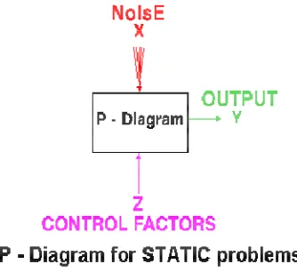
Generally, a process to be optimized has several control factors which directly decide the target or desired value of the output. The optimization then involves determining the best control factor levels so that the output is at the target value. Such a problem is called as a "STATIC PROBLEM".
This is best explained using a P-Diagram which is shown below ("P" stands for Process or Product). Noise is shown to be present in the process but should have no effect on the output! This is the primary aim of the Taguchi experiments - to minimize variations in output even though noise is present in the process. The process is then said to have become ROBUST.
Fig 5.1 P-Diagram for Static problems DYNAMIC PROBLEMS
If the product to be optimized has a signal input that directly decides the output, the optimization involves determining the best control factor levels so that the “input signal / output” ratio is closest to the desired relationship. Such a problem is called as a “DYNAMIC PROBLEM”.
Vol. 5, Special Issue 8, May 2016
Fig 5.2 P-Diagram for Dynamic problems
-STEPS IN TAGUCHI METHODOLOGY
Taguchi method is a scientifically disciplined mechanism for evaluating and implementing improvements in products, processes, materials, equipment, and facilities. These improvements are aimed at improving the desired characteristics and simultaneously reducing the number of defects by studying the key variables controlling the process and optimizing the procedures or design to yield the best results.
The method is applicable over a wide range of engineering fields that include processes that manufacture raw materials, sub systems, products for professional and consumer markets. In fact, the method can be applied to any process be it engineering fabrication, computer-aided-design, banking and service sectors etc. Taguchi method is useful for 'tuning' a given process for 'best' results.
Taguchi proposed a standard 8-step procedure for applying his method for optimizing any process, Step-1: Identify the main function, side effects, and failure mode
Step-2: Identify the noise factors, testing conditions, and quality characteristics Step-3: Identify the objective function to be optimized
Step-4: Identify the control factors and their levels Step-5: Select the orthogonal array matrix experiment Step-6: Conduct the matrix experiment
Step-7: Analyze the data, predict the optimum levels and performance Step-8: Perform the verification experiment and plan the future action
ORTHOGONAL ARRAY
In mathematics, in the area of combinatorial designs, an orthogonal array is a "table" (array) whose entries come from a fixed finite set of symbols (typically, {1,2,...,n}), arranged in such a way that there is an integer t so that for every selection of t columns of the table, all ordered t-tuples of the symbols, formed by taking the entries in each row restricted to these columns, appear the same number of times. The number t is called the strength of the orthogonal array. Here is a simple example of an orthogonal array with symbol set {1,2}:Notice that the four ordered pairs (2-tuples) formed by the rows restricted to the first and third columns, namely (1,1), (2,1), (1,2) and (2,2) are all the possible ordered pairs of the two element set and each appears exactly once. The second and third columns would give, (1,1), (2,1), (2,2) and (1,2); again, all possible ordered pairs each appearing once. The same statement would hold had the first and second columns been used. This is thus an orthogonal array of strength two.
Orthogonal arrays generalize the idea of mutually orthogonal latin squares in a tabular form. These arrays have many connections to other combinatorial designs and have applications in the statistical design of experiments, coding theory, cryptography and various types of software testing.
DEFINITION
A t-(v,k,λ) orthogonal array (t ≤ k) is a λvt × k array whose entries are chosen from a set X with v points such that in every subset of t columns of the array, every t-tuple of points of X appears in exactly λ rows.
1 1 1
2 2 1
1 2 2
In this formal definition, provision is made for repetition of the t-tuples (λ is the number of repeats) and the number of rows is determined by the other parameters.
In many applications these parameters are given the following names: v is the number of levels,
k is the number of factors,
λvt is the number of experimental runs, t is the strength, and
λ is the index.
An orthogonal array is simple if it does not contain any repeated rows.
An orthogonal array is linear if X is a finite field of order q, Fq (q a prime power) and the rows of the array form a subspace of the vector space (Fq)k.[1]
Every linear orthogonal array is simple. SELECTION OF ORTHOGONAL ARRAY
In Taguchi method-based design of experiments, to select an appropriate orthogonal array for experimentation, the total degrees of freedom (DOF) needs to be computed. The DOF is defined as the number of comparisons between machining parameters that need to be made to determine, which level is better and specifically how much better it is. For example, a three-level machining parameter has two DOF. The DOF associated with interaction between two machining parameters are given by the product of the DOF for the two machining Parameters. In the present study, interactions between the three machining parameters will be considered. Therefore, there are 18 DOF owing to three three-level independent parameters. In this study, a L27 orthogonal array has been used because it has 26 DOF, which is higher than 18 DOF of the chosen independent parameters and their interactions. It can accommodate seven three level parameters and three interactions at most.
Cutting Parameters
Symbol Cutting
Parameters
Level 1 Level 2 Level 3
V Cutting Speed
(rev/min)
200 270 340
F Feed
(mm/min)
0.2 0.15 0.25
D Depth of cut
(mm)
0.6 0.8 1.0
Experimental Data
Trial No. Cutting Speed
(rev/min)
Feed (mm/min)
Depth of cut (mm)
1 200 40 0.6
2 200 40 0.8
3 200 40 1.0
4 200 30 0.6
5 200 30 0.8
6 200 30 1.0
Vol. 5, Special Issue 8, May 2016
8 200 50 0.8
9 200 50 1.0
10 270 54 0.6
11 270 54 0.8
12 270 54 1.0
13 270 40.5 0.6
14 270 40.5 0.8
15 270 40.5 1.0
16 270 67.5 0.6
17 270 67.5 0.8
18 270 67.5 1.0
19 340 68 0.6
20 340 68 0.8
21 340 68 1.0
22 340 51 0.6
23 340 51 0.8
24 340 51 1.0
25 340 85 0.6
26 340 85 0.8
27 340 85 1.0
V. RESULT AND DISCUSSION
FORMULAE
Now tool life can be calculated by using extended Taylor’s equation for above shown practical range of cutting parameters and results being tabulated manually.
Where,
T = Tool life in min, f = feed in mm per revolution, d = depth of cut in mm
n = Tool constant for CBN– 0.6(from tool manufacturer’s data book) n1= feed exponent constant – 0.21 (from tool manufacturer’s data book)
n2 =depth of cut exponent constant- 0.26(from tool manufacturer’s data book) C= constant- 3000(from tool manufacturer’s data book)
6.2 CALCULATION OF TOOL LIFE i). T = (C ) /( V x f x n1 x d x n2 )1/n T=(3000)/(200x40x0.6x0.21x0.26)1/0.6 T=31 mins
Results
Trial No. Cutting Speed
(rev/min)
Feed (mm/min)
Depth of cut (mm)
Tool Life (min)
Machining Time (sec)
1 200 40 0.6 31 150
2 200 40 0.8 28 150
3 200 40 1.0 25 150
4 200 30 0.6 35 200
5 200 30 0.8 30 200
6 200 30 1.0 28 200
7 200 50 0.6 29 120
8 200 50 0.8 25 120
9 200 50 1.0 23 120
10 270 54 0.6 17 111.11
11 270 54 0.8 15 111.11
12 270 54 1.0 14 111.11
13 270 40.5 0.6 19 148.15
14 270 40.5 0.8 17 148.15
15 270 40.5 1.0 15 148.15
16 270 67.5 0.6 16 88.89
17 270 67.5 0.8 14 88.89
18 270 67.5 1.0 12 88.89
19 340 68 0.6 11 88.24
20 340 68 0.8 9 88.24
Vol. 5, Special Issue 8, May 2016
22 340 51 0.6 12 117.65
23 340 51 0.8 10 117.65
24 340 51 1.0 9 117.65
25 340 85 0.6 10 70.58
26 340 85 0.8 9 70.58
27 340 85 1.0 8 70.58
0 50 100 150 200 250
40 30 50 54 40.5 67.5 68 51 85
Machining Time
machining speed
Graph 6.2 Tool Life Vs Depth of Cut
Graph 6.3 Tool Life Vs Feed
VI. CONCLUSION
As There are numbers of Parameters which affect the Tool life of end milling Cutters of vertical milling machine, According to present Work conditions and necessary Experiment set up being situated in an industry cutting parameters being chosen for experiment. Mainly Three cutting parameters named Cutting speed, Depth of cut, Feed may be selected and optimize these three parameters using taguchi method. In this case The Experimental results demonstrate that the cutting speed and depth of cut are the main parameters that Influence the tool life of end mill cutters of vertical milling machine. The tool life can be improved simultaneous through taguchi method approach instead of using Engineering judgment. The confirmation experiments were conducted to verify optimal cutting parameters.
Experimental results show that in milling operations, Use of Low depth of cut, low cutting speed and low feed rate and high machining time are recommended to obtain better Tool life for the specific Range at,
Speed (V) = 200 rpm Depth of cut (d) = 0.6 mm Feed rate (f) = 30 mm/min Tool life=31mins
Vol. 5, Special Issue 8, May 2016
REFERENCES
[1] Choudhury, M.A. El-Baradie,’’ Tool-life prediction model by design of experiments for turning high strength steel (290 BHN).” Journal of Materials Processing Technology 77 (1998) 319–326
[2] Keun Park Jong-Ho Ahn, “Design of experiment considering two-way interactions and its application to injection molding processes with numerical analysis.” Journal of Materials Processing Technology 146 (2004) 221–227
[3] ChristelPierlot, Lech Pawlowski, MurielBigan, Pierre Chagnon, “Design of experiments in thermal spraying: A review”. Surface & Coatings Technology 202 (2008) 4483–4490.
[4] Dong-Woo Kim, Myeong-Woo Cho, Tae-Il Seo, Eung-SugLee,”Application of Design of Experiment Method for Thrust Force Minimization in Step-feed Micro Drilling.’’ Sensors 2008, 8, 211-221
[5] IlhanAsiltürk, HarunAkkus,” Determining the effect of cutting parameters on surface roughness in hard turning using the Taguchi method.” Science direct Measurement 44 (2011) 1697–1704
[6] Yung-Kuang Yang, Ming-Tsan Chuang, Show-Shyan Lin, ” Optimization of dry machining parameters for high-purity graphite in end milling process via design of experiments methods.”, Journal of Materials Processing Technology 209 (2009) 4395–4400.