DEEP NEURAL CLASSIFICATION AND LOGIT REGRESSION BASED ENERGY EFFICIENT ROUTING IN WIRELESS SENSOR NETWORK

2041

AN EFFICIENT TECHNIQUE FOR CLUSTER NUMBER

PREDICTION IN GRAPH CLUSTERING USING NULLITY OF

LAPLACIAN MATRIX

1_{IMELDA ATASTINA,} 1_{BENHARD SITOHANG,} 1_{G.A.PUTRI SAPTAWATI,} 2_VERONICA

S.MOERTINI

1_{Institut Teknologi Bandung, Jl.Ganesha no.10 Bandung 40132, Indonesia}

2 _{Chatolic Parahyangan University, Jl.Ciumbuleuit no.11 Bandung 41311,Indonesia}

E-mail: [email protected]

ABSTRACT

Clustering graph dataset representing users’ interactions can be used to detect groups or communities. Many existing graph clustering algorithms require an initial cluster number. The closer the initial cluster numbers to the real or final ones, the faster the algorithm will converge. Hence, finding the right initial cluster number is important for increasing the efficiency of the algorithms. This research proposes a novel technique for computing the initial cluster number using the nullity of the Laplacian Matrix of Adjacency Matrix. The fact that nullity relates to the properties of the eigenvalues in the Laplacian matrix of a connected component is used to predict the best cluster numbers. By using this technique, trial and error experiments for finding the right clusters is no longer needed. The experiment results using artificial and real dataset and modularity values (for measuring the clusters quality) showed that our proposed technique is efficient in finding initial cluster numbers, which is also the real best cluster numbers.

Keywords: Estimating the Number of Clusters, Nullity, Laplacian Matrix, Adjacency Matrix, Graph Clustering

1. INTRODUCTION

The study of graph clustering has been impressive for about two decades because various fields or businesses can utilize the results of graph clustering. The existence of graph clustering algorithm has driven some studies to improve its performance, such as how to increase the running time of the algorithm [1] and how to deal with big data using spectral graph clustering [2]. Furthermore, one of the important problems related to running time is to predict the amount of the clusters consisting of a graph. Predicting the number of the clusters is an essential step in running a graph clustering algorithm because the prediction of clusters number not only will influence the time to do graph clustering, but also the quality clustering result. It is understood, the closer initial value prediction to the best solution will lead to faster time processing and good cluster quality. So, it will be beneficial when determining the number of clusters

in a graph can be done in one step without the need to compare or try various possibilities for the number of clusters.

2042 number of vertices and edges, so predicting the number of clusters contained in a graph needs a thorough analysis. Graph visualization or simple statistic inadequate to give an early overview to help the user to predict the number of subgraphs or clusters in a graph. Graph Clustering Using Dirichlet Process Mixture Model (DPMM) shows DPMM failed to estimate the number of the clusters for a large graph because there are too many possibilities that can be tried as the number of clusters.[6], [7].

In data clustering task, there are also several methods have been proposed to determine the number of clusters. For instance, Salvador and Chan proposed Knee Method [8], Hu and Xu proposed an iterative method using Expectation Maximization to determine the number of groups [9], Tibhsirani proposed the gap statistic [10] and Fujita introduced the slope statistic [11] to determine the number of clusters. Because of the similarities between graph clustering and data clustering task, there is an idea to adapt the methods to determine the number of clusters in the graph clustering task. However, it is required some studies to adjust the technique in graph clustering, and to the best of our knowledge, no research has been carried out regarding this matter. Besides, there is a similarity of those methods, that the algorithms should be tried in various values of the number of the clusters, comparing the quality cluster value and finally choose the best number of clusters related to the maximum quality cluster value. That technique is indeed less efficient.

This study proposed utilizing the nullity of the Laplacian Matrix of the graph showing a simple method and solid foundation, to estimate the number of clusters. Nullity is an algebra term states how many times a zero value appears as an eigenvalue of a matrix. So far nullity is only known as one of the properties of the matrix. It is not found out how this nullity was exploited before. However, the intended nullity in this study is the nullity value of the Laplacian matrix formed from the adjacency matrix of a graph. This research showed the concept and illustration of how nullity can be used to predict the number of the cluster in a graph. Also, it exhibited elaboration result utilizing the nullity of the Laplacian Matrix of the graph, thus the user gets an idea how to use the nullity value in predicting the number of clusters and how to use it appropriately to obtain optimum cluster results. An additional finding from the research showed that the best cluster

number by comparing all possible number of clusters is an improper method.

The rest of the paper will consist of the property of the graph and the rationale of the proposed method in section 2, the proposed algorithm in section 3, the experiment and the result in section 4, some discussion and insight related to the experiment result in section 5, and section 6 is the conclusion and future work.

2. THE PROPERTY OF A GRAPH

A Graph is a diagram consisting of vertices and/or edge. The layout can be used to represent the relation between two or more objects by attaching an edge between relational objects. For example, communication relationships that occur between phone account numbers, friendship relationships or interactions between accounts in social media, flight schedules, items purchased together in a store, and so on. A Graph is a simple representation. Nonetheless, a graph can contain a variety of useful information. One of the vital information in a graph is the existence of groups or communities [12].

Knowledge of a community is valuable information in a business. For instance, based on data on social media interaction it can be found the group of people who love golf, and then it will be useful when the businessman who sells various golf

2043 equipment is offering the goods to the community. Therefore, acquiring knowledge or information in the form of a community is essential. This information can be obtained by doing graph clustering.

2.1 Graph Clustering

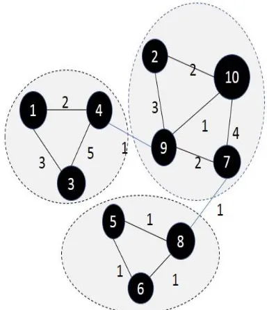
Graph clustering is one of the techniques to process the graph dataset to detect groups or communities contained in a graph [13]. The purpose of graph clustering is to group nodes that have strong relationships and similarities between vertices. Strong relationships can be seen from the edge weights or the number of equal neighbors, whereas the similarity between vertices in graph clustering is seen from the same number of friends. Figure 1 is an illustration of graph clustering result. The illustration depicts the result of graph clustering implementation of a graph that consists of ten nodes, so that the vertices in the graph can be grouped into three clusters. The first cluster consists of vertex 1,3 and 4, second cluster consists of vertex 2,7,9 and 10, and the last cluster consists of vertex 5,6, and 8.

One of the most popular and often used algorithms for graph clustering is the Graph Spectral Clustering Algorithm because the algorithm is easy to implement and robust [1], [2]. Graph Spectral Clustering algorithm is developed based on the knowledge that a graph can be represented in the form of an adjacency matrix. Therefore, the algebraic properties of a matrix can be used to understand the characteristics of the graph. The theory discussing how to interpret the characteristics of a graph through its adjacency matrix is known as Graph Spectral Theory [14] . Based on the theory, the user works merely with the adjacency matrix of the graph. Thus, information or knowledge related to the graph can be inferred based on the result of processing an adjacent matrix.

The essential steps in the Graph Spectral Clustering algorithm are defining the adjacent matrix of a graph, then mapping the adjacent matrix into a Laplacian matrix, and inputting the rows of the Laplacian matrix into the Means algorithm. K-Means algorithm is the commonly used data clustering algorithm. The Graph Spectral Algorithm can be written as follows:

Input : A ( adjacency Matrix of graph G), k (number of clusters)

Output : 𝐶 ; 𝑗 1,2,3, … , 𝑘 ; 𝐶= Cluster – j Steps :

1. Create Laplacian Matrix of G 𝐿

2. Solve det 𝜆𝐼 𝐿

3. Compute k eigenvector of 𝐿 that related to the k largest eigenvalue

4. Create matrix 𝑌 , where each column of y is a vector from the result of step 4 5. Cluster the row of matrix 𝑌 using the k

-means algorithm, with determined k

Mapping the adjacency matrix into a Laplacian matrix causes as if the relationship between vertices to be disappearing, and the Laplacian matrix rows are like ordinary data (not graph), where each row represents an object in the Laplacian matrix with features corresponding to the columns of the Laplacian matrix. Therefore the K-Means algorithm can be directly used for clustering the rows of the Laplacian matrix [4].

2.2 The Nullity of Laplacian Matrix

In addition to the Laplacian matrix properties of the adjacency matrix of a graph, one of the important theorems of the Spectral Graph Theory is the theorem relating to the nature of connectivity of a graph. The theorem states, the nullity value of a Laplacian matrix of an adjacency matrix of a graph is equal to the number of connected components in a graph [5], [14]. The nullity is a digit that denotes the number of zero appears as an eigenvalue of a matrix. The eigenvalue itself can be obtained by finding the solution of the following equation

𝒅𝒆𝒕 𝝀𝑰 𝑴 𝟎 (1)

where λ = eigenvalues, 𝐼 = identity matrix, and M = matrix. It should be noted that the nullity value used to predict the number of clusters contained in graph

𝐺 is the nullity of the Laplacian matrix of the adjacent matrix of a graph. So, the steps to calculate the nullity as a conjecture of the number of clusters in a graph is, as follows:

1. Create

𝐴

2. Calculate

𝐿

𝐿

𝐷 𝐴

where

𝐷

𝑑

𝑑

∑ 𝑎 ; 𝑎

∈ 𝐴

3. Find the eigenvalues by solving the equation

det 𝜆𝐼

𝐿

0

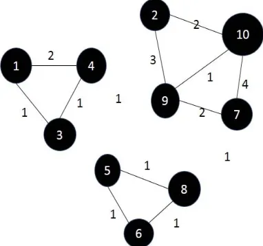
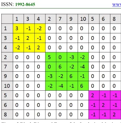
2044 The nullity of the Laplacian matrix of the graph can be used as a prediction tools because it relates to the properties of the eigenvalues of the Laplacian matrix of a connected component always zero and symmetric. So, if a graph contains several connected components, then the Laplacian matrix of the adjacency matrix of the graph will consist of several blocks of diagonal matrices, where each matrix block is symmetric and the eigenvalues of the block is zero. For example, suppose that there is a graph G consisting of 10 vertices and containing three connected components as described in Figure 2, and its adjacency matrix as in Figure 3, and the Laplacian matrix of the adjacency matrix of G is obtained as shown in Figure 4.

Figure 2 Graph G consists of three Connected Components

Notice the Laplacian matrix can be arranged in the form of a block diagonal matrix, such as described in Fig. 5, in which the eigenvalues of each diagonal block are zero. In addition, each diagonal block is related to the connected components contained in the graph.

This study focused on elaborating the theorem as a tool to predict the number of clusters contained in a graph. The research is also done by considering the clustering method proposed by Newman and Girvan.

Figure 3 The Adjacency Matrix of the Graph G

Whereas, Newman and Girvan proposed the graph clustering method, by removing the edges with high betweenness values in the graph [15], [16]. Edge betweenness is a connector that connects two subgraphs. So, when the edge betweenness is removed, then the graph will only consist of connected components or clusters. It can be concluded counting the number of connected components is equal to count the number of clusters in the graph. So, according to the graph theorem of connectivity, it can be used the nullity as estimation or prediction of the number of clusters.

2045 Figure 5 Block Diagonal Form of the Laplacian Matrix of

Graph G

3. GRAPH CLUSTERING ALGORITHM

USING NULLITY OF LAPLACIAN MATRIX ASTHEPREDICTORNUMBEROFCLUSTER

The proposed algorithm is a combination of nullity value calculation algorithm with graph spectral clustering algorithm. This study recommended to use counting the nullity of the Laplacian Matrix of the graph as the estimation of the number of the cluster as stated in Table 1.

Table 1 Modified Graph Spectral Clustering Algorithm

Input : A (adjacency matrix of G) Output: Cj, j =1, 2,…,k ; Cj = Cluster-j

Steps:

1. Create 𝐿 2. Solve det 𝜆𝐼 𝐿 3. Count the nullity (k)

4. Compute k eigenvector of 𝐿 that related to

the k largest eigenvalue

5. Create matrix 𝑌 , where each column of y is a vector from the result of step 4

6. Cluster the row of matrix 𝑌 using the k

-means algorithm, with determined k

The original Graph Spectral Clustering algorithm excludes the step counting the nullity as mention in step 2 and step 3 in Table 1. Thus, the input is given to the Modified Spectral Graph Clustering Algorithm only the adjacency matrix. A user does not need to input the conjectured value of the cluster number. So far, graph spectral clustering algorithm is started by giving a “trial and error” number of the cluster until the user assume the

modularity value obtained is satisfactory or manually comparing one by one the possible number of cluster values on a graph resulting in the greatest modularity values. Implementing both methods will, of course, lead to a longer time processing compared to calculating the nullity value, notably when the number of vertices is large. Also, mainly comparing the quality of clusters resulted from different clusters number is not an appropriate method for determining the number of clusters that produce the highest quality clusters, if a user does not compare all possible initial value combinations. This condition will be explained further in the discussion section.

4. EXPERIMENTS

Experiments were conducted to elaborate on the performance of nullity in determining the best clusters number. Therefore, testing was conducted on two data groups, namely artificial data, and real-world data. The performance was measured using modularity and time in seconds. Modularity is a parameter to measure the quality of the graph clustering result, whereas the range of modularity is between -1 and 1. A small value of modularity shows the structure of the cluster is weak, while the higher modularity shows, the stronger structure of the group. To calculate the modularity value, we use equation (4).

𝑄 ∑ 𝑒 𝑎 (4)

Where 𝑄 = modularity value, 𝑒 = weight ratio of the edges connecting vertices in cluster-i and cluster-j to all edge in the original graph and 𝑎 ∑ 𝑒 .

4.1 Dataset

2046 The real-world data consists of several graphs, that is formed based on the actual transactions. These graphs have various characteristics, and the descriptions can be seen in Table 3. We choose different size and types such as directed vs. undirected and weighted vs. unweighted graph, to investigate the performance of estimating the number of clusters using nullity of Laplacian Matrix of the graph. Most of the data are taken from http://konect.uni-koblenz.de(*), and from www.snap.com.

Table 2 List of Artificial Dataset

Name #Node #Edge # Clusters

1

Graph32 3 1 2

2

Graph421 4 3 2

3

Graph421_weight 4 3 2

4

Graph422 4 2 2

5

Graph102 10 13 2

6

Graph103 10 11 3

7

Graph103_weight 10 11 3

8

Graph104 10 8 4

4.2 Experiment Scenario

As explained on previous sections, the goal of the experiment is to understand the performance of the nullity value in predicting the number of

clusters in a graph. Thus, it was designed into some scenarios to meet the goal. First, it was examined to find out whether the nullity values match the defined number of groups. This scenario was applied only to the artificial graph because there was the ground

Table 3 The Real World Graph

No Name #Node #Edge Type

1 Zebra* _{27 111} Undirected,

Unweighted

2 Zachary* _{34 78} Undirected,

Unweighted

3 Contiguous _USA* 49 107 Undirected, _Unweighted

4 David _Copperfield* 112 425 Undirected, _Unweighted

5 Hamster _friendship* 1858 12534 Undirected, _Unweighted

6 Facebook _Ego* 2888 2981 Undirected, _Unweighted

7 Windsurfers* 43 336 Undirected, _Weighted

8 Bible* 1773 16401 Undirected, _Weighted

9 Innovation 241 1098 Directed, _Unweighted

10 Email 1005 25571 Directed, _Unweighted

11 Highschool* 70 366 Directed, _Weighted

2047 truth, that is the number of clusters contained in the synthetic graph.

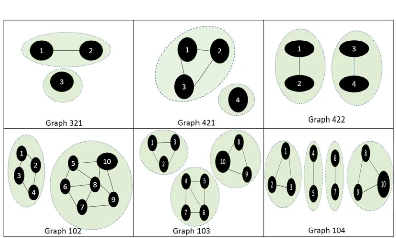
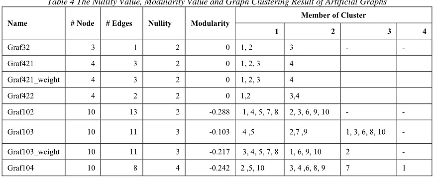
The first scenario was conducted by calculating the nullity value of each graph in the list of artificial graphs and viewing the Laplacian matrix form of each graph. Table 4 shows the experiment results, that are the computed nullity value on the Nullity column, the cluster formed in Member of Cluster column along with the detail cluster members from each graph, and the modularity value. We compare the result on Table 4 to the block diagonal matrix form represented on Figure 7.

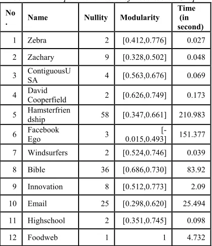
The second scenario was designed to investigate whether nullity values can lead to normal cluster quality, by looking at the modularity value. The second scenario experiment was applied to each real-world graph, and each graph was tested ten times. In each test, it was recorded the modularity value to know the range of modularity values obtained in the tests. This procedure was conducted as considering the randomly initial center at the time of running the K-Means algorithm. By experimenting several times, it was expected that the data obtained can provide a complete picture. While the process time listed was the average processing time of ten experiments. Table 5 summarizes the experimental results data.

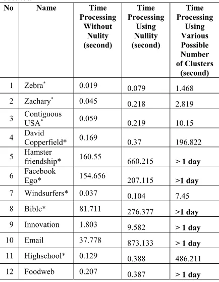
The third scenario was to find out the additional time required by adding the process of calculating the value of nullity; those are step 2 and step 3 on the algorithm listed in Modified Graph Spectral Algorithm. To conceive the condition, it was run original spectral graph clustering and modified

spectral graph clustering algorithm for each graph using the same cluster number values and compared the required processing time. The time processing data is presented in Table 6.

5. DISCUSSION 5.1 The Artificial Graphs

The experiment result using the artificial graph as appearing on the data in Table 4 shows that the calculated nullity value is indeed equal to the number of clusters in a graph. Likewise, with the value of modularity obtained for Graf32, Graf421, Graf421_weight and Graf422. The value of the modularity of the cluster results of the four graphs is zero, indicating the number of clusters and members of each cluster accordingly. Meanwhile, though the calculated nullity value for Graf102, Graf103, Graf103_weight, and Graf104 is equal to the real number cluster in the graph, the modularity value is negative since the members of the individual do not match the specified conditions. This phenomenon can occur because of the nature of the K-Means algorithm that has a weakness called trapped at the local optimum, where the algorithm is already convergent but has not provided an appropriate result. Nevertheless, this result not cancelling the proof of the ability of nullity to predict the number of clusters in the graph. So, it can be sure that the nullity value can be used as a tool to predict the best amounts of clusters contained in a graph.

This conclusion was also supported by the matrix shown in Figure 7, that shows the block diagonal matrix form of the Laplacian matrix of the adjacency matrix of the graphs.

Table 4 The Nullity Value, Modularity Value and Graph Clustering Result of Artificial Graphs

Name # Node # Edges Nullity Modularity Member of Cluster

1 2 3 4

Graf32 3 1 2 0 1, 2 3 - -

Graf421 4 3 2 0 1, 2, 3 4

Graf421_weight 4 3 2 0 1, 2, 3 4

Graf422 4 2 2 0 1,2 3,4

Graf102 10 13 2 -0.288 1, 4, 5, 7, 8 2, 3, 6, 9, 10 - -

Graf103 10 11 3 -0.103 4 ,5 2,7 ,9 1, 3, 6, 8, 10 -

Graf103_weight 10 11 3 -0.217 3, 4, 5, 7, 8 1, 6, 9, 10 2 -

2048 Notice the size of each Laplacian Matrix of the adjacency matrix of each artificial graph is equal to the number of vertices in the graph. The row index in the matrix is related to the index of the vertices, and the block diagonal matrix is connected to the clusters in each graph. For example, consider the Laplacian matrix for Graph103 in Figure 7.

Table 5 The Experiment Result of Real-World Graph

No

. Name Nullity Modularity

Time (in second)

1 Zebra 2 [0.412,0.776] 0.027

2 Zachary 9 [0.328,0.502] 0.048

3 ContiguousU_SA 4 [0.563,0.676] 0.069

4 David _Cooperfield 2 [0.626,0.749] 0.173

5 Hamsterfrien_dship 58 [0.347,0.661] 210.983

6 Facebook _Ego 3 _0.015,0.493] [- 151.377

7 Windsurfers 2 [0.524,0.746] 0.039

8 Bible 36 [0.686,0.730] 83.92

9 Innovation 8 [0.512,0.773] 2.09

10 Email 25 [0.298,0.620] 25.494

11 Highschool 2 [0.351,0.745] 0.098

12 Foodweb 1 1 4.732

There are three block matrices arranged diagonally, where the first block relates to the first cluster in Graph103 in Figure 6, where first cluster members are nodes 1,2 and 3, the second cluster consisting of nodes 4,5,6 and 7, and the third cluster consists of nodes 8,9 and 10. This result also assure us that the nullity of the Laplacian matrix of the adjacency matrix can be used as a tool to predict the number of the clusters in the graph.

Experiment result of the artificial graph also shows that the nullity value can be used to predict the number of clusters for unweighted and weighted graphs. This can be seen from the nullity value of Laplacian Matrix of Graph421_weight and Graph103_weight is equal to the number of clusters defined, also we find the block diagonal matrix form for both graphs is symmetric, and the eigenvalue for each block is zero.

2049

Table 6 Time Processing Comparison using Each Method

No Name Time

Processing Without

Nulity (second)

Time Processing

Using Nullity (second)

Time Processing

Using Various Possible Number of Clusters (second) 1 Zebra* _0.019

0.079 1.468 2 Zachary* _0.045

0.218 2.819

3 Contiguous _USA* 0.059 _{0.219 10.15}

4 David _Copperfield* 0.169 _{0.37 196.822}

5 Hamster _friendship* 160.55 _{660.215 > 1 day}

6 Facebook _Ego* 154.656 _{207.115 >1 day}

7 Windsurfers* 0.037 _{0.104 7.45}

8 Bible* 81.711 _{276.377 >1 day}

9 Innovation 1.803 _{9.582 > 1 day}

10 Email 37.778 _{873.133 > 1 day}

11 Highschool* 0.129 _{0.388 486.211}

12 Foodweb 0.207 _{0.387 > 1 day}

5.2 The Real-World Graphs

Furthermore, to examine the performance of proposed technique in predict the number of clusters in various types and graph size we conduct the experiment using the Real-World graph. Measurements were made adopting indirect method by looking at the modularity value of clustering result. This is done because there is no the ground truth number of clusters of each cluster. It is expected that by using calculating the nullity value technique will be obtained a modularity value greater than zero.

The modularity value shown in the Table 5 for almost graph is in the range 0.3-0.8 point except for Foodweb graph. According to Girvan Newman this is the normal range modularity value for the real-world graph, where actually the best modularity value for real world graph is between 0.3-0.7[15]. The nullity value of Foodweb graph is 1, means the graph has a sturdy structure or each node has a strong relation with the other node so we cannot find smaller subgraph in the original graph. So that, in general the experiment shows for various sizes graph, starting from the graph consisting of dozens of vertices and edges up to that have thousands of vertices and edges can reach the normal range of

modularity when it is processed by the proposed algorithm. It is concluded that using the nullity as a means of predicting the number of clusters can support the achievement of the best possible number of clusters and resulting in the qualified cluster.

The experimental results using real-world data also showed that predicting the number of clusters contained in a graph using the nullity value of the Laplacian matrix of the adjacent matrix of a graph can also be applied to an undirected or directed graph. The Innovation, Email, Highschool, and Foodweb graphs are examples of the directed graphs. The modularity values of those graphs also in the range of accepted value for the real-world graph. The condition happens because it is possible to change a directed graph into an undirected graph, considering there is no critical information is reduced. As for the directed graph, in this experiment, it was performed the preprocesses by forming directed graphs into non-directional graphs, because after we analyze the data we found no essential information is ignored by turning directed graphs into undirected one. For the case of unweighted directed graphs, it was defined the edge weight is one, while for directed-weighted graphs are transformed into undirect-weighted graphs by summing the weights of each directed edge. Based on these facts it can be deduced for various sizes and types of graphs, we can predict the number of the cluster in a graph using the nullity of Laplacian Matrix of the adjacency matrix of the graph.

2050 obtained have a firm basis compared with trial and error.

Later, it was compared the values in the fourth column and fifth column. The fifth column in Table 6 showed the time processing when the method of trying all possible number of clusters was used to determine the number of clusters that result in the highest modularity value. By comparing the values in the fourth column and the fifth column, it is clear the performance of modified algorithms is much better. The method of comparing the various number of clusters may be the same as repeating the clustering process using the original algorithm as much as the number of vertices in the graph. Of course, it takes a very long time. Thus, by comparing the additional time required to compute the nullity and the time process examining all possible cluster numbers, evidently, the computation of nullity values is more efficient. Based on these comparisons, it can be concluded that the time performance of the modified graph clustering is more efficient.

Also, to note, the method of comparing the number of clusters aiming to obtain the best number of clusters is not appropriate. Especially for graph spectral clustering algorithm that involving the k-means algorithm in it. It is noticed, the weakness of k-means algorithm is the trapped on the local optimum. The condition means the iteration will be breaking because the process considered convergent, though the solution obtained has not been the most optimal solution. Thus, there is a condition at the same number of clusters, the value of modularity obtained varies. The phenomenon is influenced by the initial center point chosen at the beginning of the iteration. If the initial center selected at the beginning of the iteration is close to the optimum global solution, then cluster process may result in an optimal solution. Conversely, if the chosen initial center point is far from the optimum global solution, and even closer to the point that resulted in the trapped on local optimum condition, then the solution obtained is not the best solution. The modularity value in Table 4 also shows this phenomenon. It is noticed, the modularity value data was obtained from ten times experiment using the same number of clusters but a set of different initial center points, that is chosen randomly. Different initial center points resulting various modularity value. Therefore, to obtain a legitimate optimal value, for every possible number of clusters, then the ideal way to run the method is to try all possible combinations of the initial center point. For

example, if on a graph there are ten nodes, namely 1, 2, 3, ..., 10 then the number of possible clusters is 2,3, 4, ..., 10. When the number of groups is 2, it should be tested all combinations of 2 nodes as the initial center point from the existing 10 nodes, which is about 45 combinations, to conclude the best maximum modularity value at the number of clusters is two. When the number of clusters is three, it should be examined all the combinations of 3 nodes from 10 nodes, which is about 120 combinations, then taken the maximum modularity value. The procedure should be repeated for all possible number of the clusters. After that, the maximum modularity value of each number of clusters is compared once more to find the greatest modularity value. This condition is inefficient, especially if the number of vertices and sides is very much. Thus, in the future it is necessary to find a method to choose the best initial center point to complete the nullity method as a tool to predict the best cluster number in graph clustering.

To sum up, by conducting experiments using artificial data or real data it is proven using the nullity value as a tool to predict the number of clusters contained in a graph can be done more efficiently than by doing repeatedly approach or by experimenting with various possible number of clusters. By using the nullity value technique, the calculation is done only once because the calculation of the nullity value of the Laplacian matrix is a structured method and clear stages. Also, the technique can be used to process any type and size of data that is showed from the performance measurement.

6. CONCLUSION

The nullity of the Laplacian Matrix of the adjacency matrix of the Graph is a simple and more efficient method to predict the number of clusters in Graph Clustering than trial and error method. The approach can be implemented for various size of graphs that have a dozen vertices up to thousands of nodes and edges, also can be applied to different types of graph, such as an undirected-unweighted graph, unweighted graph, directed-weighted graph and directed-directed-weighted graph.

2051

REFERENCE

[1] C. Dhanjal, R. Gaudel, and S. Clémençon, “Efficient eigen-updating for spectral graph clustering,” Neurocomputing, vol. 131, pp. 440–452, 2014.

[2] B. Hendrickson and R. Leland, “An improved spectral graph partitioning algorithm for mapping parallel computations,” SIAM J. Sci.

Comput., vol. 16, no. 2, pp. 452–469, 1995.

[3] M. Fiedler, “Laplacian of graphs and algebraic connectivity,” Banach Cent. Publ., vol. 25, no. 1, pp. 57–70, 1989.

[4] T. Bühler and M. Hein, “Spectral clustering based on the graph p-Laplacian,” in Proceedings of the 26th Annual International

Conference on Machine Learning, 2009, pp.

81–88.

[5] I. S. Dhillon, Y. Guan, and B. Kulis, A unified view of kernel k-means, spectral clustering

and graph cuts. Citeseer, 2004.

[6] I. Atastina, B. Sitohang, G. A. S. Putri, and V. S. Moertini, “Graph clustering using dirichlet process mixture model,” in Data and Software Engineering (ICoDSE), 2017

International Conference on, 2017, pp. 1–5.

[7] C. Fraley and A. E. Raftery, “How many clusters? Which clustering method? Answers via model-based cluster analysis,” Comput. J., vol. 41, no. 8, pp. 578–588, 1998.

[8] S. Salvador and P. Chan, “Determining the number of clusters/segments in hierarchical clustering/segmentation algorithms,” in Tools with Artificial Intelligence, 2004. ICTAI 2004.

16th IEEE International Conference on,

2004, pp. 576–584.

[9] X. Hu and L. Xu, “Investigation on several model selection criteria for determining the number of cluster,” Neural Inf. Process.-Lett. Rev., vol. 4, no. 1, pp. 1–10, 2004.

[10] R. Tibshirani, G. Walther, and T. Hastie, “Estimating the number of clusters in a data set via the gap statistic,” J. R. Stat. Soc. Ser. B

Stat. Methodol., vol. 63, no. 2, pp. 411–423,

2001.

[11] A. Fujita, D. Y. Takahashi, and A. G. Patriota, “A non-parametric method to estimate the number of clusters,” Comput. Stat. Data

Anal., vol. 73, pp. 27–39, 2014.

[12] E. Y. Baagyere, Z. Qin, H. Xiong, and Q. Zhiguang, “The Structural Properties of Online Social Networks and their Application Areas.,” IAENG Int. J. Comput. Sci., vol. 43, no. 2, 2016.

[13] D. A. Bader, H. Meyerhenke, P. Sanders, C. Schulz, A. Kappes, and D. Wagner,

“Benchmarking for graph clustering and partitioning,” in Encyclopedia of Social

Network Analysis and Mining, Springer,

2014, pp. 73–82.

[14] M. C. Nascimento and A. C. De Carvalho, “Spectral methods for graph clustering–a survey,” Eur. J. Oper. Res., vol. 211, no. 2, pp. 221–231, 2011.

[15] M. E. Newman and M. Girvan, “Finding and evaluating community structure in networks,”