Content based Trademarks Retrieval using Bag of Visual Words
M. Ramesh Kumari
Lecturer (Senior Grade)
Department of Computer Science & Engineering
Ayyanadar Janaki Ammal Polyechnic College, Sivakasi, India
Abstract— Trademarks are distinctive visual symbols used to identify and distinguish a specific product, service or business. With the rapid increase in the amount of registered trademark images around the world, Trademark Image Retrieval (TIR) has emerged to ensure that new trademarks do not repeat any of the vast number of trademark images stored in the trademark registration system. Content Based Image Retrieval (CBIR) method is a promising method for performing trade mark retrieval. In this work, Histogram of Oriented radiant (Hog) algorithm is developed to draw the histogram for the gradient image for the given trade mark logo. Addition, an L1 Distance algorithm is developed to find similarity between query image and database images by comparing the corresponding histograms and to obtain images similar to query image from data base. Precision and recall method is used to evaluate the performance of above mentioned algorithms and results obtained are compared with the results of SIFT algorithm obtained from literature. It is found that the HOG algorithm is better with 96% of retrieval efficiency than SIFT algorithm which has retrieval efficiency of 94% only.
Key words: Multimedia Object, Text Detection, Localization, Tracking, Extraction, Enhancement
I. INTRODUCTION
A. What is CBIR?
The earliest use of the term content-based image retrieval in the literature seems to have been by Kato [1992], to describe his experiments into automatic retrieval of images from a database by color and shape feature. The term has since been widely used to describe the process of retrieving desired images from a large collection on the basis of features (such as colour, texture and shape) that can be automatically extracted from the images themselves. The features used for retrieval can be either primitive or semantic, but the extraction process must be predominantly automatic. Retrieval of images by manually-assigned keywords is definitely not CBIR as the term is generally understood – even if the keywords describe image content.
CBIR differs from classical information retrieval in that image databases are essentially unstructured, since digitized images consist purely of arrays of pixel intensities, with no inherent meaning. One of the key issues with any kind of image processing is the need to extract useful information from the raw data (such as recognizing the presence of particular shapes or textures) before any kind of reasoning about the image’s contents is possible. Image databases thus differ fundamentally from text databases, where the raw material (words stored as ASCII character strings) has already been logically structured by the author [Santini and Jain, 1997]. There is no equivalent of level 1 retrieval in a text database.
CBIR draws many of its methods from the field of image processing and computer vision, and is regarded by some as a subset of that field. It differs from these fields principally through its emphasis on the retrieval of images with desired characteristics from a collection of significant size. Image processing covers a much wider field, including image enhancement, compression, transmission, and interpretation. While there are grey areas (such as object recognition by feature analysis), the distinction between mainstream image analysis and CBIR is usually fairly clear-cut. An example may make this clear. Many police forces now use automatic face recognition systems. Such systems may be used in one of two ways. Firstly, the image in front of the camera may be compared with a single individual’s database record to verify his or her identity. In this case, only two images are matched, a process few observers would call CBIR. Secondly, the entire database may be searched to find the most closely matching images. This is a genuine example of CBIR
B. Image Representation with a Bag of Visual Words
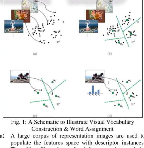
[image:1.595.307.548.450.697.2]The Bag-of-visual –words is an analogy to the computer vision domain of the classic bag-of-words. The common text description of a “bag-of-words” can be mapped over to the visual domain: the image’s empirical distribution of words is captured with a histogram counting how many times each word in the visual vocabulary occurs within it.
Fig. 1: A Schematic to Illustrate Visual Vocabulary Construction & Word Assignment
a) A large corpus of representation images are used to populate the features space with descriptor instances. The white ellipse denote local feature regions and the black dots denote points in some feature space eg., SIFT. b) Sampled features are clustered in order to quantize the
space into a discrete number of visual words.
d) A bag-of-visual words histogram can be used to summarize the entire image. It counts how many times each of the visual words occurs in the image.
C. Application of Content based Trademarks Retrieval
With the rapid increase in the amount of registered trademark images around the world, trademark image retrieval (TIR) has emerged to ensure that new trademarks do not repeat any of the vast number of trademark images stored in the trademark registration system. As the traditional classification of trademark images is based on their shape features and types of object depicted by employing manually assigned codes, faults or slips may appear because of different subjective perception of the trademark images. Evidence has been provided that the traditional classification is not feasible in dealing with a large fraction of trademark images with little or no representational meanings.
Trademarks can be categorized into a few different types. A trade- mark can be a word-only mark, a device-only mark or a device- and-word mark. For a word-only mark, the design of the trademark consists purely of text words or phrases. However, for a device only mark, the trademark only contains symbols, icons or images. If a trademark comprises both words and any iconic symbols or images, it can be regarded as a device and word mark. Since different algorithms have to be used in describing different kinds of trademark images, a trademark image retrieval system can only be designed to accommodate one of the types. Although several trade- mark image retrieval systems have been designed to handle all kinds of trademark images, the performance of these systems are rather unfavorable. When compared to those systems that are specifically designed to handle only one kind of trademark. Another challenge in trademark image retrieval is the difficulty in modeling human perception about similarity between trademarks. As human perception of an image involves collaboration between different sensoria, it is in fact difficult to integrate such human perception mechanisms into a trademark image retrieval system. This project work aims at developing a robust method for trademark image retrieval to cope with rotation, scale and illumination changes. Given a query logo image, our goal is to retrieve all logo images similar to the query logo in a database of trademark images.
D. Advantages of Content based Trademarks Retrieval
The trademarks recognition is affected mostly by scaling, illumination, rotation in the feature extraction process. Processing time for recognition is more. To identify trademarks using their shape, color, and texture features are very important. If any paper considers all three features (shape, color, texture) then the accuracy is very less. To overcome the Illumination, scaling and rotation-invariant problems in trademarks recognition with improved efficiency. To recognize trademarks using their features extracted from images by HOG.
[image:2.595.310.530.69.260.2]E. Over All Module Design
Fig. 2: Module Design
II. OBJECT & FEATURE EXTRACTION
A. Basic Global Thresholding Algorithm
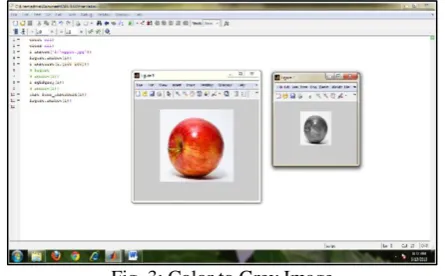
In this project Basic global thresh-holding algorithm is used to compute an optimal threshold for separating the data into two classes. As a first step the given color image is converted into grey image as shown in fig 3.1. Then histogram is initially segmented into two parts using a randomly select starting threshold value T(1).The data are classified into two classes (c1 and c2).Then, a new threshold value is computed as the average of the above two sample means. This process is repeated until the threshold value does not change any more. Segmentation involves separating an image into regions (or their contours) corresponding to objects. We usually try to segment regions by identifying common properties. Or, similarly, we identify contours by identifying differences between regions (edges). The simplest property that pixels in a region can share is intensity. So, a natural way to segment such regions is through thresholding, the separation of light and dark regions. Thresholding creates binary images from grey level ones by turning all pixels below some threshold to zero and all pixels about that threshold to one.
If g(x, y) is a threshold version of f(x, y) at some global threshold T,
g(x, y) = 1 if f(x, y) ≥ T 0 otherwise
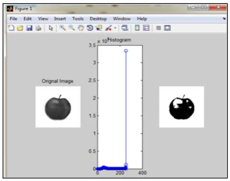
[image:2.595.317.540.625.763.2]Fig. 4: Basic Thresh-Hold Output
B. Edge Detection Algorithm
The purpose of edge detection in general is to significantly reduce the amount of data in an image, while preserving the structural properties to be used for further image processing. Several algorithms exists, and this work focuses on a particular one developed by John F. Canny (JFC). Even though it is quite old, it has become one of the standard edge detection methods and it is still used in research.
1) The Canny Edge Detection Algorithm
The algorithm runs in 3 separate steps:
1) Smoothing: Blurring of the image to remove noise. 2) Finding gradients: The edges should be marked where
the gradients of the image has large magnitudes. 3) Non-maximum suppression: Only local maxima should
be marked as edges. a) Smoothing
It is inevitable that all images taken from a camera will contain some amount of noise. To prevent that noise is mistaken for edges, noise must be reduced. Therefore the image is first smoothed by applying a Gaussian filter. The kernels of a Gaussian filter with a standard deviation.
b) Finding Gradients
The Canny algorithm basically finds edges where the gray scale intensity of the image changes the most. These areas are found by determining gradients of the image. Gradients at each pixel in the smoothed image are determined by applying what is known as the Sobel-operator. First step is to approximate the gradient in the x- and y-direction respectively by applying the kernels shown in Equation (2).
The gradient magnitudes (also known as the edge strengths) can then be determined as a Euclidean distance measure by applying the law of Pythagoras as shown in Equation (3). It is sometimes simplified by applying Manhattan distance measure as shown in Equation (4) to reduce the computational complexity. The Euclidean distance measure has been applied to the test image.
c) Non-Maximum Suppression
The purpose of this step is to convert the “blurred” edges in the image of the gradient magnitudes to “sharp” edges. Basically this is done by preserving all local maxima in the gradient image, and deleting everything else. The algorithm is for each pixel in the gradient image:
1) Round the gradient direction to nearest 30◦, corresponding to the use of a 12-connected neighborhood.
2) Compare the edge strength of the current pixel with the edge strength of the pixel in the positive and negative gradient direction. I.e. if the gradient direction is north (theta = 90◦), compare with the pixels to the north and south.
3) If the edge strength of the current pixel is largest; preserve the value of the edge strength. If not, suppress (i.e. remove) the value.
[image:3.595.311.541.275.452.2]A simple example of non-maximum suppression is shown in Figure 3.3 Almost all pixels have gradient directions pointing north. They are therefore compared with the pixels above and below. The pixels that turn out to be maximal in this comparison are marked with white borders. All other pixels will be suppressed. Figure 3.3 shows the effect on the test image.
Fig. 5: Original & Smoothed
Fig. 6: Gradient Magnitudes & Final Output
III. DEVELOPMENT OF HOG & L1 DISTANCE ALGORITHMS
A. Histogram of Oriented Gradients (HOG)
The essential thought behind the Histogram of Oriented Gradient descriptors is that local object appearance and shape within an image can be described by the distribution of intensity gradients or edge directions. The implementation of these descriptors can be achieved by dividing the image into small connected regions, called cells, and for each cell compiling a histogram of gradient directions or edge orientations for the pixels within the cell. The combination of these histograms then represents the descriptor. For improved accuracy, the local histograms can be contrast-normalized by calculating a measure of the intensity across a larger region of the image, called a block, and then using this value to normalize all cells within the block. This normalization results in better invariance to changes in illumination or shadowing.
B. Orientation Binning
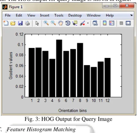
The next step is to compute cell histograms for later use at descriptor blocks. Computed with 12 orientation bins for [0°, 360°] interval.
[image:4.595.50.287.147.373.2]For each pixel’s orientation, the corresponding orientation bin is found and the orientation is voted to this bin. The HOG output for query image is shown in figure.
Fig. 3: HOG Output for Query Image
C. Feature Histogram Matching
Histogram matching is a technique which is used to compare the histogram of two images. According to the histogram comparison value, the result is predicted. L1 Distance method is used for comparing histograms.
1) L1 Distance Method
It is also called the Manhattan Distance. If u=(x1, y1) and v=(x2, y2) are two points, then the Manhattan Distance between u and v is given by
MH(u,v)=|x1-x2|+|y1-y2| (5) Instead of two dimensions, if the points have n-dimensions. Such as a=(x1,x2,…..xn) and b=(y1,y2,……yn) then,eq.5 can be generalized by defining the Manhattan distance between a and b as
MH(a,b)=|x1-y1|+|x2-y2|+…..+|xn-yn|
Here we have used L1 Distance histogram comparison method.
IV. CODE DEVELOPMENT
This chapter discusses Basic global thresholding algorithm, Edge Detection Algorithm, Gradient computation, magnitude of the gray level gradient, Orientation Binning algorithm, and HOG Matching Algorithms l1 distance) which are developed using MATLAB.
A. Coding Description
HOG Computes Histogram of Oriented Gradient over a ROI. [BH, BV] = PHOG (I, BIN, ANGLE, L, ROI) computes phog descriptor over a ROI.
Given and image I, phog computes the Pyramid Histogram of Oriented Gradients over L pyramid levels and
1) Input
I - Images of size MxN (Color or Gray) bin - Number of bins on the histogram angle - 180 or 360
L - number of pyramid levels
roi - Region Of Interest (ytop, ybottom, xleft, xright)
B. Output
p - histogram of oriented gradients
C. Functions Used
The functions of MATLAB, which are used in this project are as follows,
Imread() Read the images
size(x) Returns the size of each dimension of array x
Imresize(a,scale) Returns the image that is scale the size of a
rgb2gray() Convert the true color image to gray color image
bar() Draw bar graph
xlswrite() Write to the xls file
gradient(F)
Gradient (F) where F is a vector returns the one-dimensional numerical gradient of F. FX corresponds to ∂F/∂x, the differences in x (horizontal)
direction.
zeros(n) returns an n-by-n matrix of zeros.
bwlabel() Label connected components in 2-D binary image
find() returns the indices of the array X that point to nonzero elements
xlsread(‘filename’)
returns numeric data in array , from the first sheet in Microsoft Excel
spreadsheet file named filename Table 1: Function of Mat Lab
V. RESULT & DISCUSSION
A. Introduction
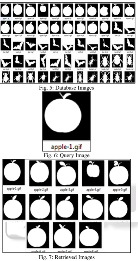
Fig. 5: Database Images
Fig. 6: Query Image
Fig. 7: Retrieved Images
B. Performance Evaluation of the Proposed System
The precision and recall method is used to evaluate the performance of the proposed system and the same precision and recall method is used to evaluate the SIFT system. The formulas used are given below
Precision = No. of relevant images retrieved / Total no. of images retrieved
Recall = No. of relevant images retrieved / Total no. of relevant images in the database
The retrieval efficiency (RE) is given by:
R.E = No. of relevant images retrieved / Total no. of images retrieved N <=R
No. of relevant images retrieved / Total no. of relevant images otherwise
Where, N = no. of retrieved images R = no. of relevant images
The results of retrieval efficiency of SIFT and HOG methods are shown in table 6.1 and 6.2 respectively. The tables show that HOG method is better with 96% retrieval efficiency than SIFT which has a retrieval efficiency of 94%.
Retrievals 10 20 40 50 Precision 1 1 0.95 0.94
Recall 0.2 0.4 0.76 0.94 Error Rate 0 0 0.052 0.063
Retrievals Efficiency
[image:5.595.321.539.64.223.2]100 100 95 94 Table 2: Retrieval Efficiency for SIFT Retrievals 10 20 40 50
Precision 1 1 0.975 0.96 Recall 0.2 0.4 0.78 0.96 Error Rate 0 0 0.025 0.041
Retrievals Efficiency
100 100 97.5 96 Table 3: Retrieval Efficiency for Proposed Method
VI. CONCLUSION
The proposed system using Basic global thresholding algorithm, Edge Detection Algorithm, Gradient computation, magnitude of the gray level gradient, Orientation Binning algorithm, and HOG MATCHING Algorithms l1 distance).
Object is extracting by using Basic global thresholding algorithm. The extracted image is converted into gradient image using gradient computation and Magnitude of gray level gradient algorithm. Using orientation binning algorithm the gradient image is segmented into 12 orientation bins for [0°,360°] interval and drawn a histogram.
L1 Distance Algorithm is developed to find similarity between query image and database images by comparing the corresponding histograms and to obtain images similar to query image from data base. Precision and recall method is used to evaluate the performance of above mentioned algorithms and results obtained are compared with the results of SIFT algorithm obtained from literature. It is found that the HOG algorithm is better with 96% of retrieval efficiency than SIFT algorithm which has retrieval efficiency of 94% only.
REFERENCES
[1] Ahmed Zeggari, Fella Hachouf, SebtiFoufou, “Trademarks recognition Based on Local Regions Similarities” 10th international conference on information science,signal processing and their applications(ISSPA 2010).
[2] HichemSahbi, LambertoBallan, Giuseppe Serra, and Alberto Del Bimbo, “Context-Dependent Logo Matching and Recognition”, IEEE Transaction on image processing ,2013
[3] ManimalaSingha and K.Hemachandran,” content Based Image Retrieval using Color and Texture”, an international journal (SIPIJ) vol.3 no.1 Feb 2012. [4] Rafael C. Gonzalez, Richard E. Woods, Steven
L.Eddins, Digital Image Processing Using MatLab MC Graw Hill
[5] Y.M.Latha ,Jinaga. B.C and Reddy. V.S.K, “Content Based Color Image Retrieal via Wavelet Transforms”, IJCSNS international Journal of computer science and network security ,Vol 7 no.12,Dec 2007