Boundary Value Problems for Burgers Equations, through Nonstandard Analysis

(1)

http://dx.doi.org/10.4236/am.2015.66099

Boundary Value Problems for Burgers

Equations, through Nonstandard Analysis

Saida Bendaas

Department of Mathematics, Faculty of Sciences, University of Setif 1, Elbez, Algeria Email: [email protected]

Received 22 April 2015; accepted 7 June 2015; published 10 June 2015

This work is licensed under the Creative Commons Attribution International License (CC BY). http://creativecommons.org/licenses/by/4.0/

Abstract

In this paper we study inviscid and viscid Burgers equations with initial conditions in the half plane x∈R T, >0. First we consider the Burgers equations with initial conditions admitting two

and three shocks and use the HOPF-COLE transformation to linearize the problems and explicitly solve them. Next we study the Burgers equation and solve the initial value problem for it. We study the asymptotic behavior of solutions and we show that the exact solution of boundary value prob-lem for viscid Burgers equation as viscosity parameter is sufficiently small approach the shock type solution of boundary value problem for inviscid Burgers equation. We discuss both conflu-ence and interacting shocks. In this article a new approach has been developed to find the exact solutions. The results are formulated in classical mathematics and proved with infinitesimal tech-nique of non standard analysis.

Keywords

Non Standard Analysis, Boundary Value Problem, Viscid Burgers Equation, Inviscid Burgers Equation, Heat Equation

1. Introduction

The nonlinear parabolic partial differential equation

t x xx

u +uu =εu (1.1)

(2)

When ε is null, this equation approaches to the Euler’s equations in one dimension who governs the flows of perfect fluids. It’s the viscid equation. it has the form

0.

t x

u +uu = (1.2)

If the viscous term is dropped from the Burgers equation, discontinuities may appear in finite time; even if the initial condition is smooth, they give rise to the phenomenon of shock waves with important application in physics [3]. This property makes Burgers equation a proper model for testing numerical algorithms in flows where severe gradients or shocks are anticipated [4]-[6]. Discretization methods are well-known techniques for solving Burgers equation. Ascher and McLachlan established many methods as multi-symplectic box sheme. For the boundary value problem, Sinai [7] was interested to the initial condition case: null on R− and Brow-nian on R+. She, Aurell and Frich [8] with numerical calculations particularly examined the initial conditions of Brownian fraction nair to the asymptotic behavior.

A remarkable feature of viscid Burgers equation is that its solutions with initial conditions of the form

( )

, 0

( )

u ξ = f ξ (1.3) can be explicitly written down. Hopf [9] and Cole [10] independently showed that the Equation (1.1) can be li-nearized through the transformation

2 x .

u= − εϕ ϕ (1.4)

Then Hopf [9] showed that if φ

( )

x t, satisfies the linear heat equation

t xx

ϕ =εϕ (1.5)

with initial condition

( )

1 ₀

( )

(

)

2

, 0 exp d d .

2 2

x

x f

t η

ϕ ν ν η

ε ∞

  ₋ 

 

= −  + 

 _ _



∫



(1.6)

Then u x t

( )

, defined by Equation (1.4) solves (1.1) and (1.3). Conversely, if u x t

( )

, is a solution of prob-lem (1.1) and (1.3) then ϕ

( )

x t, defined by Equation (1.4) is a solution of problem (1.5) and (1.6). Solving for

ϕ from (1.5) and (1.6) and substituting it into Equation (1.3) we obtained explicit formula for the solution of problem (1.1) and (1.2) namely:

( )

(

)

( )

(

)

2

0

2 1

exp d d

2 2

,

1

exp d d

2 2

x x

f

t t

u x t

x f

t η

η _{ν ν} _η

ε

η

ν ν η

ε

∞ ∞

−∞

∞ −∞

  ₋ 

− _₋ _ ₊ __

 _ _

 

=

  ₋ 

−  + 

 _ _

 

∫

(1.7)

and studied the asymptotic behavior of u x t

( )

, .

Explicit solutions of the Burgers equation (1.1) in the quarter plane with integrable initial data and piecewise constant boundary data were constructed by [11] using Hopf-Cole transformation [9]. He obtained a formula for its weak limit as viscosity parameter goes to 0. Although, there are many results for initial value problem has been studied less. Using maximum principle, this formula for weak limit was extended to general boundary data.

ε is a positive parameter small enough. The problem is considered by [12]. As the fact that ε multiplies the larg-est derivative, one is in the presence of a singular perturbation problem. The purpose of Singular Perturbation Theory is to investigate the behavior of solutions of (1.1) as ε→0.

The aim of the present article is to study solutions of Inviscid and Viscid Burgers equation if the initial condi-tion admits several singular points, i.e. in the case of a finite number of shocks. A simple formulation is given for the asymptotic behavior based on the evaluation of integrals which is a method of the non standard perturba-tion theory of differential equaperturba-tions proposed by Imm Van Den Berg [13] and improved by Lutz and Callot.

(3)

into the field of perturbed differential equations. Our goal in this paper is to generalize these techniques on EDP and our general purpose is to describe the asymptotic behavior of solutions in boundary value problem with a small parameter ε and to discuss in particular the cases of confluence and the interacting shocks with new tech-nical infinitesimal of non-standard analysis. We can conclude that the solutions of the problem: (1.1) and (1.3) are infinitely close to the solutions of problems (1.2) and (1.3), as ε is a parameter positive sufficiently small.

In Section 2, we treat the boundary value problem for inviscid Burgers equation, solve it and study it. Section 3 is devoted to useful lemmas for our main results. In Section 4, we study viscid Burgers equation, solve exactly the initial value problems for it, and describe the asymptotic behavior of solutions with a non standard form. Some components, such as multi-leveled equations, graphics, and tables are not prescribed, although the various table text styles are provided. The formatter will need to create these components, incorporating the applicable criteria that follow.

2. Initial Boundary Value Problem for Inviscid Burgers’ Equation

2.1. Shock Fitting

We consider the inviscid Burgers equation:

0.

t x

u +uu =

In: x∈R, t>0 with the initial condition

( )

, 0

( )

u ξ = f ξ

where f R: →R, is continuous.

This problem not admits the regular solutions but some weak solutions with certain regularity exist. The Burgers equation on the whole line is known to possess traveling wave solutions. The solution of (1.2) and (1.3) may be given in a parametric form and shocks must be fitted in such that:

(

1 2

)

(

( )

1

( )

2

)

1 1

2 2

U= u +u = f ξ + f ξ (2.1) where ξ₁ and ξ₂ are the value of

ξ

on the two sides of the shock [16].

According to Equation (1.2), the solution at time t is obtained from the initial profile u= f

( )

ξ by translat-ing each point a distance f

( )

ξ t to the right. The shock cuts out the part corresponding to ξ₂≥ ≥ξ ξ₁. If the discontinuity line, it is a straight line chord property still holds. The cord on the f curve cuts off lobes of equal area. The shock determination can then be describe entirely on the fixe f

( )

ξ curve by drawing all the chords with the equal area property can be written analytically as between the points ξ ξ= ₁ and ξ ξ= ₂on the curve

( )

f ξ . Moreover since areas are preserved under the mapping, the equal area

( )

(

)

(

)

2

( )

1

1 2 1 2

1

d .

2 f f f

ξ ξ

ξ + ξ ξ ξ− =

_∫

ξ ξ (2.2)

This is the differential equation for the line cord of shock that checks the condition of entropy such as [16] [17]

Corresponding to the two inflection points.

2.2. Confluence of Shocks

When a number of shocks are produced, in general it is possible for one of them to overtake the shock ahead. Then they combine and continue as a single shock. This is also described by our shock solution.

Consider the curve given by fFigure 1, then two shocks are formed corresponding to the inflection points p

and q with families of equal area chords, typified by p p₁ ₂ and q q_{1 2}.

As time goes, the points q₁ and p₂ approach each other until the stage inFigure 2 is reached where a common chord cuts off lobes of equal area for both humps.

At this stage the characteristics corresponding to p₂′ and q₁′ are the same and therefore the shocks have just combined into one as shown in Figure 3. Characteristics p₂′ and q₁′ combined. All the characteristics be-tween q₂′ and p₁′ have now been absorbed by one or other of the shocks. A single shock proceeds using chords p q_{1 2}′′ ′′.

(4)

[image:4.595.128.494.70.718.2] [image:4.595.140.488.86.290.2]

Figure 1.Graphic representation of the initial condition f.

Figure 2. Graphical representation from the merger of the two shocks. The characteristics p₂′

[image:4.595.144.487.516.707.2]

and q1′ merge.

(5)

[image:5.595.145.479.93.297.2]

Figure 4. The (x, t) diagram for merging shocks corresponding toFigure 1.

3. Preliminaries

In this section we present some lemmas that are important to prove our main result.

Proposition 3.1.Let ϕ ϕ ϕ= ₁+ ₂ be the analytic solution for the initial value problem for the heat equation

(1.5) and (1.6). If the initial condition is given as in Figure 1, then u given by the Formula (1.4) is a solution for the initial value problem (1.1) and (1.3). It is explicitly given by:

1 1 2 2

1 2

2 x u u

u εφ ϕ ϕ

φ ϕ ϕ

+

= − =

+ (3.1)

i.e.

( )

(

)

( )

(

)

2 2

1 0

2 2

1 0

1

exp d d

2 2

, .

1 1

exp d d

2 2

4π

i

i i i

i

i i

i

x x

f

t t

u x t

x f

t η

η

η _{ν ν} _η

ε

η

ν ν η

ε ε

∞ = = −∞

∞ =

= −∞

 ₋ 

− _− ₊ _

 

 

=

 ₋ 

− + 

 

 

∫

∑

(3.2)

Proof: When a shock overtakes another shock, they merge into a single shock of increased strength as de-scribed in inviscid solution

(

ε=0

)

, on the f curve inFigure 1; It is possible to give a simple solution of Burg-ers equation that describes this process for arbitrary ε. The solution for a single shock is given in [3] [4] and the corresponding expression for ϕ may be written in the form:

2

1 2; exp , 1, 2.

2 4

i i

u u

x t b i

ϕ ϕ ϕ ϕ

ε ε

 

= + =  + −  =

  (3.3)

In the expression of solution for a single shock given in [3] [4], the parameters b₁, b₂ witch locate the initial position of the shock are taken to be zero. The expressions ϕ ϕ₁ ₂ are clearly solutions of the heat equation

(

ϕt =εϕxx

)

with

2

exp , 1, 2.

2 4

i i i

u u x t i

ϕ

ε ε

 

=  +  =

  (3.4)

Corresponding to the initial conditions:

( )

0 0 ₀

1

exp d , 1, 2

2

x

i f i i i

ϕ φ η η η

ε

 

= = _− _ =

(6)

Then the solutions of the heat equation are given as:

( )

(

)

2

0

1 1

exp d d , 1, 2

2 2

4π

i i

x

f i

t t

η

ϕ

ν ν

η

ε

 ₋ 

 

= − + =

 



∫



(3.6)

( )

(

)

2

0 1

exp d d

2 2

i i

i

i i i

x x

u f

t t

η

ϕ

ν ν

η

ε

+∞

−∞

 ₋ 

− _ _

= − +

 



∫



∫

(3.7)

Using Equations (1.4) and (3.1) we obtain the expression (3.2).

And to prove our results, we use the non standard analysis techniques, for that we consider the following lemma.

Lemma 3.2. (The Van. Den. Berg lemma [14]): Let h be a standard function, defined and increasing on

[0,+∞[ such that h

( )

ν

=a

ν

r

(

1+

δ

)

where δfor v ≃ 0. h

( )

ν >m

( )

ν q. And let ϕ be an intern function de- fined on ]0,+∞[ such that :

ϕ ν

( )

=b

ν

s

(

1+

δ

)

for v ≈0, and such that ∀ d > 0, ∃ standard k and standard c such that: ϕ ν

( )

<kexp cosh

(

( )

ν

)

, for v>d. Then

( )

₁ ₁

0

1 Γ

1

exp d

2

1 2

s s

r r

s b

h _r

ra

ν

ϕ ν ν

ε

ε ∞

+ +

   

   

   

+

 

 

−

  _ _

= ⋅

 

  _ _

 

 

∫

(3.8)

where a, r are positive standard, m and q are the both positive δ is an infinitesimal. b and s are standard, 0

b≠ and s> −1.

To give estimation to the solution, given by (3.2), we state the following lemma:

Lemma 3.3. Let ε be a positive real small enough. And let ϕ and h be two standard functions such that: h, is a C2 class function verified the Lemma 3, and admits on the ξ point a unique absolute minimum h′

( )

ξ =0 and

( )

0

h′′ ξ > . ϕ ξ

( )

≠0. It is S-continuous on ξ and satisfies the conditions of the Lemma 3 in the both ways. Then

( )

(

)

4π

exp d 1

2 h

h

η ε

ϕ η η ϕ ξ δ

ε ξ

∞ −∞

−

 

= +

 

′′

 

∫

(3.9)

δ is an infinitesimal.

Proof: To prove this lemma, we use the “Van Den Berg” method, lemmas: (5.6), (5.7) [14]. It consists in the following steps

1) Search for the absolute minimum (maximum) of the function under the exponential sign and bring it out. 2) Bring back the minimum (maximum) to the zero.

3) Searching the galaxy as well as the main galaxy where the function in the exponential sign is appreciable. 4) Calculate the integral.

As consequence we have the following lemma.

Lemma 3.4. Let f the initial condition as Figure 1. Assume: (H1): f R: →R is C2(R).

(H2): There exist a, b, c, d and e in R, with a < b < c < d < e, such that

( )

]

[ ] [

] [ ] [

( )

[ ]

0, if , , , and if , , ,

0, if , and if ,

f x x a b c x c d e

f x x a b x d e

′′

 ≥ ∈ −∞ ∈ ∞

  _′′

≤ ∈ ∈



Then for x and t fixed, the functions defined as:

(

, ,

)

₀

( )

d

(

)

2, 1, 2 2

i i

x h x t f i

t

η η

η =

_∫

ν ν+ − = (3.10)

(7)

( )

, 1, 2

i i

x=η +tf η i= (3.11)

And the condition: hi

(

ξi, ,x t

) (

hi ξi , ,x t

)

,

− ₌ +

is equivalent to the shock conditions:

( ) ( )

(

)

(

)

( )

1

d , 1, 2 2

i

i i i i

f f ξ f i

ξ

ξ− + ξ+ ξ−−ξ+ =

∫

−+ ν ν = (3.12)

Proof: Let f the initial condition given as in Figure 1, two shocks are formed corresponding to the inflection points of f

( )

ξ . for some time we see appear an area of three values for the solution u x t

( )

, . At first the wave breaks on the feature for which: f_i′

( )

x <0 and f xi′

( )

is a maximum during the time t=tc. Inside the zone

of each shock and for a point

( )

x t, , there are three characteristics corresponding to two minimum framing a maximum. When a shock overtakes another, they merge into a single shock of increased strength as describe for the inviscid solution

(

ε=0

)

on the f curve in Figure 2. The characteristics between q₂′ and p₁′ are ab-sorbed by oneFigure 3. At this stage there are two stationary values that satisfy the equations (3.11) we noted them by ξ_i− and ξ_i+,i=1, 2, each couple frames a maximum. Let: η_i

( )

x t, , be the minimum for the functions given by the Formula (3.10), is such that:

( )

0, 1, 2

i i

h x

f i

t η η

η

∂ −

= − = =

∂

This equation is verified at the two minima ξ_i− and ξ_i+,i=1, 2. If hi

(

ξi , ,x t

) (

hi ξi , ,x t

)

,

− ₌ +

and within (3.10) this condition can be written as:

( )

(

)

( )

(

)

2 2

0 d ₂ 0 d ₂ , 1.2

i x i i x i

f f i

t t

ξ ξ ξ ξ

ν ν ν ν

+ − + − − −

+ = + =

∫

(3.13)

But ξ_i− and ξ_i+ both verify the equations:

( )

i 0, 1, 2

i

x

f i

t ξ

ξ −_ − _= =

  (3.14)

The condition of the shock is expressed by (3.12), is the same condition of shock given by (2.2) for invicid Burgers equation.

4. Initial Boundary Value Problem for Inviscid Burgers’ Equation

4.1. Confluence of Shocks

Our general purpose now is to show that the exact solution of (1.1) and (1.3) endorse the ideas regarding shocks in Section 2, we want to confirm that as ε is small enough, the solution of (1.1) and (1.3) reduce to solution of (1.2) and (1.3), with discontinuous shocks which satisfy the condition (2.2), and the shocks are located at the positions determined in Section 2. The shocks are formed corresponding to the inflection points of the initial condition u x

( )

, 0 = f x

( )

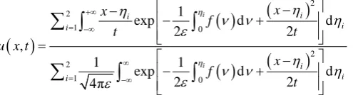
, who assume the assumptions (H1), (H2) in the lemma (3.4). Then we proved the fol-lowing result:

Theorem 4.1. Under the assumptions: (H1), (H2) in lemma (3.4), the problem (1.1) and (1.3) admits a unique

solution for t>0 given by:

( )

(

)

( )

(

)

2 2

1 0

2 2

1 0

1

exp d d

2 2

,

1 1

exp d d

2 2

4π

i

i i

i i i

x x

f

t t

u x t

x f

t η

η

η _{ν ν} _η

ε

η

ν ν η

ε ε

+∞ = −∞

∞

= −∞

 ₋ 

− _− ₊ _

 

 

=

 ₋ 

− + 

 

 

∫

∑ ∫

∑

(4.1)

Such a solution is confluence of shocks and for ε sufficiently small, this solution is infinitely close to the solu-tion of the reduced problem given in (2.2).

[image:7.595.194.442.608.675.2]

(8)

this is the lowest minimum that carries this amount to the case of a single shock. From the proposition (3.1), the problem (1.1) and (1.3) admits a single solution explicitly given by Formula (4.1). Uniqueness is due to the con-dition of entropy which restricts the set of solutions to one which is stable with a singular perturbation dissipa-tive nature.

2) Let

( )

x t, be a standard point outside the line of the shock. From the solutions of the equation

( )

i i

x=η +tf η , there is only one denoted ξ_i is the absolute minimum of the function given by the expression (3.10). Using the expressions (3.1) and (3.2) of the Proposition 3.1 u x t

( )

, is given as:

( )

(

)

( )

(

)

2 2

2 1 0

1 2 2 2 1 1 0 1

exp d d

2 2

,

1 1

exp d d

2 2 4π i i i i i i i i i i i i i i x x f t t u I

u x t

J _x f t η η η

η _{ν ν} _η

ε ϕ

ϕ η

ν ν η

ε ε +∞ = −∞ = ∞ = = −∞  ₋  − _− ₊ _     = = =  ₋  − +     

∑ ∫

∫

∑

_∑

∫

From the Lemma 3.2 we have

( )

( ) ( )

( )

( ) ( )

2 2 1 1 2 2 1 1 4π 1 2 , 4π 1 2 i i i i i i i i i i h x t h u I u x t

J h

h

η

η ε _δ

ε ξ ϕ η ε ϕ _δ ε ξ = = = =   − ₋ ₊   ′′ _ _ = = =   − +   ′′ _ _

∑

_∑

where δ > 0 is an infinitesimal. And we will have the following estimate

( )

, i

(

1

)

( )

,

( )

, 1, 2

i i

x

u x t u x t f i

t

η

_δ

_ξ

−

= +  = =

To conclude we have the following corollary.

Corollary 4.2. Let

( )

x t, , be a standard point outside each line of shock. Among the solutions of the equation

( )

i i

x=η +tf η , one denoted ξ_i is the absolute minimum of the function hi

(

ηi, ,x t

)

given by (3.10), and

fur-ther the solution of (1.1) and (1.3) verifies at the point

( )

x t ,

( )

,

( )

1 1

( )

, ,if x is an infinitely larg ,

u x t  f ξ =u xt e positive

( )

,

( )

2 2

( )

, ,if x is an infinitely larg .

u x t  f ξ =u xt e negative And the center of the shock when ϕ₁=ϕ₁ is that:

(

1 2

)

1 2

x= u +u

Proof: Using lemma (3.4), outside the region of each shock. For

( )

x t, fixed, each function h_i

(

η_i, ,x t

)

has an absolute minimum at ξ =i,i 1, 2. In (3.1) u x t

( )

, is in the form

( )

1 1 2 2

1 2

, u u

u x t ϕ ϕ

ϕ ϕ + =

+

With ϕ_i and u_iϕ_i are given by (3.6) and (3.7). Then

( )

(

)

( )

(

)

2 2 1 0 2 2 1 0 1

exp d d

2 2

,

1 1

exp d d

2 2 4π i i i i i i i i i x x f t t

u x t

x f t η η η

η _{ν ν} _η

ε

η

ν ν η

ε ε +∞ = −∞ ∞ = −∞  ₋  − _− ₊ _     =  ₋  − +     

∑ ∫

∫

∑

∫

(9)

( )

( ) ( )

( )

( ) ( )

1 2 1 2 1 2 1 2 1 2 4π 4π

exp exp 1

2 2

,

4π 4π

exp exp 1

2 2

h h

x x

t h t h

u x t

h h

η η

η ε η ε _δ

ε ε

ξ ξ

η η

ε ε _δ

ε ε ξ ξ  ₋ _ _ ₋ _ _  _− _+ _− _ +  _′′ _ _ _′′ _ _   =  _ _ _ _  _− _+ _− _ +  _′′ _ _ _′′ _ _  

And it follows that:

If u₂ >u₁, ϕ₁ function dominates when x is infinitely large positive and there is obtained

( )

1

(

)

( )

1 1

, x 1 , ,

u x t u x t f

t

η

_δ

_ξ

−

= +  =

If u₁>u₂, ϕ₂ function dominates when x is infinitely large negative and there is obtained

( )

2

(

)

( )

2 2

, x 1 , .

u x t u x t f

t

η

_δ

_ξ

−

= +  =

4.2. Interacting Shocks

In this section, we discuss the interacting shocks case; before going further in this case we need the following proposition and lemma.

Now since any ϕ_i a solution of the heat equation, we may clearly add further terms in (3.3) and generate more general solution of burgers’ equation. Such solution represents interacting shocks. As consequence we have the following

Proposition 4.3. Let ϕ ϕ ϕ ϕ= ₁+ ₂+ ₃, be the analytical solution for the problem (1.5) and (1.3). If f is the ini-tial condition admitting three inflection points, then the solution of (1.1) and (1.3) is explicitly given by

( )

1 1 2 2 3 3

1 2 3

, 2 x u u u

u x t εϕ ϕ ϕ ϕ

ϕ ϕ ϕ ϕ

+ +

= − =

+ + (4.2)

i.e.

( )

(

)

( )

(

)

2 3 1 0 2 3 1 0 1

exp d d

2 2

, , 1, 2, 3

1 1

exp d d

2 2 4π i i i i i i i i i x x f t t

u x t i

x f t η η η

η _{ν ν} _η

ε

η

ν ν η

ε ε +∞ = −∞ ∞ = −∞  ₋  − _− ₊ _     = =  ₋  − +     

∑ ∫

∫

∑

∫

(4.3)

Proof: When a shock overtakes another, they merge into a single shock of increased strength as described in inviscid solution

(

ε =0

)

. For arbitrary ε, it is possible to provide a simple solution to the Burgers equation that describes this process. The solution for a single shock is given in [4] and the corresponding expression for

ϕ is written as:

2

1 2 3, exp

2 4 .

i i

u u x t b

ϕ ϕ ϕ ϕ ϕ

ε ε   + +    = − +  = −

In the solution for a single shock given in [4], the parameters b b₁, ₂ which locate the initial position of the

shock are taken to be zero and ₃ 1

(

₃ ₂

)

2

b u u

ε

= − . The expressions ϕ₁, ϕ₂ and ϕ₃ are clearly solution of the

heat equation

(

ϕ_t =εϕ_xx

)

with

2

exp , 1, 2.

2 4

i i i

u u x t i

ϕ

ε ε

 

= _− + _ =

  (4.5)

(10)

2

3 3 3 2

3 exp , 3

2 4 2

u u u u x t i

ϕ

ε ε ε

 − 

= _− + − _ =

  (4.6)

Corresponding to the initial conditions:

( )

0 0 ₀

1

exp d , 1, 2, 3

2ε

x

i f i i

ϕ =φ η = _− η η_ =



∫

 (4.7)

Then the solutions of the heat equation are given as:

( )

(

)

2

0

1 1

exp d d , 1, 2, 3

2 2 4π i i i i x f i t t η

η

ϕ

ν ν

η

ε

 ₋    = − + =   

∫

 (4.8) and

( )

(

)

2

0 1

exp d d , 1, 2, 3

2 2

i i

i

i i i

x x

u f i

t t

η

ϕ

ν ν

η

ε

+∞ −∞  ₋  − _ _ = − + =    

∫

(4.9)

Using (1.4) and (4.4) we obtain the expression (4.3). Then we have the following.

Theorem 4.4. For t>0, and for u₃>u₂ >u₁>0, the problems (1.1) and (1.3) have a unique solution given by:

( )

(

)

( )

(

)

2 3 1 0 2 3 1 0 1

exp d d

2 2

,

1 1

exp d d

2 2 4π i i i i i i i x x f t t

u x t

x f t η η η

η _{ν ν} _η

ε

η

ν ν η

ε ε +∞ = −∞ ∞ = −∞  ₋  − _− ₊ _     =  ₋  − +     

∑ ∫

∫

∑

∫

Such a solution is interacting shocks and for ε sufficiently small, it is infinitely close to the solution of the re-duced problems (1.2) and (1.3).

Proof. 1) In the interacting shock case we have three shocks, when a shock overtakes another they merge into a single shock of increased strength and the lowest minimum dominating. Then we go back to the single shock case. Using the proposition (4.3), we deduce the uniqueness of solution explicitly given by (3.4). The uniqueness is due to the entropic condition [3] [4], which restricts the set of solutions to one, who is stable with singular perturbation with dissipative nature.

2) Let

( )

x t, be a standard point outside the line of the shock. From the solutions of the equation

( )

i i

x=η +tf η , there is only one denoted that ξ_i is the absolute minimum of the function given by the expres-sion (3.10). u x t

( )

, is given as

( )

(

)

( )

(

)

2 3

3 1 0

1 3 2 3 1 1 0 1

exp d d

2 2

,

1 1

exp d d

2 2 4π i i i i i i i i i i i i i i x x f t t u I

u x t

J _x f t η η η

η _{ν ν} _η

ε ϕ

ϕ η

ν ν η

ε ε +∞ = −∞ = ∞ = = −∞  ₋  − _− ₊ _     = = =  ₋  − +     

∑ ∫

∫

∑

_∑

∫

From the Lemma 3.2 we have:

( )

( ) ( )

( )

( ) ( )

3 3 1 1 3 3 1 1 4π 1 2 , 4π 1 2 i i i i i i i i i i i i i i h x t _h u I u x t

J h

h

η

η ε _δ

ε ξ ϕ η ε ϕ _δ ε ξ = = = =   − − +   ′′ _ _ = = =   − +   ′′ _ _

∑

_∑

where δ > 0 is an infinitesimal. And we will have the following estimate

( )

, i

(

1

)

( )

,

( )

, 1, 2, 3

i i

x

u x t u x t f i

t

η

δ

ξ

−

(11)

from which the following corollary

Corollary 4.5. Let

( )

x t, be a standard point outside the line of the shock. So there exists a unique solution denoted ξ_i which is the absolute minimum of the function given by (3.10). If ε is reasonably small, we can recognise shock transition between the states u u u₁, ₂, ₃ by noting in which regions the corresponding ϕ do-minates. At t=0, ϕ₁ dominates in 0<x, ϕ₂ in: − < <1 x 0; ϕ₃ dominates in: x< −1. Then

( )

, 1

( )

,

( )

1 , in 0 ,

u x t u x t = f ξ <x

( )

, 2

( )

,

( )

2 , in 1 0,

u x t u x t = f ξ − < <x

( )

, 3

( )

,

( )

3 , in 1.

u x t u x t = f ξ x< −

Proof: For

( )

x t, fixed, outside the shock region and by the use of the lemma (3.2), each function h_i ad-mits one absolute minimum on the point ξ_i. In Formula (3.4), u x t

( )

, is as

1 1 2 2 3 3

1 2 3

u u u

u ϕ ϕ ϕ

ϕ ϕ ϕ

+ +

=

+ + (4.11)

where ϕi,uiϕi are given by (4.8) and (4.9); and using the Lemma 3.2 there are equivalent to those

( )

( ) ( )

4π

exp 1 , 1, 2, 3

2

i i i

i

h

i h

ξ ε

ϕ δ

ε ξ

 

= _− _ + =

′′ _ _ (4.12)

( )

( ) ( )

4π

exp 1 , 1, 2, 3

2

i i i i

i

h x

u i

t _h

ξ

η ε

ϕ δ

ε ξ

 

−

= _− _ + =

′′ _ _ (4.13)

where δ is an infinitesimal positive real.

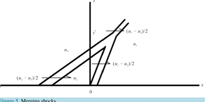
As shown in Figure 5, If ε is reasonably small, we can recognise shock transition between the states

1, 2, 3

u u u by noting in which regions the corresponding ϕ dominates. At t=0, in: 0<x, ϕ₁ dominates and we have:

( )

, 1

( )

,

( )

1 ,

u x t u x t = f ξ

2

ϕ dominates in: − < <1 x 0, then we have:

( )

, 2

( )

,

( )

2 ,

u x t u x t = f ξ

In: x< −1, ϕ₃ dominates and we obtain:

( )

, 3

( )

,

( )

3 ,

u x t u x t = f ξ

The symbol “≃” means infinitely close to [8]. Thus we have a shock transitions from u₁ to u₂ centred at 0

x= , and one from u₂ to u₃ centered at x= −1. For t>0, for early times the transition from u₁ to u₂ occurs where ϕ₁=ϕ₂ on

(

1 2

)

1

2

x= u +u t (4.14) The transition from u₂ to u₃ occurs where ϕ₂=ϕ₃ on

(

2 3

)

1

1 2

x= u +u t− (4.15)

Since, 1

(

₂ ₃

)

1

(

₁ ₂

)

2 u +u > 2 u +u , the second shock overtakes the first at the point

(

)

* *

,

x t determined by

(4.14) and (4.15). At this point

1 2 3

ϕ =ϕ =ϕ

for t>t*, there is no longer any region where ϕ₂ dominates and the continuing solution describe a single shock transition between u1 and u3, moving with the velocity

(

1 3

)

1 2

(12)

[image:12.595.147.488.89.257.2]

Figure 5. Merging shocks.

on the path determined by ϕ ϕ₁= ₃.

Acknowledgements

I thank the editor and the referee for their comments.

References

[1] Burgers, J.M. (1948) A Mathematical Model Illustrating the Theory of Turbulence. In: Von Mises, R. and Von Karman, T., Eds., Advances in Applied Mechanics, Vol. 1, Academic Press, New York, 171-199.

http://www.sciencedirect.com/science/article/pii/S0065215608701005

http://dx.doi.org/10.1016/s0065-2156(08)70100-5

[2] Burgers, J.M. (1975) The Non Linear Diffusion Equation Asymptotic Solution and Statistical Problems.

http://www.amazon.it/The-Non-Linear-Diffusion-Equation-Statistical/dp/9027704945

[3] Kida, S. (1979) Asymptotic Properties of Burgers Turbulence. Journal of Fluid Mechanics, 93, 337-377.

http://journals.cambridge.org/action/displayAbstract;jsessionid=0174C93AF976CBF18771FEB41E0FEFA9.journals?f romPage=online&aid=388434

http://dx.doi.org/10.1017/S0022112079001932

[4] Samokhin, A. (2014) Gradient Catastrophes and Saw Tooth Solution for a Generalized Burgers Equation on an Interval.

Journal of Geometry and Physics, 85, 177-184. http://www.sciencedirect.com/science/article/pii/S0393044014000965

http://dx.doi.org/10.1016/j.geomphys.2014.05.007

[5] Samokhin, A.V. (2013) Evolution of Initial Data for Burgers Equation with Fixed Boundary Values. Sci Herald of

MSTUCA, 194, 63-70. http://www.mstuca.ru/scientific_work/scientific_work/files/194.pdf

[6] Euvrard, D. (1992) Résolution Numérique des Equations aux Dérivées Partielles. Différences finies, Eléments finis. Masson, Paris.

[7] Sinai, G. (1992) Statistics of Shocks in Solutions of Inviscid Burgers Equation. Communications in Mathematical

Physics, 148, 601-621. http://citeseerx.ist.psu.edu/showciting?cid=205153

http://dx.doi.org/10.1007/bf02096550

[8] She, Z.S., Aurell, E. and Frich, U. (1992) The Inviscid Burgers Equation with Initial Data of Brownian Type. Com-

munications in Mathematical Physics, 148, 623-641.

http://www.researchgate.net/publication/38331252_The_inviscid_Burgers_equation_with_initial_data_of_Brownian_t ype

http://dx.doi.org/10.1007/BF02096551

[9] Hopf, E. (1950) The Partial Differential Equation: ut + uux= εuxx. Communications on Pure and Applied Mathematics,

3, 201-230. http://www.researchgate.net/publication/259149172_The_partial_differential_equation_ut__uux__xx

http://dx.doi.org/10.1002/cpa.3160030302

[10] Cole, J.D. (1951) On a Quasilinear Parabolic Equation Occurring in Aerodynamics. Quarterly of Applied Mathematics,

9, 225-236.

(13)

and Applied Mathematics, 41, 133-149. http://onlinelibrary.wiley.com/doi/10.1002/cpa.3160410202/abstract

http://dx.doi.org/10.1002/cpa.3160410202

[12] Kevorkian, J. and Cole, J.D. (1981) Perturbation Methods in Applied Mathematics. Springer Verlag, New York.

http://www.amazon.com/Perturbation-Methods-Mathematics-Mathematical-Sciences/dp/0387905073

http://dx.doi.org/10.1007/978-1-4757-4213-8

[13] Van Den Berg, I. (1987) Non Standard Asymptotic Analysis. Lecture Notes in Mathematics, 1249.

http://www.researchgate.net/publication/44553479_Nonstandard_asymptotic_analysis__Imme_van_den_Berg [14] Lutz, R. and Goze, M. (1981) Non Standard Analysis. A Practical Guide with Application. Lecture Notes in Mathe-

matics, 861.

[15] Lutz, R. and Sari, T. (1982) Applications of Nonstandard Analysis in Boundary Value Problems in Singular Perturbatio Theory; Theory and Application of Singular Perturbation (Oberwolfach 1981). Lecture Notes in Mathematics, 942, 113-135.

http://www.researchgate.net/publication/225547873_Applications_of_nonstandard_analysis_to_boundary_value_probl ems_in_singular_perturbation_theory

[16] Bendaas, S. (1994) Quelques applications de l’A.N.S aux E.D.P. Ph.D. Thesis, Haute Alsace University, France. [17] Bendaas, S. (2008) L’équation de Burgers avec un Terme Dissipatif. Une approche non standard. Analele Universitatii